Introduction
Feature Engineering
Figure 1
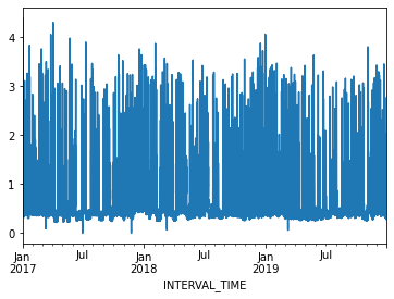
Three years’ hourly power consumption from a
single meter.
Figure 2
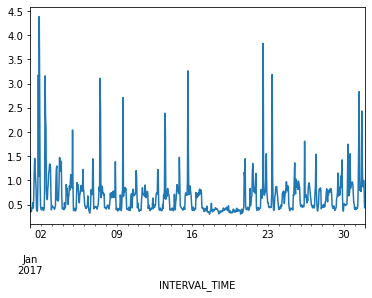
One month’s hourly power consumption from a
single meter.
Figure 3
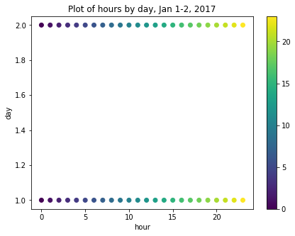
Scatter plot of days per hour, Jan 1-2,
2017.
Figure 4
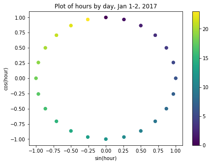
Plot of sine and cosine transformed hourly
features, Jan 1-2, 2017.
Data Windowing and Making Datasets
Figure 1
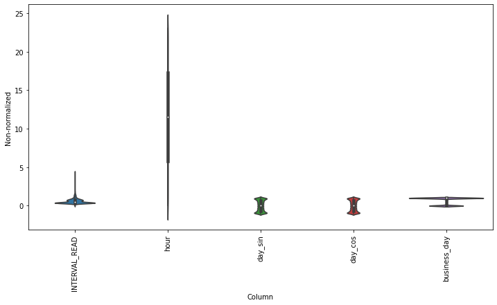
Distribution of values across features before
normalization.
Figure 2
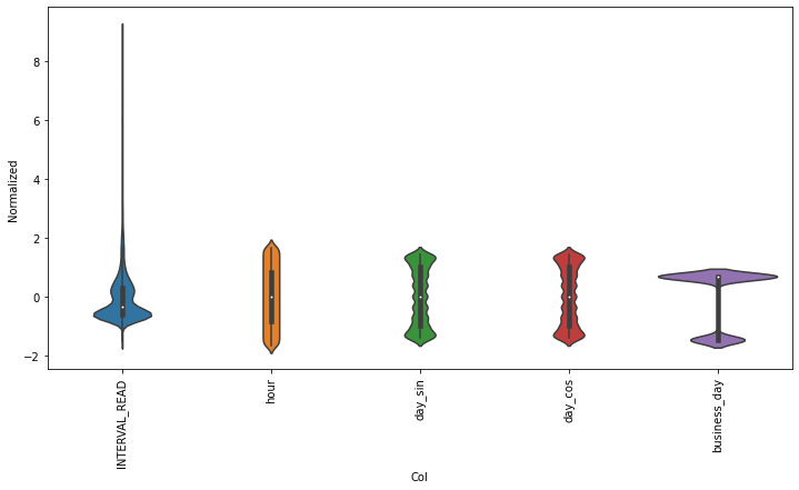
Distribution of values across features after
normalization.
Figure 3
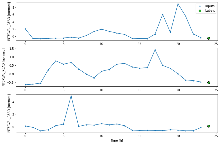
Plot of input and label values from 3 batches of
a data window.
Single Step Forecasts
Figure 1
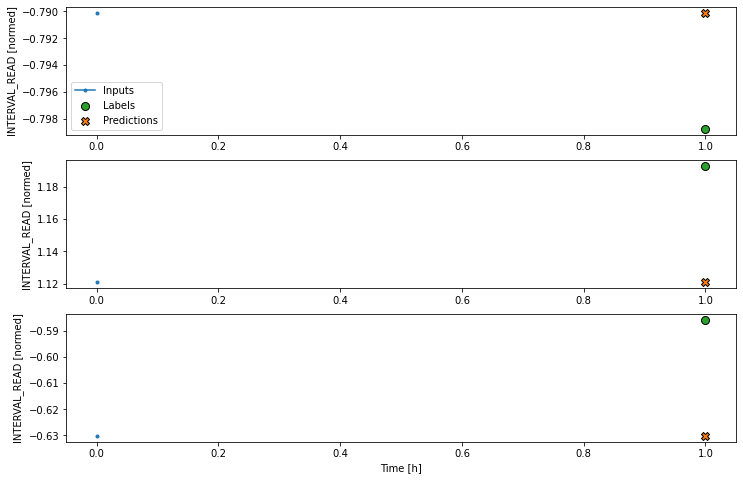
Plot of baseline forecast using a single step
window.
Figure 2
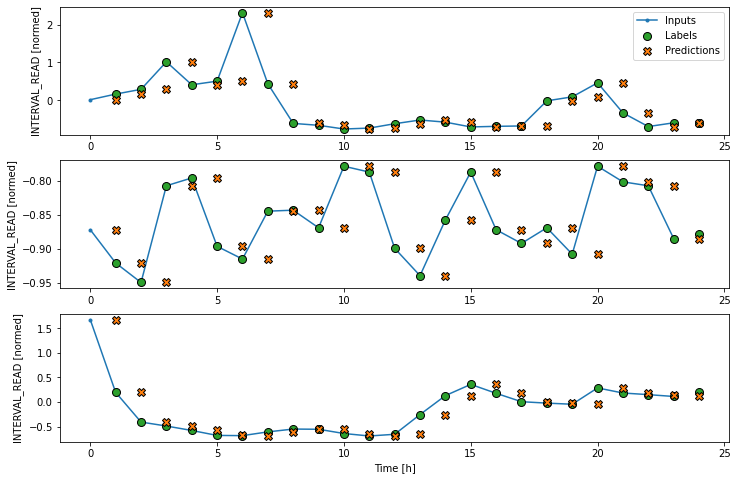
Plot of baseline forecast using a wide
window.
Figure 3
Plot of example slices of linear forecast using
a wide window.
Figure 4
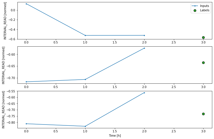
Plot of convolution window with three input and
one output timesteps.
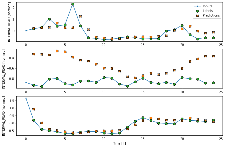
Figure 5
Plot of convolution neural network forcast using
a wide window.
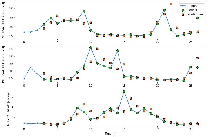
Figure 6
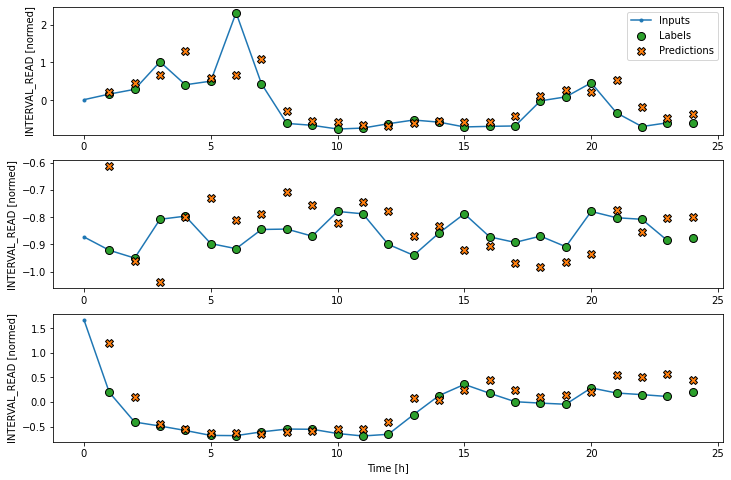
Plot of LSTM neural network forcast using a wide
window.
Figure 7
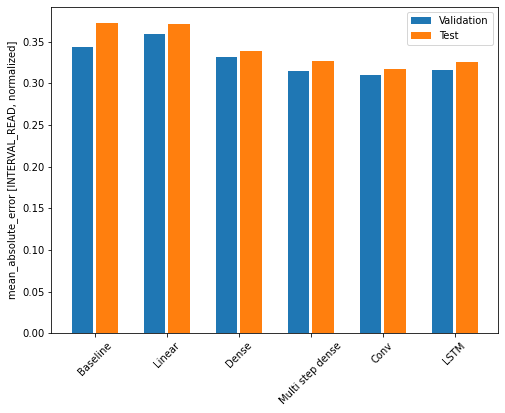
Plot comparing MAE on validation and test data
for all models.
Multi Step Forecasts
Figure 1
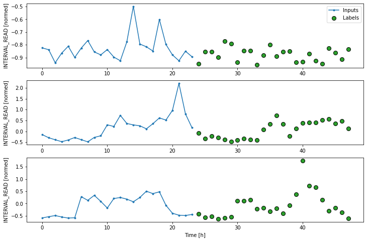
Plot of multi window input and label
widths.
Figure 2
Plot of a naive seasonal baseline model.
Figure 3
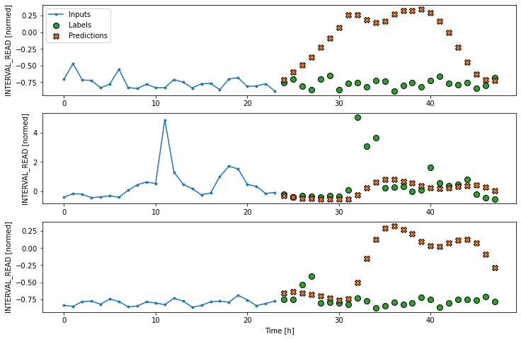
Plot of a multi step linear model.
Figure 4
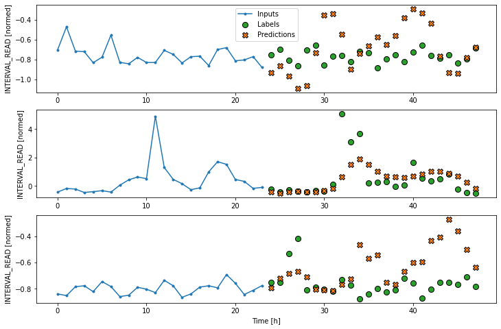
Plot of a multi step dense neural network.
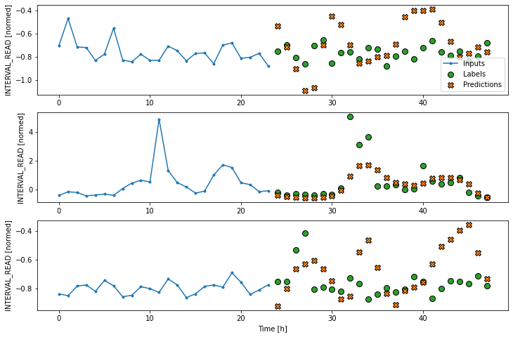
Figure 5

Plot of a multi step convolution neural
network.
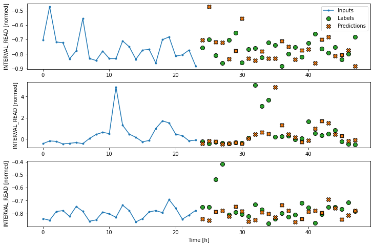
Figure 6
Plot of a multi step LSTM neural network.
Figure 7
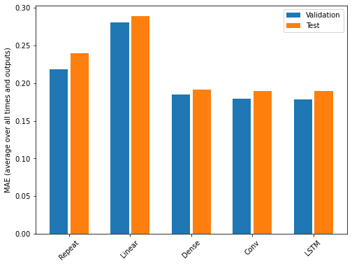
Plot of MAE of all forecasts against test and
validation data.