Single Step Forecasts
Last updated on 2023-09-01 | Edit this page
Overview
Questions
- How do we forecast one timestep in a time-series?
Objectives
- Explain how to create machine learning pipelines in
TensorFlowusing thekerasAPI.
Introduction
The previous section introduced the concept of data windows, and how they can be defined as a first step in a machine learning pipeline. Once data windows have been defined, time-series datasets can be created which consist of batches of consecutive slices of the raw data we want to model and make predictions with. Data windows not only determine the size of each slice, but also which data columns should be treated by the machine learning process as features or inputs, and which columns should be treated as labels or predicted values.
Throughout this section, we will introduce some of the time-series
modeling methods available from Google’s TensorFlow
library. We will fit and evaluate several models, each of which
demonstrates the structure of machine learning pipelines using the
keras API.
About the code
The code for this and other sections of this lesson is based on time-series forecasting examples, tutorials, and other documentation available from the TensorFlow project. Per the documentation, materials available from the TensorFlow GitHub site published using an Apache 2.0 license.
Google Inc. (2023) TensorFlow Documentation. Retrieved from https://github.com/tensorflow/docs/blob/master/README.md.
Set up the environment
In the previous section, we saved training, validation, and test
datasets that are ready to be used in our pipeline. We also wrote a
lengthy WindowGenerator class that handles the data
windowing and also creates time-series datasets out of the training,
validation, and test data.
We will reuse these files and code. For the class to load correctly, the datasets need to be read first.
Start by importing libraries.
PYTHON
import os
import IPython
import IPython.display
import matplotlib as mpl
import matplotlib.pyplot as plt
import numpy as np
import pandas as pd
import seaborn as sns
import tensorflow as tf
Now, read the training, validation, and test datasets into memory. Recall that the data were normalized in the previous section before being saved to file. They do not include all of the features of the source data, and the values have been scaled to allow more efficient processing.
PYTHON
train_df = pd.read_csv("../../data/training_df.csv")
val_df = pd.read_csv("../../data/val_df.csv")
test_df = pd.read_csv("../../data/test_df.csv")

column_indices = {name: i for i, name in enumerate(test_df.columns)}

print(train_df.info())
print(val_df.info())
print(test_df.info())
print(column_indices)
OUTPUT
<class 'pandas.core.frame.DataFrame'>
RangeIndex: 18396 entries, 0 to 18395
Data columns (total 5 columns):
 #   Column         Non-Null Count  Dtype
---  ------         --------------  -----
 0   INTERVAL_READ  18396 non-null  float64
 1   hour           18396 non-null  float64
 2   day_sin        18396 non-null  float64
 3   day_cos        18396 non-null  float64
 4   business_day   18396 non-null  float64
dtypes: float64(5)
memory usage: 718.7 KB
None

<class 'pandas.core.frame.DataFrame'>
RangeIndex: 5256 entries, 0 to 5255
Data columns (total 5 columns):
 #   Column         Non-Null Count  Dtype
---  ------         --------------  -----
 0   INTERVAL_READ  5256 non-null   float64
 1   hour           5256 non-null   float64
 2   day_sin        5256 non-null   float64
 3   day_cos        5256 non-null   float64
 4   business_day   5256 non-null   float64
dtypes: float64(5)
memory usage: 205.4 KB
None

<class 'pandas.core.frame.DataFrame'>
RangeIndex: 2628 entries, 0 to 2627
Data columns (total 5 columns):
 #   Column         Non-Null Count  Dtype
---  ------         --------------  -----
 0   INTERVAL_READ  2628 non-null   float64
 1   hour           2628 non-null   float64
 2   day_sin        2628 non-null   float64
 3   day_cos        2628 non-null   float64
 4   business_day   2628 non-null   float64
dtypes: float64(5)
memory usage: 102.8 KB
None

{'INTERVAL_READ': 0, 'hour': 1, 'day_sin': 2, 'day_cos': 3, 'business_day': 4}
With our data loaded, we can now define the
WindowGenerator class. Note that this is all the same code
as we previously developed. Whereas earlier we developed the code in
sections and walked through a description of what each function does,
here we are simply copying all of the class code in at once.
PYTHON
class WindowGenerator():
  def __init__(self, input_width, label_width, shift,
               train_df=train_df, val_df=val_df, test_df=test_df,
               label_columns=None):
    # Store the raw data.
    self.train_df = train_df
    self.val_df = val_df
    self.test_df = test_df

    # Work out the label column indices.
    self.label_columns = label_columns
    if label_columns is not None:
      self.label_columns_indices = {name: i for i, name in
                                    enumerate(label_columns)}
    self.column_indices = {name: i for i, name in
                           enumerate(train_df.columns)}

    # Work out the window parameters.
    self.input_width = input_width
    self.label_width = label_width
    self.shift = shift

    self.total_window_size = input_width + shift

    self.input_slice = slice(0, input_width)
    self.input_indices = np.arange(self.total_window_size)[self.input_slice]

    self.label_start = self.total_window_size - self.label_width
    self.labels_slice = slice(self.label_start, None)
    self.label_indices = np.arange(self.total_window_size)[self.labels_slice]


  def __repr__(self):
    return '\n'.join([
        f'Total window size: {self.total_window_size}',
        f'Input indices: {self.input_indices}',
        f'Label indices: {self.label_indices}',
        f'Label column name(s): {self.label_columns}'])


  def split_window(self, features):
    inputs = features[:, self.input_slice, :]
    labels = features[:, self.labels_slice, :]
    if self.label_columns is not None:
      labels = tf.stack(
          [labels[:, :, self.column_indices[name]] for name in self.label_columns],
          axis=-1)

    # Slicing doesn't preserve static shape information, so set the shapes
    # manually. This way the `tf.data.Datasets` are easier to inspect.
    inputs.set_shape([None, self.input_width, None])
    labels.set_shape([None, self.label_width, None])

    return inputs, labels


  def plot(self, model=None, plot_col='INTERVAL_READ', max_subplots=3):
    inputs, labels = self.example
    plt.figure(figsize=(12, 8))
    plot_col_index = self.column_indices[plot_col]
    max_n = min(max_subplots, len(inputs))
    for n in range(max_n):
      plt.subplot(max_n, 1, n+1)
      plt.ylabel(f'{plot_col} [normed]')
      plt.plot(self.input_indices, inputs[n, :, plot_col_index],
               label='Inputs', marker='.', zorder=-10)

      if self.label_columns:
        label_col_index = self.label_columns_indices.get(plot_col, None)
      else:
        label_col_index = plot_col_index

      if label_col_index is None:
        continue

      plt.scatter(self.label_indices, labels[n, :, label_col_index],
                  edgecolors='k', label='Labels', c='#2ca02c', s=64)
      if model is not None:
        predictions = model(inputs)
        plt.scatter(self.label_indices, predictions[n, :, label_col_index],
                    marker='X', edgecolors='k', label='Predictions',
                    c='#ff7f0e', s=64)

      if n == 0:
        plt.legend()

    plt.xlabel('Time [h]')


  def make_dataset(self, data):
    data = np.array(data, dtype=np.float32)
    ds = tf.keras.utils.timeseries_dataset_from_array(
        data=data,
        targets=None,
        sequence_length=self.total_window_size,
        sequence_stride=1,
        shuffle=True,
        batch_size=32)

    ds = ds.map(self.split_window)

    return ds


  @property
  def train(self):
    return self.make_dataset(self.train_df)

  @property
  def val(self):
    return self.make_dataset(self.val_df)

  @property
  def test(self):
    return self.make_dataset(self.test_df)

  @property
  def example(self):
    """Get and cache an example batch of `inputs, labels` for plotting."""
    result = getattr(self, '_example', None)
    if result is None:
      # No example batch was found, so get one from the `.train` dataset
      result = next(iter(self.train))
      # And cache it for next time
      self._example = result
    return result
It is recommended to execute the script or code block that contains the class definition before proceeding, to make sure there are no spacing or syntax errors.
Callout
Copying and pasting is generally discouraged, so an alternative to
copying and pasting the class definition above is to save the class to a
file and import it using from WindowGenerator import *.
This will be added to an update of this lesson, but note in the meantime
that the dataframes for train_df, val_df, and test_df are dependencies.
Importing the class definition as a standalone script at this time
requires those to be included in the definition as keyword arguments
that are explicitly defined when a WindowGenerator object
is instantiated.
Create data windows
For our initial pass at single-step forecasting, we are going to define a data window that we will use to make a single forecast (label_width), one hour into the future (shift), based on one hour of history (input_width). The column that we are making predictions for is INTERVAL_READ.
PYTHON
# forecast one step at a time based on previous step

# single prediction (label width), 1 hour into future (shift)
# with 1h history (input width)
# forecasting "INTERVAL_READ"

single_step_window = WindowGenerator(
    input_width=1, label_width=1, shift=1,
    label_columns=['INTERVAL_READ'])

print(single_step_window)
OUTPUT
Total window size: 2
Input indices: [0]
Label indices: [1]
Label column name(s): ['INTERVAL_READ']
We can inspect the resulting training time-series data to confirm that it has been split into 575 batches of 32 arrays or slices (except for the last batch, which may be smaller), with each slice containing an input shape of 1 timestep and 5 features and a label shape of 1 timestep and 1 feature.
PYTHON
print("Number of batches:", len(single_step_window.train))

for example_inputs, example_labels in single_step_window.train.take(1):
  print(f'Inputs shape (batch, time, features): {example_inputs.shape}')
  print(f'Labels shape (batch, time, features): {example_labels.shape}')
OUTPUT
Number of batches: 575
Inputs shape (batch, time, features): (32, 1, 5)
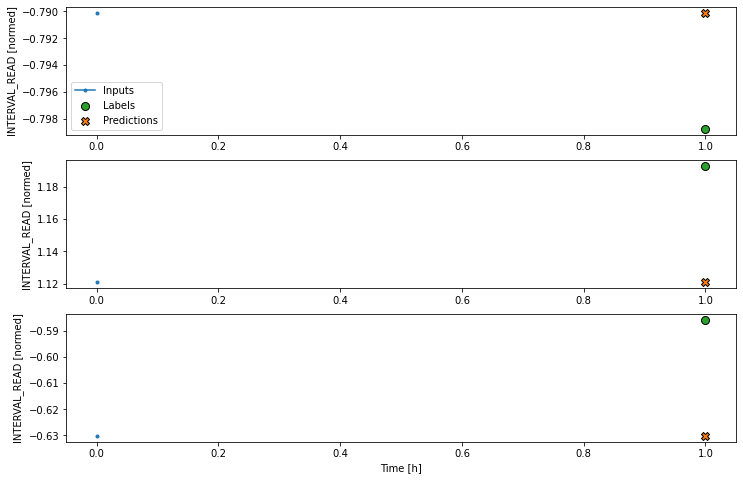
Labels shape (batch, time, features): (32, 1, 1)We will see below that a single step window doesn’t produce a very
informative plot, due to its total window size of 2 timesteps. For
plotting purposes, we will also define a wide window. Note that this
does not impact the forecasts, as the way in which the
WindowGenerator class has been defined allows us to fit a
model using the single step window and plot the forecasts from that same
model using the wide window.
PYTHON
wide_window = WindowGenerator(
    input_width=24, label_width=24, shift=1,
    label_columns=['INTERVAL_READ'])

print(wide_window)
OUTPUT
Total window size: 25
Input indices: [ 0  1  2  3  4  5  6  7  8  9 10 11 12 13 14 15 16 17 18 19 20 21 22 23]
Label indices: [ 1  2  3  4  5  6  7  8  9 10 11 12 13 14 15 16 17 18 19 20 21 22 23 24]
Label column name(s): ['INTERVAL_READ']
Define basline forecast
As with any modeling process, it is important to establish a baseline
forecast against which to compare and evaluate each model’s performance.
In this case, we will continue to use the last known value as the
baseline forecast, only this time we define the model as a subclass of a
TensorFlow model. This allows the model to access
TensorFlow methods and attributes.
PYTHON
class Baseline(tf.keras.Model):
  def __init__(self, label_index=None):
    super().__init__()
    self.label_index = label_index

  def call(self, inputs):
    if self.label_index is None:
      return inputs
    result = inputs[:, :, self.label_index]
    return result[:, :, tf.newaxis]
Next, we create an instance of the Baseline class and
configure it for training using the compile() method. We
pass two arguments - the loss function, which measures the difference
between predicted and actual values. In this case, as in the other
models we will define below, the loss function is the mean squared
error. As the model is trained and fit, the loss function is used to
assess when predictions cease to improve significantly in proportion to
the cost of continuing to train the model further.
The second argument is the metric against which the overall performance of the model is evaluated. The metric in this case, and in other models below, is the mean absolute error.
After creating some empty dictionaries to store performance metrics,
the model is evaluated using the evalute() method to return
the mean squared error (loss value) and performance metric (mean
absolute error) of the model against the validation and test
dataframes.
PYTHON
baseline = Baseline(label_index=column_indices['INTERVAL_READ'])

baseline.compile(loss=tf.keras.losses.MeanSquaredError(),
                 metrics=[tf.keras.metrics.MeanAbsoluteError()])

val_performance = {}
performance = {}

val_performance['Baseline'] = baseline.evaluate(single_step_window.val)
performance['Baseline'] = baseline.evaluate(single_step_window.test, verbose=0)

print("Basline performance against validation data:", val_performance["Baseline"])
print("Basline performance against test data:", performance["Baseline"])
OUTPUT
165/165 [==============================] - 0s 2ms/step - loss: 0.5926 - mean_absolute_error: 0.3439

Basline performance against validation data: [0.5925938487052917, 0.34389233589172363]
Basline performance against test data: [0.6656807661056519, 0.37295007705688477]
Note that when the model is evaluated a progress bar is provided that shows how many batches have been evaluated so far, as long as the amount of time taken per batch. In our example, the number 165 comes from the total length of the validation dataframe (5256) divided by the number of slices within each batch (32):
OUTPUT
164.25Given that the number of slices in a batch can only be a whole number, we can assume that the last two batches included less than 32 slices apiece.
The loss and mean_absolute_error metrics are those specified when we compiled the model, above.
We can try to plot the inputs, labels, and predictions of an example set of three slices of the data using the single step window. As noted above, however, the plot is not informative. The single input appears on the left, with the predicted next timestep and the forecast next timestep all the way to the right. The entire plot only covers two timesteps.
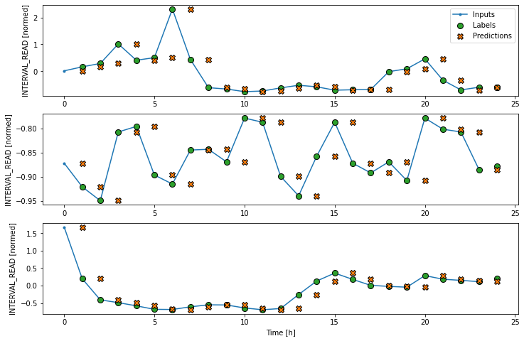
Instead, we can plot the model’s predictions using the wide window. Note that the model is not being re-evaluated. We are instead using the wide window to request and plot a larger number of predictions.
We are now ready to train models. With the addition of creating
layered neural networks using the keras API, all of the
models below will be fitted and evaluated using a workflow similar to
that which we used for the baseline model, above. Rather than repeat the
same code multiple times, before we go any further we will write a
function to encapsulate the process.
The function adds some features to the workflow. As noted above, the loss function acts as a measure of the trade-off between computational costs and accuracy. As the model is fitted, the loss function is used to monitor the model’s efficiency and provides the model an internal mechanism for determining a stopping point.
The compile() method is similar to the above, with the
addition of an optimizer argument. The optimizer is an
algorithm that determines the most efficient weights for each feature as
the model is fitted. In the current example, we are using the
Adam() optimizer that is included as part of the default
TensorFlow library.
Finally, the model is fit using the training dataframe. The data are split using the data window specified in the positional window argument, in our case the single step window defined above. Predictions are validated against the validation data, with the process configured to halt at the point that accuracy no longer improves.
The epochs argument represented the number of times the that the model will work through the entire training dataframe, provided it is not stopped before it reaches that number by the loss function. Note that the MAX_EPOCHS is being manually set in the code block below.
PYTHON
MAX_EPOCHS = 20

def compile_and_fit(model, window, patience=2):
  early_stopping = tf.keras.callbacks.EarlyStopping(monitor='val_loss',
                                                    patience=patience,
                                                    mode='min')

  model.compile(loss=tf.keras.losses.MeanSquaredError(),
                optimizer=tf.keras.optimizers.Adam(),
                metrics=[tf.keras.metrics.MeanAbsoluteError()])

  history = model.fit(window.train, epochs=MAX_EPOCHS,
                      validation_data=window.val,
                      callbacks=[early_stopping])
  return history
Linear model
keras in an API that provides access to
TensorFlow machine learning methods and utilities.
Throughout the remained of this and other sections of this lesson, we
will the API to define classes of neural networks using the API’s
layers class. In particular, we will develop workflows that
use linear stacks of layers to build models using the
Sequential subclass of tf.keras.Model.
The first model we will create is a linear model, which is the
default for a Dense layer for which an activation function
is not defined. We will see examples of activation functions below.
PYTHON
linear = tf.keras.Sequential([
    tf.keras.layers.Dense(units=1)
])

print('Input shape:', single_step_window.example[0].shape)
print('Output shape:', linear(single_step_window.example[0]).shape)
OUTPUT
Input shape: (32, 1, 5)
Output shape: (32, 1, 1)
Recall that we are using the single step window to fit and evaluate our models. The output above confirms that the data have been split into input batches of 32 slices. Each input slice consists of a single timestep and five features. The output of the model is likewise split into 32 batches, where each batch consists of 1 timestep and one feature (the forecast value of INTERVAL_READ).
We compile, fit, and evaluate the model using the
compile_and_fit() function above.
PYTHON
history = compile_and_fit(linear, single_step_window)

val_performance['Linear'] = linear.evaluate(single_step_window.val)
performance['Linear'] = linear.evaluate(single_step_window.test, verbose=0)

print("Linear performance against validation data:", val_performance["Linear"])
print("Linear performance against test data:", performance["Linear"])
The output is long, and may vary between executions. In the case below, we can see that the model was fitted against the entire training dataframe ten times before stopping as determined by the loss function. After the final run, the performance was measure against the validation dataframe, and the mean absolute error of the predicted INTERVAL_READ values against the actual values in the validation and test dataframes are requested. These are added to the val_performance and performance dictionaries created above.
OUTPUT
Epoch 1/20
575/575 [==============================] - 1s 2ms/step - loss: 3.8012 - mean_absolute_error: 1.4399 - val_loss: 2.1368 - val_mean_absolute_error: 1.1136
Epoch 2/20
575/575 [==============================] - 1s 941us/step - loss: 1.8124 - mean_absolute_error: 0.9400 - val_loss: 1.0215 - val_mean_absolute_error: 0.7250
Epoch 3/20
575/575 [==============================] - 1s 949us/step - loss: 0.9970 - mean_absolute_error: 0.6313 - val_loss: 0.6207 - val_mean_absolute_error: 0.5071
Epoch 4/20
575/575 [==============================] - 1s 949us/step - loss: 0.7053 - mean_absolute_error: 0.4852 - val_loss: 0.5003 - val_mean_absolute_error: 0.4196
Epoch 5/20
575/575 [==============================] - 1s 993us/step - loss: 0.6123 - mean_absolute_error: 0.4306 - val_loss: 0.4674 - val_mean_absolute_error: 0.3835
Epoch 6/20
575/575 [==============================] - 1s 1ms/step - loss: 0.5851 - mean_absolute_error: 0.4075 - val_loss: 0.4597 - val_mean_absolute_error: 0.3686
Epoch 7/20
575/575 [==============================] - 1s 967us/step - loss: 0.5784 - mean_absolute_error: 0.3978 - val_loss: 0.4584 - val_mean_absolute_error: 0.3622
Epoch 8/20
575/575 [==============================] - 1s 967us/step - loss: 0.5772 - mean_absolute_error: 0.3943 - val_loss: 0.4583 - val_mean_absolute_error: 0.3599
Epoch 9/20
575/575 [==============================] - 1s 949us/step - loss: 0.5770 - mean_absolute_error: 0.3931 - val_loss: 0.4585 - val_mean_absolute_error: 0.3598
Epoch 10/20
575/575 [==============================] - 1s 958us/step - loss: 0.5770 - mean_absolute_error: 0.3927 - val_loss: 0.4586 - val_mean_absolute_error: 0.3592
165/165 [==============================] - 0s 732us/step - loss: 0.4586 - mean_absolute_error: 0.3592
Linear performance against validation data: [0.45858854055404663, 0.3591674864292145]
Linear performance against test data: [0.5238229036331177, 0.3708552420139313]
For additional models, the output provided here will only consist of the final epoch’s progress and the performance metrics.
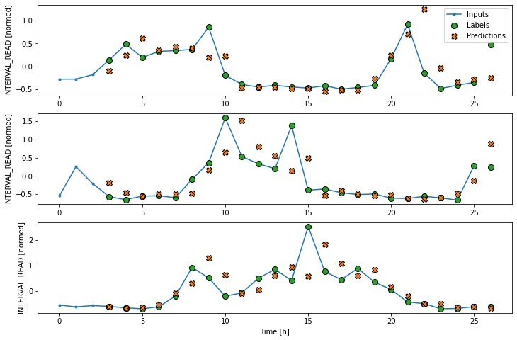
As above, although the model was fitted using the single step window, we can generate a more interesting plot using the wide window. Recall that we are not plotting the entire dataset here, but only three example slices of 25 timesteps each.
Dense neural network
We can build more complex models by adding layers to the stack. The
following defines a dense neural network that consists of three layers.
All three are Dense layers, but the first two use an
relu activation function.
PYTHON
dense = tf.keras.Sequential([
    tf.keras.layers.Dense(units=64, activation='relu'),
    tf.keras.layers.Dense(units=64, activation='relu'),
    tf.keras.layers.Dense(units=1)
])

# Run the model as above
history = compile_and_fit(dense, single_step_window)

val_performance['Dense'] = dense.evaluate(single_step_window.val)
performance['Dense'] = dense.evaluate(single_step_window.test, verbose=0)

print("DNN performance against validation data:", val_performance["Dense"])
print("DNN performance against test data:", performance["Dense"])
OUTPUT
Epoch 9/20
575/575 [==============================] - 1s 2ms/step - loss: 0.4793 - mean_absolute_error: 0.3420 - val_loss: 0.4020 - val_mean_absolute_error: 0.3312
165/165 [==============================] - 0s 1ms/step - loss: 0.4020 - mean_absolute_error: 0.3312
DNN performance against validation data: [0.40203145146369934, 0.3312338590621948]
DNN performance against test data: [0.43506449460983276, 0.33891454339027405]
So far we have been using a single timestep to predict the INTERVAL_READ value of the next timestep. The accuracy of models based on a single step window is limited, because many time-based measurements like power consumption can exhibit autoregressive processes. The models that we have trained so far are single step models, in the sense that they are not structured to handle multiple inputs in order to predict a single output.
Adding new processing layers to the model stacks we’re defining allows us to handle longer input values or timesteps in order to forecast a single output label or timestep. We will start by revising the dense neural network above to flatten and reshape multiple inputs, but first we will define a new data window. This data window will predict one hour of power consumption (label_width), one hour in the future (shift), using three hours of history (input_width.)
PYTHON
CONV_WIDTH = 3
conv_window = WindowGenerator(
    input_width=CONV_WIDTH,
    label_width=1,
    shift=1,
    label_columns=['INTERVAL_READ'])

print(conv_window)
OUTPUT
Total window size: 4
Input indices: [0 1 2]
Label indices: [3]
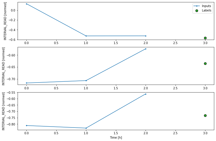
Label column name(s): ['INTERVAL_READ']If we plot the conv_window example slices, we see that
although not as wide as the wide window we have been using to plot
forecasts, in contrast with the single step window this plot includes
three input timesteps and one label timestep. Recall that the label is
the actual value that a forecast is measured against.
Now we can modify the above dense model to flatten and reshape the data to account for the multiple inputs.
PYTHON
multi_step_dense = tf.keras.Sequential([
    tf.keras.layers.Flatten(),
    tf.keras.layers.Dense(units=32, activation='relu'),
    tf.keras.layers.Dense(units=32, activation='relu'),
    tf.keras.layers.Dense(units=1),
    tf.keras.layers.Reshape([1, -1]),
])

history = compile_and_fit(multi_step_dense, conv_window)

val_performance['Multi step dense'] = multi_step_dense.evaluate(conv_window.val)
performance['Multi step dense'] = multi_step_dense.evaluate(conv_window.test, verbose=0)

print("MSD performance against validation data:", val_performance["Multi step dense"])
print("MSD performance against test data:", performance["Multi step dense"])
OUTPUT
Epoch 10/20
575/575 [==============================] - 1s 2ms/step - loss: 0.4693 - mean_absolute_error: 0.3421 - val_loss: 0.3829 - val_mean_absolute_error: 0.3080
165/165 [==============================] - 0s 1ms/step - loss: 0.3829 - mean_absolute_error: 0.3080
MSD performance against validation data: [0.3829467296600342, 0.30797266960144043]
MSD performance against test data: [0.4129006564617157, 0.3209587633609772]
We can see from the performance metrics that our models are gradually improving.
Convolution neural network
A convolution neural network is similar to the multi-step dense model we defined above, with the difference that a convolution layer can accept multiple timesteps as input without requiring additional layers to flatten and reshape the data.
PYTHON
conv_model = tf.keras.Sequential([
    tf.keras.layers.Conv1D(filters=32,
                           kernel_size=(CONV_WIDTH,),
                           activation='relu'),
    tf.keras.layers.Dense(units=32, activation='relu'),
    tf.keras.layers.Dense(units=1),
])


history = compile_and_fit(conv_model, conv_window)

val_performance['Conv'] = conv_model.evaluate(conv_window.val)
performance['Conv'] = conv_model.evaluate(conv_window.test, verbose=0)

print("CNN performance against validation data:", val_performance["Conv"])
print("CNN performance against test data:", performance["Conv"])
Epoch 7/20
575/575 [==============================] - 1s 2ms/step - loss: 0.4744 - mean_absolute_error: 0.3414 - val_loss: 0.3887 - val_mean_absolute_error: 0.3100
165/165 [==============================] - 0s 1ms/step - loss: 0.3887 - mean_absolute_error: 0.3100
CNN performance against validation data: [0.38868486881256104, 0.3099767565727234]
CNN performance against test data: [0.41420620679855347, 0.31745821237564087]In order to plot the results, we need to define a new wide window for convolution models.
PYTHON
LABEL_WIDTH = 24
INPUT_WIDTH = LABEL_WIDTH + (CONV_WIDTH - 1)
wide_conv_window = WindowGenerator(
    input_width=INPUT_WIDTH,
    label_width=LABEL_WIDTH,
    shift=1,
    label_columns=['INTERVAL_READ'])

print(wide_conv_window)
OUTPUT
Total window size: 27
Input indices: [ 0 1 2 3 4 5 6 7 8 9 10 11 12 13 14 15 16 17 18 19 20 21 22 23
24 25]
Label indices: [ 3 4 5 6 7 8 9 10 11 12 13 14 15 16 17 18 19 20 21 22 23 24 25 26]
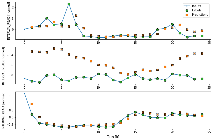
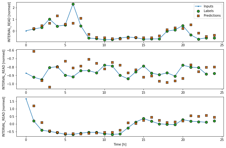
Label column name(s): ['INTERVAL_READ']Now we can plot the result.
Recurrent neural network
Alternatively, a recurrent neural network is a model that processes time-series in single steps but maintains an internal state that is updated on a step by step basis. A recurrent neural network layer that is commonly used for time-series analysis is called Long Short-Term Memory or LSTM.
Note that in the process below, we return to using our wide window as the single step data window.
PYTHON
lstm_model = tf.keras.models.Sequential([
    tf.keras.layers.LSTM(32, return_sequences=True),
    tf.keras.layers.Dense(units=1)
])

history = compile_and_fit(lstm_model, wide_window)

val_performance['LSTM'] = lstm_model.evaluate(wide_window.val)
performance['LSTM'] = lstm_model.evaluate(wide_window.test, verbose=0)


print("LSTM performance against validation data:", val_performance["LSTM"])
print("LSTM performance against test data:", performance["LSTM"])
OUTPUT
Epoch 4/20
575/575 [==============================] - 4s 7ms/step - loss: 0.4483 - mean_absolute_error: 0.3307 - val_loss: 0.3776 - val_mean_absolute_error: 0.3162
164/164 [==============================] - 0s 3ms/step - loss: 0.3776 - mean_absolute_error: 0.3162
LSTM performance against validation data: [0.3776029646396637, 0.3161604404449463]
LSTM performance against test data: [0.4038854241371155, 0.3253307044506073]
Plot the result.
Evalute the models
Recall that we are using the mean absolute error as the performance metric for evaluating predictions against actual values in the test dataframe. Since we have been storing these values in a dictionary, we can compare the performance of each model by looping through the dictionary.
OUTPUT
Baseline    : 0.3730
Linear      : 0.3709
Dense       : 0.3389
Multi step dense: 0.3272
Conv        : 0.3175
LSTM        : 0.3253
Note that results may vary. In the development of this lesson, the best performing model alternated between the convolution neural network and the LSTM.
The output above provides a comparison of mean absolute error for all models agains the test dataframe. We can also compare their respective performance by plotting the mean absolute error of each model against both the validation and test dataframes.
PYTHON
x = np.arange(len(performance))
width = 0.3
metric_name = 'mean_absolute_error'
metric_index = lstm_model.metrics_names.index('mean_absolute_error')
val_mae = [v[metric_index] for v in val_performance.values()]
test_mae = [v[metric_index] for v in performance.values()]

plt.ylabel('mean_absolute_error [INTERVAL_READ, normalized]')
plt.bar(x - 0.17, val_mae, width, label='Validation')
plt.bar(x + 0.17, test_mae, width, label='Test')
plt.xticks(ticks=x, labels=performance.keys(),
           rotation=45)
_ = plt.legend()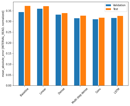
Key Points
- Use the
kerasAPI to define neural network layers and attributes to construct different machine learning pipelines.