Multi Step Forecasts
Last updated on 2023-08-31 | Edit this page
Overview
Questions
- How can forecast more than one timestep at a time?
Objectives
- Explain how to create data windows and machine learning pipelines for forcasting multiple timesteps.
Introduction
In the previous section we developed models for making forecasts one timestep into the future. Our data consist of hourly totals of power consumption from a single smart meter, and most of the models were fitted using a one hour input width to predict the next hour’s power consumption. Recall that the best performing model, the convolution neural network, differed in that the model was fitted using a data window with a three hour input width. This implies that, at least for our data, data windows with larger input widths may increase the predictive power of the models.
In this section we will revisit the same models as before, only this time we will revise our data windows to predict multiple timesteps. Specifically, we will forecast a full day’s worth of hourly power consumption based on the previous day’s history. In terms of data window arguments, both the input_width and the label_width will be equal to 24.
About the code
The code for this and other sections of this lesson is based on time-series forecasting examples, tutorials, and other documentation available from the TensorFlow project. Per the documentation, materials available from the TensorFlow GitHub site published using an Apache 2.0 license.
Google Inc. (2023) TensorFlow Documentation. Retrieved from https://github.com/tensorflow/docs/blob/master/README.md.
Set up the environment
As with the previous section, begin by importing libraries, reading
data, and defining the WindowGenerator class.
PYTHON
import os
import IPython
import IPython.display
import matplotlib as mpl
import matplotlib.pyplot as plt
import numpy as np
import pandas as pd
import seaborn as sns
import tensorflow as tf
Read the data. These are the normalized training, validation, and test datasets we created in the data windowing episode. In addition to being normalized, columns with non-numeric data types have been removed from the source data. Also, based on multiple iterations of the modeling process some additional, numeric columns were dropped.
PYTHON
train_df = pd.read_csv("../../data/training_df.csv")
val_df = pd.read_csv("../../data/val_df.csv")
test_df = pd.read_csv("../../data/test_df.csv")

column_indices = {name: i for i, name in enumerate(test_df.columns)}

print(train_df.info())
print(val_df.info())
print(test_df.info())
print(column_indices)
OUTPUT
<class 'pandas.core.frame.DataFrame'>
RangeIndex: 18396 entries, 0 to 18395
Data columns (total 5 columns):
 #   Column         Non-Null Count  Dtype
---  ------         --------------  -----
 0   INTERVAL_READ  18396 non-null  float64
 1   hour           18396 non-null  float64
 2   day_sin        18396 non-null  float64
 3   day_cos        18396 non-null  float64
 4   business_day   18396 non-null  float64
dtypes: float64(5)
memory usage: 718.7 KB
None

<class 'pandas.core.frame.DataFrame'>
RangeIndex: 5256 entries, 0 to 5255
Data columns (total 5 columns):
 #   Column         Non-Null Count  Dtype
---  ------         --------------  -----
 0   INTERVAL_READ  5256 non-null   float64
 1   hour           5256 non-null   float64
 2   day_sin        5256 non-null   float64
 3   day_cos        5256 non-null   float64
 4   business_day   5256 non-null   float64
dtypes: float64(5)
memory usage: 205.4 KB
None

<class 'pandas.core.frame.DataFrame'>
RangeIndex: 2628 entries, 0 to 2627
Data columns (total 5 columns):
 #   Column         Non-Null Count  Dtype
---  ------         --------------  -----
 0   INTERVAL_READ  2628 non-null   float64
 1   hour           2628 non-null   float64
 2   day_sin        2628 non-null   float64
 3   day_cos        2628 non-null   float64
 4   business_day   2628 non-null   float64
dtypes: float64(5)
memory usage: 102.8 KB
None

{'INTERVAL_READ': 0, 'hour': 1, 'day_sin': 2, 'day_cos': 3, 'business_day': 4}
Finally, create the WindowGenerator class.
PYTHON
class WindowGenerator():
  def __init__(self, input_width, label_width, shift,
               train_df=train_df, val_df=val_df, test_df=test_df,
               label_columns=None):
    # Store the raw data.
    self.train_df = train_df
    self.val_df = val_df
    self.test_df = test_df

    # Work out the label column indices.
    self.label_columns = label_columns
    if label_columns is not None:
      self.label_columns_indices = {name: i for i, name in
                                    enumerate(label_columns)}
    self.column_indices = {name: i for i, name in
                           enumerate(train_df.columns)}

    # Work out the window parameters.
    self.input_width = input_width
    self.label_width = label_width
    self.shift = shift

    self.total_window_size = input_width + shift

    self.input_slice = slice(0, input_width)
    self.input_indices = np.arange(self.total_window_size)[self.input_slice]

    self.label_start = self.total_window_size - self.label_width
    self.labels_slice = slice(self.label_start, None)
    self.label_indices = np.arange(self.total_window_size)[self.labels_slice]


  def __repr__(self):
    return '\n'.join([
        f'Total window size: {self.total_window_size}',
        f'Input indices: {self.input_indices}',
        f'Label indices: {self.label_indices}',
        f'Label column name(s): {self.label_columns}'])


  def split_window(self, features):
    inputs = features[:, self.input_slice, :]
    labels = features[:, self.labels_slice, :]
    if self.label_columns is not None:
      labels = tf.stack(
          [labels[:, :, self.column_indices[name]] for name in self.label_columns],
          axis=-1)

    # Slicing doesn't preserve static shape information, so set the shapes
    # manually. This way the `tf.data.Datasets` are easier to inspect.
    inputs.set_shape([None, self.input_width, None])
    labels.set_shape([None, self.label_width, None])

    return inputs, labels


  def plot(self, model=None, plot_col='INTERVAL_READ', max_subplots=3):
    inputs, labels = self.example
    plt.figure(figsize=(12, 8))
    plot_col_index = self.column_indices[plot_col]
    max_n = min(max_subplots, len(inputs))
    for n in range(max_n):
      plt.subplot(max_n, 1, n+1)
      plt.ylabel(f'{plot_col} [normed]')
      plt.plot(self.input_indices, inputs[n, :, plot_col_index],
               label='Inputs', marker='.', zorder=-10)

      if self.label_columns:
        label_col_index = self.label_columns_indices.get(plot_col, None)
      else:
        label_col_index = plot_col_index

      if label_col_index is None:
        continue

      plt.scatter(self.label_indices, labels[n, :, label_col_index],
                  edgecolors='k', label='Labels', c='#2ca02c', s=64)
      if model is not None:
        predictions = model(inputs)
        plt.scatter(self.label_indices, predictions[n, :, label_col_index],
                    marker='X', edgecolors='k', label='Predictions',
                    c='#ff7f0e', s=64)

      if n == 0:
        plt.legend()

    plt.xlabel('Time [h]')


  def make_dataset(self, data):
    data = np.array(data, dtype=np.float32)
    ds = tf.keras.utils.timeseries_dataset_from_array(
        data=data,
        targets=None,
        sequence_length=self.total_window_size,
        sequence_stride=1,
        shuffle=True,
        batch_size=32)

    ds = ds.map(self.split_window)

    return ds


  @property
  def train(self):
    return self.make_dataset(self.train_df)

  @property
  def val(self):
    return self.make_dataset(self.val_df)

  @property
  def test(self):
    return self.make_dataset(self.test_df)

  @property
  def example(self):
    """Get and cache an example batch of `inputs, labels` for plotting."""
    result = getattr(self, '_example', None)
    if result is None:
      # No example batch was found, so get one from the `.train` dataset
      result = next(iter(self.train))
      # And cache it for next time
      self._example = result
    return result
Create a multi-step data window
Create a data window that will forecast 24 timesteps (label_width), 24 hours into the future (shift), based on 24 hours of history (input_width).
Since the value of the label_width and shift arguments are used to set model parameters later, we will stored this value in a variable. This way, if we want to test different label widths and shift values we only need to update the OUT_STEPS variable.
PYTHON
OUT_STEPS = 24
multi_window = WindowGenerator(input_width=24,
                               label_width=OUT_STEPS,
                               shift=OUT_STEPS)

print(multi_window)
OUTPUT
Total window size: 48
Input indices: [ 0 1 2 3 4 5 6 7 8 9 10 11 12 13 14 15 16 17 18 19 20 21 22 23]
Label indices: [24 25 26 27 28 29 30 31 32 33 34 35 36 37 38 39 40 41 42 43 44 45 46 47]
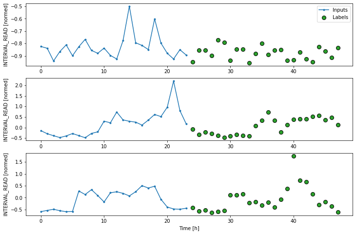
Label column name(s): NoneWe can plot the window to demonstrate the width of the inputs and labels. The labels are the actual values against which predictions will be evaluated. In the plot below, we can see that windowed slices of the data consist of 24 inputs and 24 labels.
Remember that our plots are rendered using an example set of three slices of the training data, but the models will be fitted on the entire training dataframe.
Create a baseline model
As we have done in previous lessons and sections of this lesson, we
will create a naive seasonal baseline forecast that is a
subclass of the tf.keras.Model class. In this case, the
values of the 24 input timesteps for each slice are used as the
predictions for their corresponding label timesteps. This can be seen in
a plot of the model’s predictions, in which the pattern or trend of
predicted values duplicates the pattern or trend of the input
values.
PYTHON
class RepeatBaseline(tf.keras.Model):
  def call(self, inputs):
    return inputs

repeat_baseline = RepeatBaseline()
repeat_baseline.compile(loss=tf.keras.losses.MeanSquaredError(),
                        metrics=[tf.keras.metrics.MeanAbsoluteError()])

multi_val_performance = {}
multi_performance = {}


multi_val_performance['Repeat'] = repeat_baseline.evaluate(multi_window.val)
multi_performance['Repeat'] = repeat_baseline.evaluate(multi_window.test, verbose=0)

print("Baseline performance against validation data:", multi_val_performance["Repeat"])
print("Baseline performance against test data:", multi_performance["Repeat"])

# add a plot
multi_window.plot(repeat_baseline)
OUTPUT
163/163 [==============================] - 1s 3ms/step - loss: 0.4627 - mean_absolute_error: 0.2183
Baseline performance against validation data: [0.46266090869903564, 0.218303844332695]
Baseline performance against test data: [0.5193880200386047, 0.23921075463294983]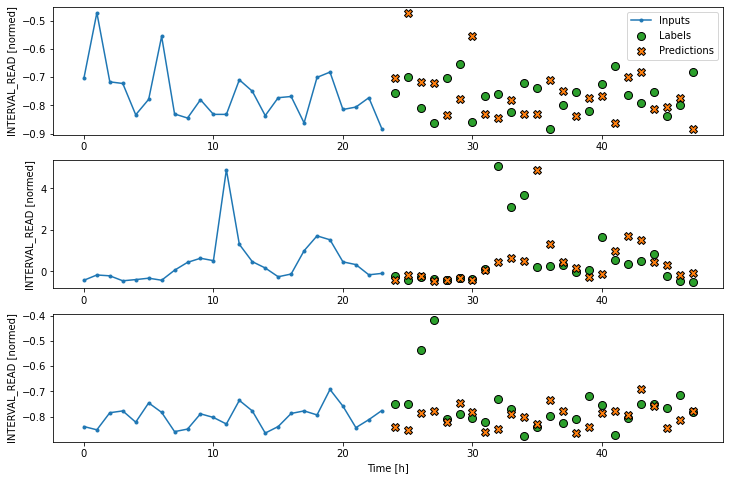
We are now ready to train models. With the addition of creating
layered neural networks using the keras API, all of the
models below will be fitted and evaluated using a workflow similar to
that which we used for the baseline model, above. Rather than repeat the
same code multiple times, before we go any further we will write a
function to encapsulate the process.
The function adds some features to the workflow. As noted above, the loss function acts as a measure of the trade-off between computational costs and accuracy. As the model is fitted, the loss function is used to monitor the model’s efficiency and provides the model an internal mechanism for determining a stopping point.
The compile() method is similar to the above, with the
addition of an optimizer argument. The optimizer is an
algorithm that determines the most efficient weights for each feature as
the model is fitted. In the current example, we are using the
Adam() optimizer that is included as part of the default
TensorFlow library.
Finally, the model is fit using the training dataframe. The data are split using the data window specified in the positional window argument, in our case the single step window defined above. Predictions are validated against the validation data, with the process configured to halt at the point that accuracy no longer improves.
The epochs argument represented the number of times the that the model will work through the entire training dataframe, provided it is not stopped before it reaches that number by the loss function. Note that the MAX_EPOCHS is being manually set in the code block below.
PYTHON
MAX_EPOCHS = 20

def compile_and_fit(model, window, patience=2):
  early_stopping = tf.keras.callbacks.EarlyStopping(monitor='val_loss',
                                                    patience=patience,
                                                    mode='min')

  model.compile(loss=tf.keras.losses.MeanSquaredError(),
                optimizer=tf.keras.optimizers.Adam(),
                metrics=[tf.keras.metrics.MeanAbsoluteError()])

  history = model.fit(window.train, epochs=MAX_EPOCHS,
                      validation_data=window.val,
                      callbacks=[early_stopping])
  return history
With the data window and the compile_and_fit function in
place, we can fit and evaluate models as in the previous section, by
stacking layers of processes into a machine learning pipeline using the
keras API.
Multi step linear
Compared with the single step linear model, the model for forecasting
multiple timesteps requires some additional layers in order to flatten
and reshape the data. In the definition below, the first
Lambda layer flattens the input data using an inline
function. The units argument in the Dense layer is
set dynamically, based on the product of the label_width and the number
of features in the dataset. Finally, the model output is reshaped to
match the input data.
PYTHON
num_features = train_df.shape[1]

multi_linear_model = tf.keras.Sequential([
    tf.keras.layers.Lambda(lambda x: x[:, -1:, :]),
    tf.keras.layers.Dense(OUT_STEPS*num_features,
                          kernel_initializer=tf.initializers.zeros()),
    tf.keras.layers.Reshape([OUT_STEPS, num_features])
])

history = compile_and_fit(multi_linear_model, multi_window)

multi_val_performance['Linear'] = multi_linear_model.evaluate(multi_window.val)
multi_performance['Linear'] = multi_linear_model.evaluate(multi_window.test, verbose=0)

print("Linear performance against validation data:", multi_val_performance["Linear"])
print("Linear performance against test data:", multi_performance["Linear"])

# add a plot
multi_window.plot(multi_linear_model)
OUTPUT
Epoch 10/20
574/574 [==============================] - 1s 1ms/step - loss: 0.3417 - mean_absolute_error: 0.2890 - val_loss: 0.3035 - val_mean_absolute_error: 0.2805
163/163 [==============================] - 0s 929us/step - loss: 0.3035 - mean_absolute_error: 0.2805
Linear performance against validation data: [0.30350184440612793, 0.28051623702049255]
Linear performance against test data: [0.339562326669693, 0.28846967220306396]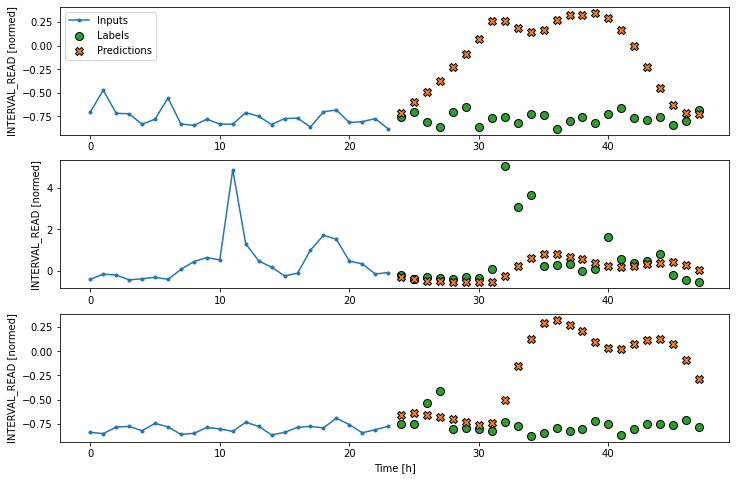
Dense neural network
Similar to the definition of the dense model for single step
forecasts, the definition of the multi-step dense model adds a
Dense layer to the preceeding linear model pipeline. The
activation function is again relu, and the units argument
is increased to 512. The unit argument specifies the shape of the output
that is passed to the next layer.
PYTHON
multi_dense_model = tf.keras.Sequential([
    tf.keras.layers.Lambda(lambda x: x[:, -1:, :]),
    tf.keras.layers.Dense(512, activation='relu'),
    tf.keras.layers.Dense(OUT_STEPS*num_features,
                          kernel_initializer=tf.initializers.zeros()),
    tf.keras.layers.Reshape([OUT_STEPS, num_features])
])

history = compile_and_fit(multi_dense_model, multi_window)

multi_val_performance['Dense'] = multi_dense_model.evaluate(multi_window.val)
multi_performance['Dense'] = multi_dense_model.evaluate(multi_window.test, verbose=0)

print("Dense performance against validation data:", multi_val_performance["Dense"])
print("Dense performance against test data:", multi_performance["Dense"])

# add a plot
multi_window.plot(multi_dense_model)
OUTPUT
Epoch 19/20
574/574 [==============================] - 3s 5ms/step - loss: 0.2305 - mean_absolute_error: 0.1907 - val_loss: 0.2058 - val_mean_absolute_error: 0.1846
163/163 [==============================] - 1s 3ms/step - loss: 0.2058 - mean_absolute_error: 0.1846
Dense performance against validation data: [0.2058122605085373, 0.184647798538208]
Dense performance against test data: [0.22725100815296173, 0.19131870567798615]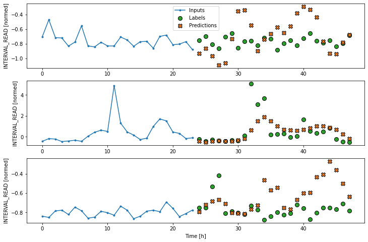
Convolution neural network
For the multi-step convolution neural network model, the first
Dense layer of the previous multi-step dense model is
replaced with a one dimensional convolution layer. The arguments to this
layer include the number of filters, in this case 256, and the kernal
size, which specifies the width of the convolution window.
PYTHON
CONV_WIDTH = 3
multi_conv_model = tf.keras.Sequential([
    tf.keras.layers.Lambda(lambda x: x[:, -CONV_WIDTH:, :]),
    tf.keras.layers.Conv1D(256, activation='relu', kernel_size=(CONV_WIDTH)),
    tf.keras.layers.Dense(OUT_STEPS*num_features,
                          kernel_initializer=tf.initializers.zeros()),
    tf.keras.layers.Reshape([OUT_STEPS, num_features])
])

history = compile_and_fit(multi_conv_model, multi_window)

multi_val_performance['Conv'] = multi_conv_model.evaluate(multi_window.val)
multi_performance['Conv'] = multi_conv_model.evaluate(multi_window.test, verbose=0)

print("CNN performance against validation data:", multi_val_performance["Conv"])
print("CNN performance against test data:", multi_performance["Conv"])

# add a plot
multi_window.plot(multi_conv_model)
OUTPUT
Epoch 17/20
574/574 [==============================] - 1s 2ms/step - loss: 0.2273 - mean_absolute_error: 0.1913 - val_loss: 0.2004 - val_mean_absolute_error: 0.1791
163/163 [==============================] - 0s 1ms/step - loss: 0.2004 - mean_absolute_error: 0.1791
CNN performance against validation data: [0.20042525231838226, 0.17912138998508453]
CNN performance against test data: [0.2245914489030838, 0.18907274305820465]
Recurrent neural network (LSTM)
Recall that the recurrent neural network model maintains an internal
state based on consecutive inputs. For this reason, the
lamba function used so far to flatten the model input is
not necessary in this case. Instead, a single Long Short-Term Memory
(LSTM) layer processes the mode input that is passed to the
Dense layer. The position units argument of 32
specifies the shape of the output. The return_sequences
argument is here set to false so that the internal state will be
maintained until the final input timestep.
PYTHON
multi_lstm_model = tf.keras.Sequential([
    tf.keras.layers.LSTM(32, return_sequences=False),
    tf.keras.layers.Dense(OUT_STEPS*num_features,
                          kernel_initializer=tf.initializers.zeros()),
    tf.keras.layers.Reshape([OUT_STEPS, num_features])
])

history = compile_and_fit(multi_lstm_model, multi_window)


multi_val_performance['LSTM'] = multi_lstm_model.evaluate(multi_window.val)
multi_performance['LSTM'] = multi_lstm_model.evaluate(multi_window.test, verbose=0)

print("LSTM performance against validation data:", multi_val_performance["LSTM"])
print("LSTM performance against test data:", multi_performance["LSTM"])

# add a plot
multi_window.plot(multi_lstm_model)
Epoch 20/20
574/574 [==============================] - 5s 9ms/step - loss: 0.1990 - mean_absolute_error: 0.1895 - val_loss: 0.1760 - val_mean_absolute_error: 0.1786
163/163 [==============================] - 1s 3ms/step - loss: 0.1760 - mean_absolute_error: 0.1786
LSTM performance against validation data: [0.17599913477897644, 0.17859137058258057]
LSTM performance against test data: [0.19873034954071045, 0.18935032188892365]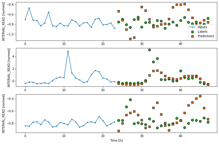
Evaluate
From monitoring the output of the different models for each epoch, we can see that in general all of the multi-step models outperform all of the single step models. Multiple factors can influence model performance, including the size of the dataset, feature engineering, and data normalization. It is not necessarily true that multi-step models will always generally outperform single step models, though that happened to be the case for this dataset.
Similar to the results of the single step models, the convolution neural network performed best overall, though only slightly better than the LSTM model. All three of the neural network models outperformed the baseline and linear models.
OUTPUT
Repeat  : 0.2392
Linear  : 0.2885
Dense   : 0.1913
Conv    : 0.1891
LSTM    : 0.1894
Finally, the below plot provides a comparison of each model’s performance against both the validation and test dataframes.
PYTHON
x = np.arange(len(multi_performance))
width = 0.3

metric_name = 'mean_absolute_error'
metric_index = multi_lstm_model.metrics_names.index('mean_absolute_error')
val_mae = [v[metric_index] for v in multi_val_performance.values()]
test_mae = [v[metric_index] for v in multi_performance.values()]

plt.bar(x - 0.17, val_mae, width, label='Validation')
plt.bar(x + 0.17, test_mae, width, label='Test')
plt.xticks(ticks=x, labels=multi_performance.keys(),
           rotation=45)
plt.ylabel(f'MAE (average over all times and outputs)')
_ = plt.legend()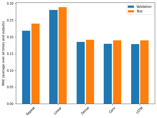
Key Points
- If a label_columns argument is not provided, the data window will forecast all features.