Summary and Setup
This is a new lesson built with The Carpentries Workbench.
The source dataset this used for lesson consists of smart meter power consumption data provided by the Los Alamos Public Utility Department (LADPU) in Los Alamos, New Mexico, USA. In their original format the data have only been processed to remove consumer information. The data contain missing and duplicate values.
The original dataset on which the lesson materials are based is available from Dyrad, LADPU Smart Meter Data, https://doi.org/10.5061/dryad.m0cfxpp2c and has been made available with a CC-0 license:
Souza, Vinicius; Estrada, Trilce; Bashir, Adnan; Mueen, Abdullah (2020), LADPU Smart Meter Data, Dryad, Dataset, https://doi.org/10.5061/dryad.m0cfxpp2c
Data Sets
For this lesson, the data have been modified to support the lesson objectives without requiring a download of the full source dataset from Dryad. Because the source data are large and require cleaning, additional steps have been taken to generate a subset ready for use in this lesson. These steps include:
- Excluding data from meters that were not participating for the full period between January 1, 2014 and December 31, 2019.
- Excluding data from meters that have missing or duplicate readings, or other anomalies.
- Further limiting the included date ranges to exclude common outliers across datasets due to weather events, power outages, or other causes.
- Selection of the final set of 15 data files based on inspection of plots and completeness of the data.
At the outset of a lesson, learners are recommended to create a project directory.
- Download this data file to your computer: Smart meter data subset
- Within a directory on their system for which learners have read and write permissions (user home, desktop, or similar), create a directory named pandas_timeseries.
- In the pandas_timeseries directory, create a subdirectory named data. Unzip the downloaded data into this directory.
- In the pandas_timeseries directory, create two more directories, scripts and figures.
Throughout the lesson, we will be creating scripts in the scripts directory. If using Jupyter Notebooks, be sure to navigate to this directory before creating new notebooks!
Software Setup
Details
The lesson is written in Python. We recommend the Anaconda Python distribution, which is available for all operating systems and comes with most of the necessary libraries installed. Information on how to download and install for different operating systems is available from the Anaconda website.
There are different options for running a Python environment.
The Anaconda distribution recommended above includes Jupyter Notebook, which is a browser-based electronic notebook environment that supports Python, R, and other languages.There are two ways that you can launch a notebook server. The first option is to run the application from the Anaconda Navigator:
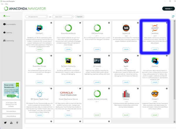
- Launch Anaconda Navigator using your operating system’s application launcher.
- The Navigator is a utility for managing environments, libraries, and
applications. Find the Jupyter Notebook application and click on the
Launch button to start a notebook server:
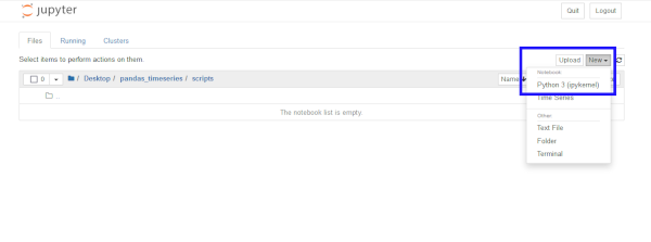
- The Jupyter Notebook server will open up a file navigator in your
home directory of your operating system. Click through to navigate to
the project scripts directory created in the setup, above.
Click on New and select Python 3 to create a Jupyter
Notebook in that directory.
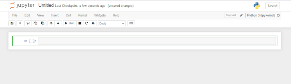
- A new “Untitled” notebook will open up. When you see an empty
notebook cell you are ready to go!
A second option is to use a command line client.
- Open the default command line utility for your operating system. For Mac and many Linux systems, this will be the Terminal app. On Windows, it is recommended to launch either the CMD.exe Prompt or the Powershell Prompt from the Navigator.
- Use the
cdor change directory command to navigate to the scripts subdirectory of the project directory created in the setup section above.
cd ~/Desktop/pandas_timeseries/scriptsLaunch a Jupyter Notebook server using the
jupyter notebookcommand. When the server launches, information similar to the below will appear in the console: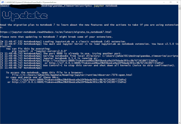
The Jupyter Notebook application will also open in a web browser. Click on New and select Python 3 to create a Jupyter Notebook in that directory.
A new “Untitled” notebook will open up. When you see an empty notebook cell you are ready to go!
When you are finished working, after closing the Jupyter browser interface, be sure to also stop the server using
CONTROL-C.
- Open a shell and enter
python3
Install the TensorFlow library
The lesson uses Google’s TensorFlow machine learning
library throughout. This library is not included in the default Anaconda
distribution, but can be installed through the Navigator. With the
Navigator open as described above:
- Click on the Environments tab in the left sidebar.
- From the drop down menu select “Not Installed.”
- Enter “tensorflow” in the search box.
- The search will return several packages, some of which are dependencies for installing TensorFlow. You only need to check the box next to “tensorflow,” as any required dependencies will be installed along with TensorFlow.
- Click the Update index button to install. You may need to restart Anaconda before using the new library.