Feature Engineering
Last updated on 2023-08-25 | Edit this page
Overview
Questions
- How do you prepare time-series data for machine learning?
Objectives
- Extract datetime elements from a Pandas datetime index.
Introduction
Machine learning methods can fall into two broad categories
- supervised
- unsupervised.
In both cases, the affect or influence of one or more features of an observation are analyzed to determine their effect on a result. The result in this case is termed a label. In supervised learning techniques, models are trained using pre-labeled data. The labels in this case act as a ground truth against which a model’s performance can be compared and evaluated.
In an unsupervised learning process, models are trained using data for which ground truth labels have not been identified. Ground truth in these cases is determined statistically.
Throughout this lesson we are going to focus on unsupervised machine learning techniques to forecast power consumption.
About the code
The code for this and other sections of this lesson is based on time-series forecasting examples, tutorials, and other documentation available from the TensorFlow project. Per the documentation, materials available from the TensorFlow GitHub site published using an Apache 2.0 license.
Google Inc. (2023) TensorFlow Documentation. Retrieved from https://github.com/tensorflow/docs/blob/master/README.md.
Features
The data we used in a separate lesson on modeling time-series forecasts, and which we will continue to use here, include a handful of variables:
- INTERVAL_TIME
- METER_FID
- START_READ
- END_READ
- INTERVAL_READ
In these previous analyses, the only variable used for forecasting power consumption were INTERVAL_READ and INTERVAL_TIME. Going forward, we can capitalize on the efficiency and accuracy of machine learning methods via feature engineering. That is, we want to identify and include as many time-based features as possible that may be relevant to power consumption. For example, though some of our previous models accounted for seasonal trends in the data, other factors that influence power consumption were more difficult to include in our models:
- Day of the week
- Business days, weekends, and holidays
- Season
While some of these features were implicit in the data - for example, power consumption during the US summer notably increased - making these features explicit in our data can result in more accurate machine learning models, with more predictive power.
In this section, we demonstrate a process for extracting these features from a datetime index. The dataset output at the end of this section will be used throughout the rest of this lesson for making forecasts.
Read data
To begin with, import the necessary libraries. We will introduce some new libraries in later sections, but here we only need a handful of libraries to pre-process our daa.
Next we read the data, and set and sort the datetime index.
PYTHON
fp = "../../data/ladpu_smart_meter_data_07.csv"
df = pd.read_csv(fp)
df.set_index(pd.to_datetime(df["INTERVAL_TIME"]), inplace=True)
df.sort_index(inplace=True)

print(df.info())
print(df.index)
OUTPUT
<class 'pandas.core.frame.DataFrame'>
DatetimeIndex: 105012 entries, 2017-01-01 00:00:00 to 2019-12-31 23:45:00
Data columns (total 5 columns):
 #   Column         Non-Null Count   Dtype
---  ------         --------------   -----
 0   INTERVAL_TIME  105012 non-null  object
 1   METER_FID      105012 non-null  int64
 2   START_READ     105012 non-null  float64
 3   END_READ       105012 non-null  float64
 4   INTERVAL_READ  105012 non-null  float64
dtypes: float64(3), int64(1), object(1)
memory usage: 4.8+ MB
None

DatetimeIndex(['2017-01-01 00:00:00', '2017-01-01 00:15:00',
               '2017-01-01 00:30:00', '2017-01-01 00:45:00',
               '2017-01-01 01:00:00', '2017-01-01 01:15:00',
               '2017-01-01 01:30:00', '2017-01-01 01:45:00',
               '2017-01-01 02:00:00', '2017-01-01 02:15:00',
               ...
               '2019-12-31 21:30:00', '2019-12-31 21:45:00',
               '2019-12-31 22:00:00', '2019-12-31 22:15:00',
               '2019-12-31 22:30:00', '2019-12-31 22:45:00',
               '2019-12-31 23:00:00', '2019-12-31 23:15:00',
               '2019-12-31 23:30:00', '2019-12-31 23:45:00'],
              dtype='datetime64[ns]', name='INTERVAL_TIME', length=105012, freq=None)
We will forecasting hourly power consumption in later sections, so we need to resample the data to an hourly frequency here.
PYTHON
hourly_readings = pd.DataFrame(df.resample("h")["INTERVAL_READ"].sum())
print(hourly_readings.info())
print(hourly_readings.head())
OUTPUT
<class 'pandas.core.frame.DataFrame'>
DatetimeIndex: 26280 entries, 2017-01-01 00:00:00 to 2019-12-31 23:00:00
Freq: H
Data columns (total 1 columns):
# Column Non-Null Count Dtype
--- ------ -------------- -----
0 INTERVAL_READ 26280 non-null float64
dtypes: float64(1)
memory usage: 410.6 KB
None
INTERVAL_READ
INTERVAL_TIME
2017-01-01 00:00:00 1.4910
2017-01-01 01:00:00 0.3726
2017-01-01 02:00:00 0.3528
2017-01-01 03:00:00 0.3858
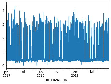
2017-01-01 04:00:00 0.4278A plot of the entire dataset is somewhat noisy, though seasonal trends are apparent.
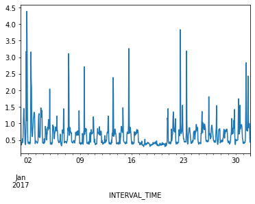
Ploting hourly consumption for the month of January, 2017, is less noisy though there are no obvious trends in the data.
Finally, before manipulating the data we can inspect for anomalies or
outliers using descriptive statistics. Even though we only have a single
variable to describe in our current dataset, the
transpose() method used below is useful in cases where you
want to tabulate descriptive statistics for multiple variables.
OUTPUT
                 count      mean       std  min     25%     50%    75%     max
INTERVAL_READ  26280.0  0.624122  0.405971  0.0  0.3714  0.4818  0.756  4.3872
The max value of 4.3872 may seem like an outlier,
considering that 75% of INTERVAL_READ values are 0.4818 or less.
However, a look back up to our first plot indicates peak power
consumption over a relatively short time period in the middle of the
year. For now we will accept this max value as reasonable.
Add datetime features
Most of the features that we will add to the data are attributes of datetime objects in Pandas. We can extract them using their attribute names:
PYTHON
print("hour:", hourly_readings.head().index.hour)
print("day of the month:", hourly_readings.head().index.day)
print("day of week:", hourly_readings.head().index.day_of_week)
print("day of year:", hourly_readings.head().index.day_of_year)
print("day name:", hourly_readings.head().index.day_name())
print("week of year:",hourly_readings.head().index.week)
print("month:", hourly_readings.head().index.month)
print("year", hourly_readings.head().index.year)
OUTPUT
hour: Int64Index([0, 1, 2, 3, 4], dtype='int64', name='INTERVAL_TIME')

day of the month: Int64Index([1, 1, 1, 1, 1], dtype='int64', name='INTERVAL_TIME')

day of week: Int64Index([6, 6, 6, 6, 6], dtype='int64', name='INTERVAL_TIME')

day of year: Int64Index([1, 1, 1, 1, 1], dtype='int64', name='INTERVAL_TIME')

day name: Index(['Sunday', 'Sunday', 'Sunday', 'Sunday', 'Sunday'], dtype='object', name='INTERVAL_TIME')

week of year: Int64Index([52, 52, 52, 52, 52], dtype='int64', name='INTERVAL_TIME')

month: Int64Index([1, 1, 1, 1, 1], dtype='int64', name='INTERVAL_TIME')

year Int64Index([2017, 2017, 2017, 2017, 2017], dtype='int64', name='INTERVAL_TIME')
We can add these attributes as new features. Out of the attributes shown above, we are only going to add a few numeric types and a full date string.
PYTHON
hourly_readings['hour'] = hourly_readings.index.hour
hourly_readings['day_month'] = hourly_readings.index.day
hourly_readings['day_week'] = hourly_readings.index.day_of_week
hourly_readings['month'] = hourly_readings.index.month
hourly_readings['date'] = hourly_readings.index.to_series().apply(lambda x: x.strftime("%Y-%m-%d"))

print(hourly_readings.info())
print(hourly_readings.head())
print(hourly_readings.tail())
OUTPUT
<class 'pandas.core.frame.DataFrame'>
DatetimeIndex: 26280 entries, 2017-01-01 00:00:00 to 2019-12-31 23:00:00
Freq: H
Data columns (total 6 columns):
 #   Column         Non-Null Count  Dtype
---  ------         --------------  -----
 0   INTERVAL_READ  26280 non-null  float64
 1   hour           26280 non-null  int64
 2   day_month      26280 non-null  int64
 3   day_week       26280 non-null  int64
 4   month          26280 non-null  int64
 5   date           26280 non-null  object
dtypes: float64(1), int64(4), object(1)
memory usage: 1.4+ MB
None

                     INTERVAL_READ  hour  ...  month        date
INTERVAL_TIME                             ...
2017-01-01 00:00:00         1.4910     0  ...      1  2017-01-01
2017-01-01 01:00:00         0.3726     1  ...      1  2017-01-01
2017-01-01 02:00:00         0.3528     2  ...      1  2017-01-01
2017-01-01 03:00:00         0.3858     3  ...      1  2017-01-01
2017-01-01 04:00:00         0.4278     4  ...      1  2017-01-01

[5 rows x 6 columns]

                     INTERVAL_READ  hour  ...  month        date
INTERVAL_TIME                             ...
2019-12-31 19:00:00         0.7326    19  ...     12  2019-12-31
2019-12-31 20:00:00         0.7938    20  ...     12  2019-12-31
2019-12-31 21:00:00         0.7878    21  ...     12  2019-12-31
2019-12-31 22:00:00         0.7716    22  ...     12  2019-12-31
2019-12-31 23:00:00         0.4986    23  ...     12  2019-12-31

[5 rows x 6 columns]
Another feature than can influence power consumption is whether a
given day is a business day, a weekend, or a holiday. For our purposes,
since our data only span three years there may not be enough holidays to
include those as a specific feature. However, we can include US federal
holidays in a customized calendar of business days using Pandas’
holiday and offsets methods.
Note that while this example uses the US federal holiday calendar, Pandas includes holidays and other business day offsets for other regions and locales.
PYTHON
from pandas.tseries.holiday import USFederalHolidayCalendar
from pandas.tseries.offsets import CustomBusinessDay

us_bus = CustomBusinessDay(calendar=USFederalHolidayCalendar())

# Set the business day date range to the start and end dates of our data
us_business_days = pd.bdate_range('2017-01-01', '2019-12-31', freq=us_bus)

hourly_readings["business_day"] = pd.to_datetime(hourly_readings["date"]).isin(us_business_days)
print(hourly_readings.info())
OUTPUT
<class 'pandas.core.frame.DataFrame'>
DatetimeIndex: 26280 entries, 2017-01-01 00:00:00 to 2019-12-31 23:00:00
Freq: H
Data columns (total 7 columns):
 #   Column         Non-Null Count  Dtype
---  ------         --------------  -----
 0   INTERVAL_READ  26280 non-null  float64
 1   hour           26280 non-null  int64
 2   day_month      26280 non-null  int64
 3   day_week       26280 non-null  int64
 4   month          26280 non-null  int64
 5   date           26280 non-null  object
 6   business_day   26280 non-null  bool
dtypes: bool(1), float64(1), int64(4), object(1)
memory usage: 1.4+ MB
None
We want to pass numeric data types to the machine learning processes covered in later sections, so we’ll convert the boolean (True and False) values for business_day to integers (1 for True and 0 for False).
PYTHON
hourly_readings = hourly_readings.astype({"business_day": "int"})
print(hourly_readings.dtypes)
OUTPUT
INTERVAL_READ    float64
hour               int64
day_month          int64
day_week           int64
month              int64
date              object
day_sin          float64
day_cos          float64
business_day       int32
dtype: object
Sine and cosine transformation
Finally, we can apply a sine and cosine transformation to some of the datetime features to more effectively represent the cyclic or periodic nature of specific time frequencies.
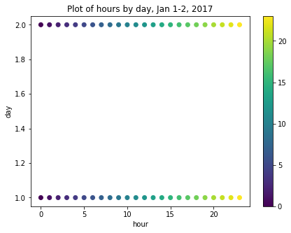
For example, though we have added an hour feature, the data are ordinal. That is, the values for each hour go from 1-24 in order, but hours as an ordinal feature don’t express a cyclic relationship relative to the idea that 1:00 AM of a given date is, time-wise, more or less similar to 1:00 AM of the day before or after. For example, the figure below is a scatter plot of hours per day for January 1-2, 2017, in which ordinal hour “values” are plotted against ordinal day “values.” The overlap we might expect from one day ending and another beginning is not represented.
We can use sine and cosine transformations to add features that capture this characteristic of time. First, we create a timestamp series based on the datetime index.
OUTPUT
Float64Index([1483228800.0, 1483232400.0, 1483236000.0, 1483239600.0,
              1483243200.0, 1483246800.0, 1483250400.0, 1483254000.0,
              1483257600.0, 1483261200.0,
              ...
              1577800800.0, 1577804400.0, 1577808000.0, 1577811600.0,
              1577815200.0, 1577818800.0, 1577822400.0, 1577826000.0,
              1577829600.0, 1577833200.0],
             dtype='float64', name='INTERVAL_TIME', length=26280)
Since timestamps are counted per second, next we want to calculate the number of timestamps in a day and in a year. These values are then applied to sine and cosine transformations of each timestamp value. The transformed values are added as new features to the dataset.
Note that we could use a similar process for weeks, or other datetime elements.
PYTHON
day = 24*60*60
year = (365.2425)*day

hourly_readings['day_sin'] = np.sin(ts_s * (2 * np.pi / day))
hourly_readings['day_cos'] = np.cos(ts_s * (2 * np.pi / day))
hourly_readings['year_sin'] = np.sin(ts_s * (2 * np.pi / year))
hourly_readings['year_cos'] = np.cos(ts_s * (2 * np.pi / year))

print(hourly_readings.info())
OUTPUT
<class 'pandas.core.frame.DataFrame'>
DatetimeIndex: 26280 entries, 2017-01-01 00:00:00 to 2019-12-31 23:00:00
Freq: H
Data columns (total 9 columns):
 #   Column         Non-Null Count  Dtype
---  ------         --------------  -----
 0   INTERVAL_READ  26280 non-null  float64
 1   hour           26280 non-null  int64
 2   day_month      26280 non-null  int64
 3   day_week       26280 non-null  int64
 4   month          26280 non-null  int64
 5   date           26280 non-null  object
 6   business_day   26280 non-null  bool
 7   day_sin        26280 non-null  float64
 8   day_cos        26280 non-null  float64
dtypes: bool(1), float64(3), int64(4), object(1)
memory usage: 1.8+ MB
None
If we now plot the transformed values for January 1-2, 2017, we can see that the plot has a clock-like appearance and that the values for the different hours overlap. In fact, although this is only a plot of the first 48 hours, we could plot the entire dataset and the plot would look the same.
fig, ax = plt.subplots(figsize=(7, 5))
sp = ax.scatter(hourly_readings[:48]['day_sin'],
                hourly_readings[:48]['day_cos'],
                c = hourly_readings[:48]['hour'])
ax.set(
    xlabel="sin(hour)",
    ylabel="cos(hour)",
    title="Plot of hours by day, Jan 1-2, 2017"
)
_ = fig.colorbar(sp)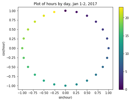
Export data to CSV
At this point, we have added several datetime features to our dataset using datetime attributes. We have additionally used these attributes to add sine and cosine transformed hour features, and a boolean feature indicating whether or not any given day in the dataset is a business day.
Rather than redo this process for the remaining sections of this lesson, we will export the current dataset for later use. The file will be saved to the data directory referenced in the Setup section of this lesson.
Key Points
- Use sine and cosine transformations to represent the periodic or cyclical nature of time-series data.