Introduction
Overview
Teaching: 20 min
Exercises: 10 minQuestions
What kinds of diseases can be observed in chest X-rays?
What is pleural effusion?
Objectives
Gain awareness of the NIH ChestX-ray dataset.
Load a subset of labelled chest X-rays.
Chest X-rays
Chest X-rays are frequently used in healthcare to view the heart, lungs, and bones of patients. On an X-ray, broadly speaking, bones appear white, soft tissue appears grey, and air appears black. The images can show details such as:
- Lung conditions, for example pneumonia, emphysema, or air in the space around the lung.
- Heart conditions, such as heart failure or heart valve problems.
- Bone conditions, such as rib or spine fractures
- Medical devices, such as pacemaker, defibrillators and catheters. X-rays are often taken to assess whether these devices are positioned correctly.
In recent years, organisations like the National Institutes of Health have released large collections of X-rays, labelled with common diseases. The goal is to stimulate the community to develop algorithms that might assist radiologists in making diagnoses, and to potentially discover other findings that may have been overlooked.
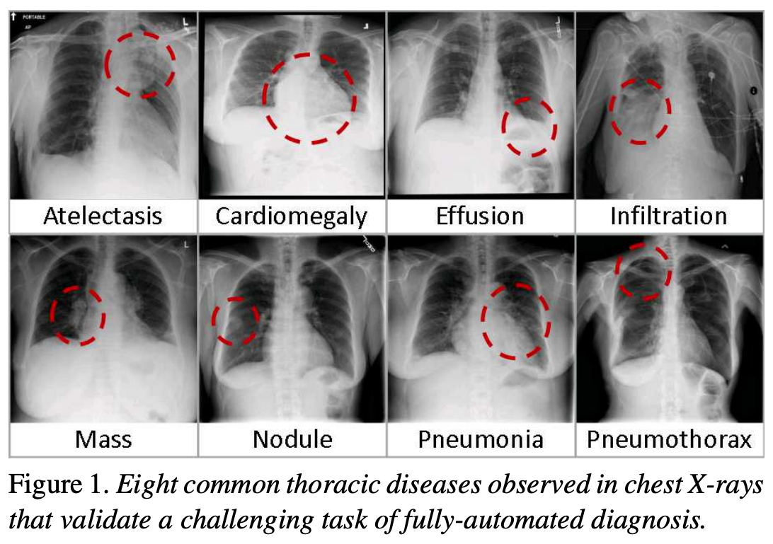
The following figure is from a study by Xiaosong Wang et al. It illustrates eight common diseases that the authors noted could be be detected and even spatially-located in front chest x-rays with the use of modern machine learning algorithms.
Pleural effusion
Thin membranes called “pleura” line the lungs and facilitate breathing. Normally there is a small amount of fluid present in the pleura, but certain conditions can cause excess build-up of fluid. This build-up is known as pleural effusion, sometimes referred to as “water on the lungs”.
Causes of pleural effusion vary widely, ranging from mild viral infections to serious conditions such as congestive heart failure and cancer. In an upright patient, fluid gathers in the lowest part of the chest, and this build up is visible to an expert.
For the remainder of this lesson, we will develop an algorithm to detect pleural effusion in chest X-rays. Specifically, using a set of chest X-rays labelled as either “normal” or “pleural effusion”, we will train a neural network to classify unseen chest X-rays into one of these classes.
Loading the dataset
The data that we are going to use for this project consists of 350 “normal” chest X-rays and 350 X-rays that are labelled as showing evidence pleural effusion. These X-rays are a subset of the public NIH ChestX-ray dataset.
Xiaosong Wang, Yifan Peng, Le Lu, Zhiyong Lu, Mohammadhadi Bagheri, Ronald Summers, ChestX-ray8: Hospital-scale Chest X-ray Database and Benchmarks on Weakly-Supervised Classification and Localization of Common Thorax Diseases, IEEE CVPR, pp. 3462-3471, 2017
Let’s begin by loading the dataset.
# The glob module finds all the pathnames matching a specified pattern
from glob import glob
import os

# If your dataset is compressed, unzip with:
# !unzip chest_xrays.zip

# Define folders containing images
data_path = os.path.join("chest_xrays")
effusion_path = os.path.join(data_path, "effusion", "*.png")
normal_path = os.path.join(data_path, "normal", "*.png")

# Create list of files
effusion_list = glob(effusion_path)
normal_list = glob(normal_path)

print('Number of cases with pleural effusion: ', len(effusion_list))
print('Number of normal cases: ', len(normal_list))
Number of cases with pleural effusion:  350
Number of normal cases:  350
Key Points
Algorithms can be used to detect disease in chest X-rays.
Visualisation
Overview
Teaching: 20 min
Exercises: 10 minQuestions
How does an image with pleural effusion differ from one without?
How is image data represented in a NumPy array?
Objectives
Visually compare normal X-rays with those labelled with pleural effusion.
Understand how to use NumPy to store and manipulate image data.
Compare a slice of numerical data to its corresponding image.
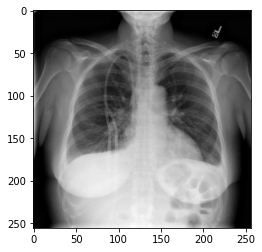
Visualising the X-rays
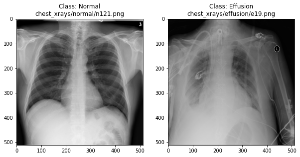
In the previous section, we set up a dataset comprising 700 chest X-rays. Half of the X-rays are labelled “normal” and half are labelled as “pleural effusion”. Let’s take a look at some of the images.
# cv2 is openCV, a popular computer vision library
import cv2
from matplotlib import pyplot as plt
import random

def plot_example(example, label, loc):
    image = cv2.imread(example)
    im = ax[loc].imshow(image)
    title = f"Class: {label}\n{example}"
    ax[loc].set_title(title)

fig, ax = plt.subplots(1, 2)
fig.set_size_inches(10, 10)

# Plot a "normal" record
plot_example(random.choice(normal_list), "Normal", 0)

# Plot a record labelled with effusion
plot_example(random.choice(effusion_list), "Effusion", 1)
Can we detect effusion?
Run the following code to flip a coin to select an x-ray from our collection.
print("Effusion or not?")

# flip a coin
coin_flip = random.choice(["Effusion", "Normal"])
if coin_flip == "Normal":
    fn = random.choice(normal_list)
else:
    fn = random.choice(effusion_list)

# plot the image
image = cv2.imread(fn)
plt.imshow(image)
Show the answer:
# Jupyter doesn't allow us to print the image until the cell has run,
# so we'll print in a new cell.
print(f"The answer is: {coin_flip}!")
Exercise
A) Manually classify 10 X-rays using the coin flip code. Make a note of your predictive accuracy (hint: for a reminder of the formula for accuracy, check the solution below).
Solution
A) Accuracy is the fraction of predictions that were correct (correct predictions / total predictions). If you made 10 predictions and 5 were correct, your accuracy is 50%.
How does a computer see an image?
Consider an image as a matrix in which the value of each pixel corresponds to a number that determines a tone or color. Let’s load one of our images:
import numpy as np

file_idx = 56
example = normal_list[file_idx]
image = cv2.imread(example)

print(image.shape)
(512, 512, 3)
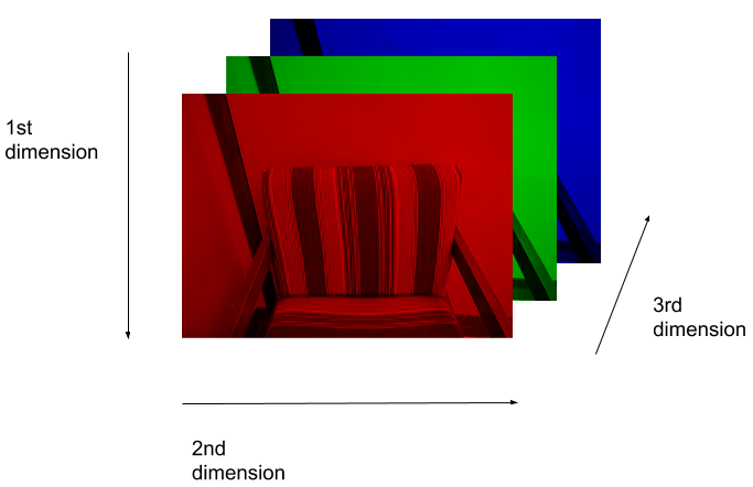
Here we see that the image has 3 dimensions. The first dimension is height (512 pixels) and the second is width (also 512 pixels). The presence of a third dimension indicates that we are looking at a color image (“RGB”, or Red, Green, Blue).
For more detail on image representation in Python, take a look at the Data Carpentry course on Image Processing with Python. The following image is reproduced from the section on Image Representation.
For simplicity, we’ll instead load the images in greyscale. A greyscale image has two dimensions: height and width. Greyscale images have only one channel. Most greyscale images are 8 bits per channel or 16 bits per channel. For a greyscale image with 8 bits per channel, each value in the matrix represents a tone between black (0) and white (255).
image = cv2.imread(example, cv2.IMREAD_GRAYSCALE)
print(image.shape)
(512, 512)
Let’s briefly display the matrix of values, and then see how these same values are rendered as an image.
# Print a 10 by 10 chunk of the matrix
print(image[35:45, 30:40])
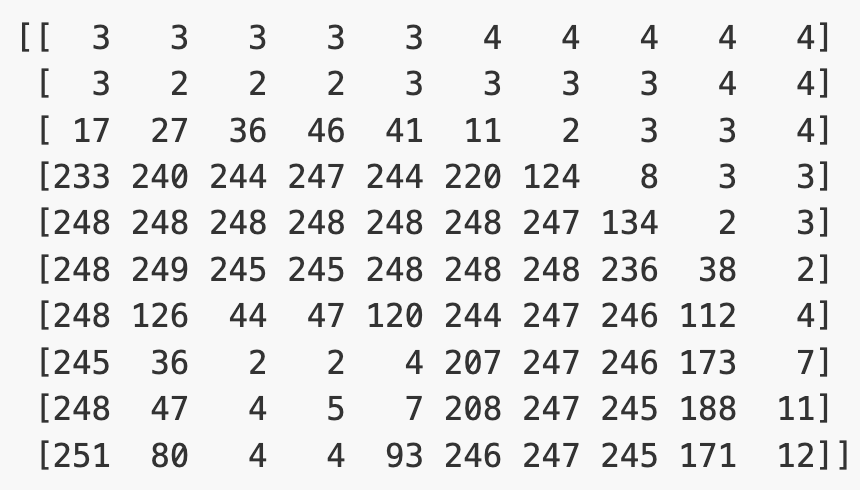
# Plot the same chunk as an image
plt.imshow(image[35:45, 30:40], cmap='gray', vmin=0, vmax=255)
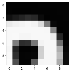
Image pre-processing
In the next episode, we’ll be building and training a model. Let’s prepare our data for the modelling phase. For convenience, we’ll begin by loading all of the images and corresponding labels and assigning them to a list.
# create a list of effusion images and labels
dataset_effusion = [cv2.imread(fn, cv2.IMREAD_GRAYSCALE) for fn in effusion_list]
label_effusion = np.ones(len(dataset_effusion))

# create a list of normal images and labels
dataset_normal = [cv2.imread(fn, cv2.IMREAD_GRAYSCALE) for fn in normal_list]
label_normal = np.zeros(len(dataset_normal))

# Combine the lists
dataset = dataset_effusion + dataset_normal
labels = np.concatenate([label_effusion, label_normal])
Let’s also downsample the images, reducing the size from (512, 512) to (256,256).
# Downsample the images from (512,512) to (256,256)
dataset = [cv2.resize(img, (256,256)) for img in dataset]

# Check the size of the reshaped images
print(dataset[0].shape)

# Normalize the data
# Subtract the mean, divide by the standard deviation.
for i in range(len(dataset)):
  dataset[i] = (dataset[i] - np.average(dataset[i], axis= (0, 1))) / np.std(dataset[i], axis= (0, 1))
(256, 256)
Finally, we’ll convert our dataset from a list to an array. We are expecting it to be (700, 256, 256). That is 700 images (350 effusion cases and 350 normal), each with a dimension of 256 by 256.
dataset = np.asarray(dataset, dtype=np.float32)
print(f"Matrix Dimensions: {dataset.shape}")
(700, 256, 256)
We could plot the images by indexing them on dataset, e.g., we can plot the first image in the dataset with:
idx = 0
vals = dataset[idx].flatten()
plt.imshow(dataset[idx], cmap='gray', vmin=min(vals), vmax=max(vals))
Key Points
In NumPy, RGB images are usually stored as 3-dimensional arrays.
Data preparation
Overview
Teaching: 20 min
Exercises: 10 minQuestions
What is the purpose of data augmentation?
What types of transform can be applied in data augmentation?
Objectives
Generate an augmented dataset
Partition data into training and test sets.
Partitioning into training and test sets
As we have done in previous projects, we will want to split our data into subsets for training and testing. The training set is used for building our model and our test set is used for evaluation.
To ensure reproducibility, we should set the random state of the splitting method. This means that Python’s random number generator will produce the same “random” split in future.
from sklearn.model_selection import train_test_split

# Our Tensorflow model requires the input to be:
# [batch, height, width, n_channels]
# So we need to add a dimension to the dataset and labels.
#
# Ellipsis (...) is shorthand for selecting with ":" across dimensions.
# np.newaxis expands the selection by one dimension.
dataset = dataset[..., np.newaxis]
labels = labels[..., np.newaxis]

# Create training and test sets
dataset_train, dataset_test, labels_train, labels_test = train_test_split(dataset, labels, test_size=0.15, random_state=42)

# Create a validation set
dataset_train, dataset_val, labels_train, labels_val = train_test_split(dataset_train, labels_train, test_size=0.15, random_state=42)

print("No. images, x_dim, y_dim, colors) (No. labels, 1)\n")
print(f"Train: {dataset_train.shape}, {labels_train.shape}")
print(f"Validation: {dataset_val.shape}, {labels_val.shape}")
print(f"Test: {dataset_test.shape}, {labels_test.shape}")
No. images, x_dim, y_dim, colors) (No. labels, 1)

Train: (505, 256, 256, 1), (505, 1)
Validation: (90, 256, 256, 1), (90, 1)
Test: (105, 256, 256, 1), (105, 1)
Data Augmentation
We have a small dataset, which increases the chance of overfitting our model. If our model is overfitted, it becomes less able to generalize to data outside the training data.
To artificially increase the size of our training set, we can use ImageDataGenerator. This function generates new data by applying random transformations to our source images while our model is training.
from tensorflow.keras.preprocessing.image import ImageDataGenerator

# Define what kind of transformations we would like to apply
# such as rotation, crop, zoom, position shift, etc
datagen = ImageDataGenerator(
    rotation_range=0,
    width_shift_range=0,
    height_shift_range=0,
    zoom_range=0,
    horizontal_flip=False)
For the sake of interest, let’s take a look at some examples of the augmented images!
# specify path to source data
path = os.path.join("chest_xrays")
batch_size=5

val_generator = datagen.flow_from_directory(
        path, color_mode="rgb",
        target_size=(256, 256),
        batch_size=batch_size)

def plot_images(images_arr):
    fig, axes = plt.subplots(1, 5, figsize=(20,20))
    axes = axes.flatten()
    for img, ax in zip(images_arr, axes):
        ax.imshow(img.astype('uint8'))
    plt.tight_layout()
    plt.show()

augmented_images = [val_generator[0][0][0] for i in range(batch_size)]
plot_images(augmented_images)
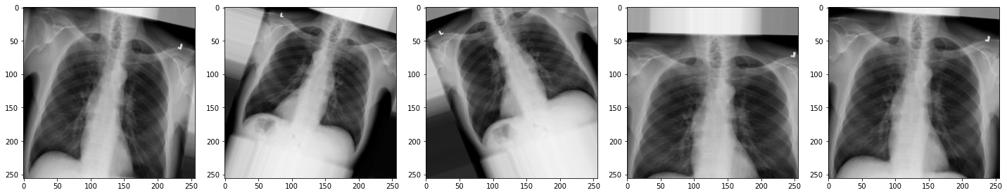
The images look a little strange, but that’s the idea! When our model sees something unusual in real-life, it will be better adapted to deal with it.
Now we have some data to work with, let’s start building our model.
Key Points
Data augmentation can help to avoid overfitting.
Neural networks
Overview
Teaching: 20 min
Exercises: 10 minQuestions
What is a neural network?
What are the characteristics of a dense layer?
What is an activation function?
What is a convolutional neural network?
Objectives
Become familiar with key components of a neural network.
Create the architecture for a convolutational neural network.
What is a neural network?
An artificial neural network, or just “neural network”, is a broad term that describes a family of machine learning models that are (very!) loosely based on the neural circuits found in biology.
The smallest building block of a neural network is a single neuron. A typical neuron receives inputs (x1, x2, x3) which are multiplied by learnable weights (w1, w2, w3), then summed with a bias term (b). An activation function (f) determines the neuron output.
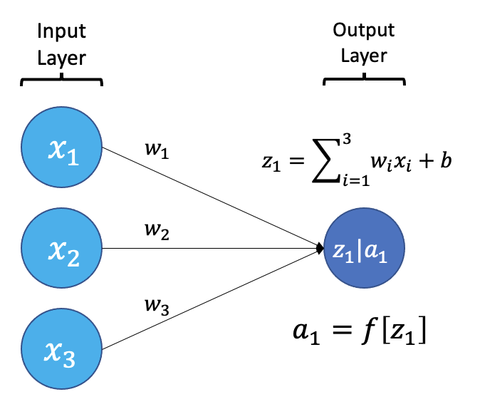
From a high level, a neural network is a system that takes input values in an “input layer”, processes these values with a collection of functions in one or more “hidden layers”, and then generates an output such as a prediction. The network has parameters that are systematically tweaked to allow pattern recognition.
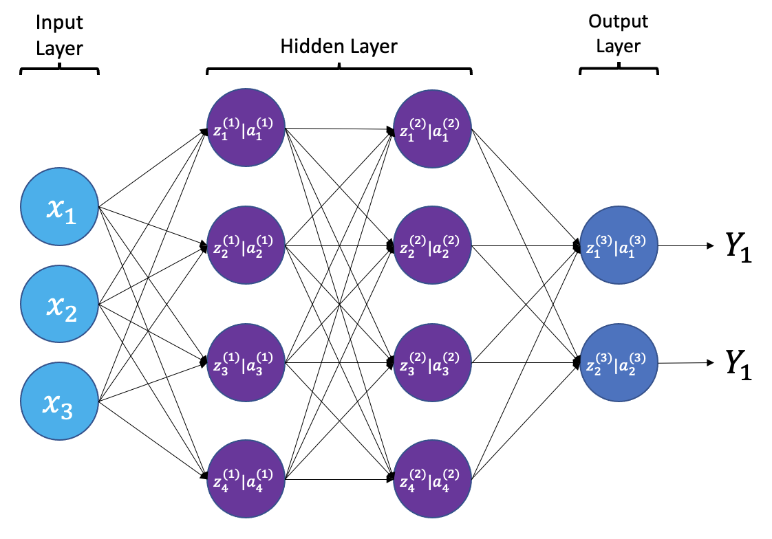
The layers shown in the network above are “dense” or “fully connected”. Each neuron is connected to all neurons in the preceeding layer. Dense layers are a common building block in neural network architectures.
“Deep learning” is an increasingly popular term used to describe certain types of neural network. When people talk about deep learning they are typically referring to more complex network designs, often with a large number of hidden layers.
Activation Functions
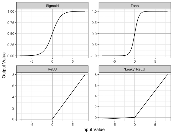
Part of the concept of a neural network is that each neuron can either be ‘active’ or ‘inactive’. This notion of activity and inactivity is attempted to be replicated by so called activation functions. The original activation function was the sigmoid function (related to its use in logistic regression). This would make each neuron’s activation some number between 0 and 1, with the idea that 0 was ‘inactive’ and 1 was ‘active’.
As time went on, different activation functions were used. For example the tanh function (hyperbolic tangent function), where the idea is a neuron can be active in both a positive capacity (close to 1), a negative capacity (close to -1) or can be inactive (close to 0).
The problem with both of these is that they suffered from a problem called model saturation. This is where very high or very low values are put into the activation function, where the gradient of the line is almost flat. This leads to very slow learning rates (it can take a long time to train models with these activation functions).
Another very popular activation function that tries to tackle this is the rectified linear unit (ReLU) function. This has 0 if the input is negative (inactive) and just gives back the input if it is positive (a measure of how active it is - the metaphor gets rather stretched here). This is much faster at training and gives very good performance, but still suffers model saturation on the negative side. Researchers have tried to get round this with functions like ‘leaky’ ReLU, where instead of returning 0, negative inputs are multiplied by a very small number.
Convolutional neural networks
Convolutional neural networks (CNNs) are a type of neural network that especially popular for vision tasks such as image recognition. CNNs are very similar to ordinary neural networks, but they have characteristics that make them well suited to image processing.
Just like other neural networks, a CNN typically consists of an input layer, hidden layers and an output layer. The layers of “neurons” have learnable weights and biases, just like other networks.
What makes CNNs special? The name stems from the fact that the architecture includes one or more convolutional layers. These layers apply a mathematical operation called a “convolution” to extract features from arrays such as images.
In a convolutional layer, a matrix of values referred to as a “filter” or “kernel” slides across the input matrix (in our case, an image). As it slides, values are multiplied to generate a new set of values referred to as a “feature map” or “activation map”.
Filters provide a mechanism for emphasising aspects of an input image. For example, a filter may emphasise object edges. See setosa.io for a visual demonstration of the effect of different filters.
Creating a convolutional neural network
Before training a convolutional neural network, we will first need to define the architecture. We can do this using the Keras and Tensorflow libraries.
# Create the architecture of our convolutional neural network, using
# the tensorflow library
from tensorflow.random import set_seed
from tensorflow.keras.layers import Dense, Dropout, Conv2D, MaxPool2D, Input, GlobalAveragePooling2D
from tensorflow.keras.models import Model

# set random seed for reproducibility
set_seed(42)

# Our input layer should match the input shape of our images.
# A CNN takes tensors of shape (image_height, image_width, color_channels)
# We ignore the batch size when describing the input layer
# Our input images are 256 by 256, plus a single colour channel.
inputs = Input(shape=(256, 256, 1))

# Let's add the first convolutional layer
x = Conv2D(filters=8, kernel_size=3, padding='same', activation='relu')(inputs)

# MaxPool layers are similar to convolution layers.
# The pooling operation involves sliding a two-dimensional filter over each channel of feature map and selecting the max values.
# We do this to reduce the dimensions of the feature maps, helping to limit the amount of computation done by the network.
x = MaxPool2D()(x)

# We will add more convolutional layers, followed by MaxPool
x = Conv2D(filters=8, kernel_size=3, padding='same', activation='relu')(x)
x = MaxPool2D()(x)
x = Conv2D(filters=12, kernel_size=3, padding='same', activation='relu')(x)
x = MaxPool2D()(x)
x = Conv2D(filters=12, kernel_size=3, padding='same', activation='relu')(x)
x = MaxPool2D()(x)
x = Conv2D(filters=20, kernel_size=5, padding='same', activation='relu')(x)
x = MaxPool2D()(x)
x = Conv2D(filters=20, kernel_size=5, padding='same', activation='relu')(x)
x = MaxPool2D()(x)
x = Conv2D(filters=50, kernel_size=5, padding='same', activation='relu')(x)

# Global max pooling reduces dimensions back to the input size
x = GlobalAveragePooling2D()(x)

# Finally we will add two "dense" or "fully connected layers".
# Dense layers help with the classification task, after features are extracted.
x = Dense(128, activation='relu')(x)

# Dropout is a technique to help prevent overfitting that involves deleting neurons.
x = Dropout(0.6)(x)

x = Dense(32, activation='relu')(x)

# Our final dense layer has a single output to match the output classes.
# If we had multi-classes we would match this number to the number of classes.
outputs = Dense(1, activation='sigmoid')(x)

# Finally, we will define our network with the input and output of the network
model = Model(inputs=inputs, outputs=outputs)
We can view the architecture of the model:
model.summary()
Model: "model_39"
_________________________________________________________________
 Layer (type)                Output Shape              Param #
=================================================================
 input_9 (InputLayer)        [(None, 256, 256, 1)]     0

 conv2d_59 (Conv2D)          (None, 256, 256, 8)       80

 max_pooling2d_50 (MaxPoolin  (None, 128, 128, 8)      0
 g2D)

 conv2d_60 (Conv2D)          (None, 128, 128, 8)       584

 max_pooling2d_51 (MaxPoolin  (None, 64, 64, 8)        0
 g2D)

 conv2d_61 (Conv2D)          (None, 64, 64, 12)        876

 max_pooling2d_52 (MaxPoolin  (None, 32, 32, 12)       0
 g2D)

 conv2d_62 (Conv2D)          (None, 32, 32, 12)        1308

 max_pooling2d_53 (MaxPoolin  (None, 16, 16, 12)       0
 g2D)

 conv2d_63 (Conv2D)          (None, 16, 16, 20)        6020

 max_pooling2d_54 (MaxPoolin  (None, 8, 8, 20)         0
 g2D)

 conv2d_64 (Conv2D)          (None, 8, 8, 20)          10020

 max_pooling2d_55 (MaxPoolin  (None, 4, 4, 20)         0
 g2D)

 conv2d_65 (Conv2D)          (None, 4, 4, 50)          25050

 global_average_pooling2d_8   (None, 50)               0
 (GlobalAveragePooling2D)

 dense_26 (Dense)            (None, 128)               6528

 dropout_8 (Dropout)         (None, 128)               0

 dense_27 (Dense)            (None, 32)                4128

 dense_28 (Dense)            (None, 1)                 33

=================================================================
Total params: 54,627
Trainable params: 54,627
Non-trainable params: 0
_________________________________________________________________
Key Points
Dense layers, also known as fully connected layers, are an important building block in most neural network architectures. In a dense layer, each neuron is connected to every neuron in the preceeding layer.
Dropout is a method that helps to prevent overfitting by temporarily removing neurons from the network.
The Rectified Linear Unit (ReLU) is an activation function that outputs an input if it is positive, and outputs zero if it is not.
Convolutional neural networks are typically used for imaging tasks.
Training and evaluation
Overview
Teaching: 20 min
Exercises: 10 minQuestions
How do I train a neural network?
Objectives
Train a convolutational neural network for classification.
Evalute the network’s performance on a test set.
Compile and train your model
Now that the model architecture is complete, it is ready to be compiled and trained! The distance between our predictions and the true values is the error or “loss”. The goal of training is to minimise this loss.
Through training, we seek an optimal set of model parameters. Using an optimization algorithm such as gradient descent, our model weights are iteratively updated as each batch of data is processed.
Batch size is the number of training examples processed before the model parameters are updated. An epoch is one complete pass through all of the training data. In an epoch, we use all of the training examples once.
from tensorflow.keras import optimizers
from tensorflow.keras.callbacks import ModelCheckpoint

# Define the network optimization method.
# Adam is a popular gradient descent algorithm
# with adaptive, per-parameter learning rates.
custom_adam = optimizers.Adam()

# Compile the model defining the 'loss' function type, optimization and the metric.
model.compile(loss='binary_crossentropy', optimizer=custom_adam, metrics=['acc'])

# Save the best model found during training
checkpointer = ModelCheckpoint(filepath='best_model.hdf5', monitor='val_loss',
                               verbose=1, save_best_only=True)

# Now train our network!
# steps_per_epoch = len(dataset_train)//batch_size
hist = model.fit(datagen.flow(dataset_train, labels_train, batch_size=32),
                 steps_per_epoch=15,
                 epochs=10,
                 validation_data=(dataset_val, labels_val),
                 callbacks=[checkpointer])
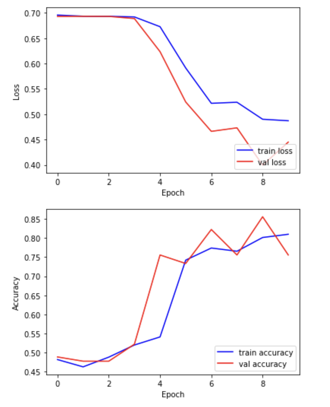
We can now plot the results of the training. “Loss” should drop over successive epochs and accuracy should increase.
plt.plot(hist.history['loss'], 'b-', label='train loss')
plt.plot(hist.history['val_loss'], 'r-', label='val loss')
plt.ylabel('Loss')
plt.xlabel('Epoch')
plt.legend(loc='lower right')
plt.show()

plt.plot(hist.history['acc'], 'b-', label='train accuracy')
plt.plot(hist.history['val_acc'], 'r-', label='val accuracy')
plt.ylabel('Accuracy')
plt.xlabel('Epoch')
plt.legend(loc='lower right')
plt.show()
Evaluating your model on the held-out test set
In this step, we present the unseen test dataset to our trained network and evaluate the performance.
from tensorflow.keras.models import load_model

# Open the best model saved during training
best_model = load_model('best_model.hdf5')
print('\nNeural network weights updated to the best epoch.')
Now that we’ve loaded the best model, we can evaluate the accuracy on our test data.
# We use the evaluate function to evaluate the accuracy of our model in the test group
print(f"Accuracy in test group: {best_model.evaluate(dataset_test, labels_test, verbose=0)[1]}")
Accuracy in test group: 0.80
Key Points
During the training process we iteratively update the model to minimise error.
Explainability
Overview
Teaching: 20 min
Exercises: 10 minQuestions
What is a saliency map?
What aspects of an image contribute to predictions?
Objectives
Review model performance with saliency maps.
Explainability
If a model is making a prediction, many of us would like to know how the decision was reached. Saliency maps - and related approaches - are a popular form of explainability for imaging models.
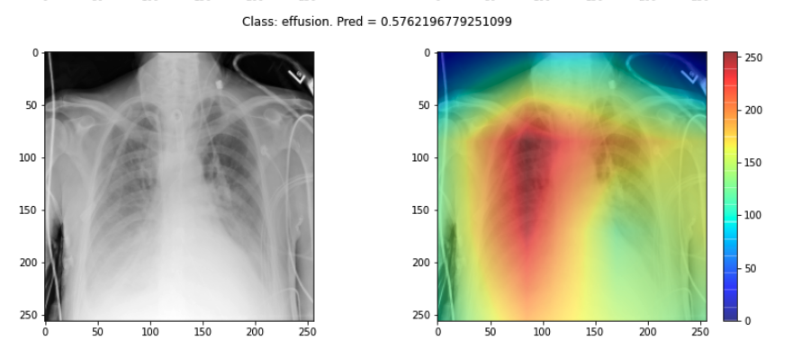
Saliency maps use color to illustrate the extent to which a region of an image contributes to a given decision. Let’s plot some saliency maps for our model:
# !pip install tf_keras_vis
from matplotlib import cm
from tf_keras_vis.gradcam import Gradcam

import numpy as np
from matplotlib import pyplot as plt
from tf_keras_vis.gradcam_plus_plus import GradcamPlusPlus
from tf_keras_vis.scorecam import Scorecam
from tf_keras_vis.utils.scores import CategoricalScore

# Select two differing explainability algorithms
gradcam = GradcamPlusPlus(best_model, clone=True)
scorecam = Scorecam(best_model, clone=True)


def plot_map(cam, classe, prediction, img):
    """
    Plot the image.
    """
    fig, axes = plt.subplots(1,2, figsize=(14, 5))
    axes[0].imshow(np.squeeze(img), cmap='gray')
    axes[1].imshow(np.squeeze(img), cmap='gray')
    heatmap = np.uint8(cm.jet(cam[0])[..., :3] * 255)
    i = axes[1].imshow(heatmap, cmap="jet", alpha=0.5)
    fig.colorbar(i)
    plt.suptitle("Class: {}. Pred = {}".format(classe, prediction))

# Plot each image with accompanying saliency map
for image_id in range(10):
    SEED_INPUT = dataset_test[image_id]
    CATEGORICAL_INDEX = [0]

    layer_idx = 18
    penultimate_layer_idx = 13
    class_idx  = 0

    cat_score = labels_test[image_id]
    cat_score = CategoricalScore(CATEGORICAL_INDEX)
    cam = gradcam(cat_score, SEED_INPUT,
                  penultimate_layer = penultimate_layer_idx,
                  normalize_cam=True)

    # Display the class
    _class = 'normal' if labels_test[image_id] == 0 else 'effusion'
    _prediction = best_model.predict(dataset_test[image_id][np.newaxis, :, ...], verbose=0)

    plot_map(cam, _class, _prediction[0][0], SEED_INPUT)
Sanity checks for saliency maps
While saliency maps may offer us interesting insights about regions of an image contributing to a model’s output, there are suggestions that this kind of visual assessment can be misleading. For example, the following abstract is from a paper entitled “Sanity Checks for Saliency Maps”:
Saliency methods have emerged as a popular tool to highlight features in an input deemed relevant for the prediction of a learned model. Several saliency methods have been proposed, often guided by visual appeal on image data. … Through extensive experiments we show that some existing saliency methods are independent both of the model and of the data generating process. Consequently, methods that fail the proposed tests are inadequate for tasks that are sensitive to either data or model, such as, finding outliers in the data, explaining the relationship between inputs and outputs that the model learned, and debugging the model.
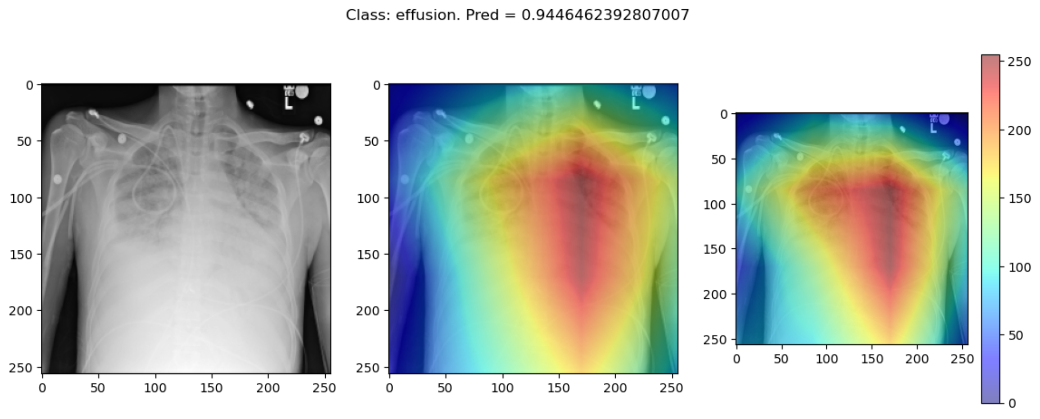
There are multiple methods for producing saliency maps to explain how a particular model is making predictions. The method we have been using is called GradCam++, but how does this method compare to another? Use this code to compare GradCam++ with ScoreCam.
def plot_map2(cam1, cam2, classe, prediction, img):
    """
    Plot the image.
    """
    fig, axes = plt.subplots(1, 3, figsize=(14, 5))
    axes[0].imshow(np.squeeze(img), cmap='gray')
    axes[1].imshow(np.squeeze(img), cmap='gray')
    axes[2].imshow(np.squeeze(img), cmap='gray')
    heatmap1 = np.uint8(cm.jet(cam1[0])[..., :3] * 255)
    heatmap2 = np.uint8(cm.jet(cam2[0])[..., :3] * 255)
    i = axes[1].imshow(heatmap1, cmap="jet", alpha=0.5)
    j = axes[2].imshow(heatmap2, cmap="jet", alpha=0.5)
    fig.colorbar(i)
    plt.suptitle("Class: {}. Pred = {}".format(classe, prediction))

# Plot each image with accompanying saliency map
for image_id in range(10):
    SEED_INPUT = dataset_test[image_id]
    CATEGORICAL_INDEX = [0]

    layer_idx = 18
    penultimate_layer_idx = 13
    class_idx  = 0

    cat_score = labels_test[image_id]
    cat_score = CategoricalScore(CATEGORICAL_INDEX)
    cam = gradcam(cat_score, SEED_INPUT,
                  penultimate_layer = penultimate_layer_idx,
                  normalize_cam=True)
    cam2 = scorecam(cat_score, SEED_INPUT,
                  penultimate_layer = penultimate_layer_idx,
                  normalize_cam=True
                  )

    # Display the class
    _class = 'normal' if labels_test[image_id] == 0 else 'effusion'
    _prediction = best_model.predict(dataset_test[image_id][np.newaxis, : ,...], verbose=0)

    plot_map2(cam, cam2, _class, _prediction[0][0], SEED_INPUT)
Some of the time these methods largely agree:
But some of the time they disagree wildly:
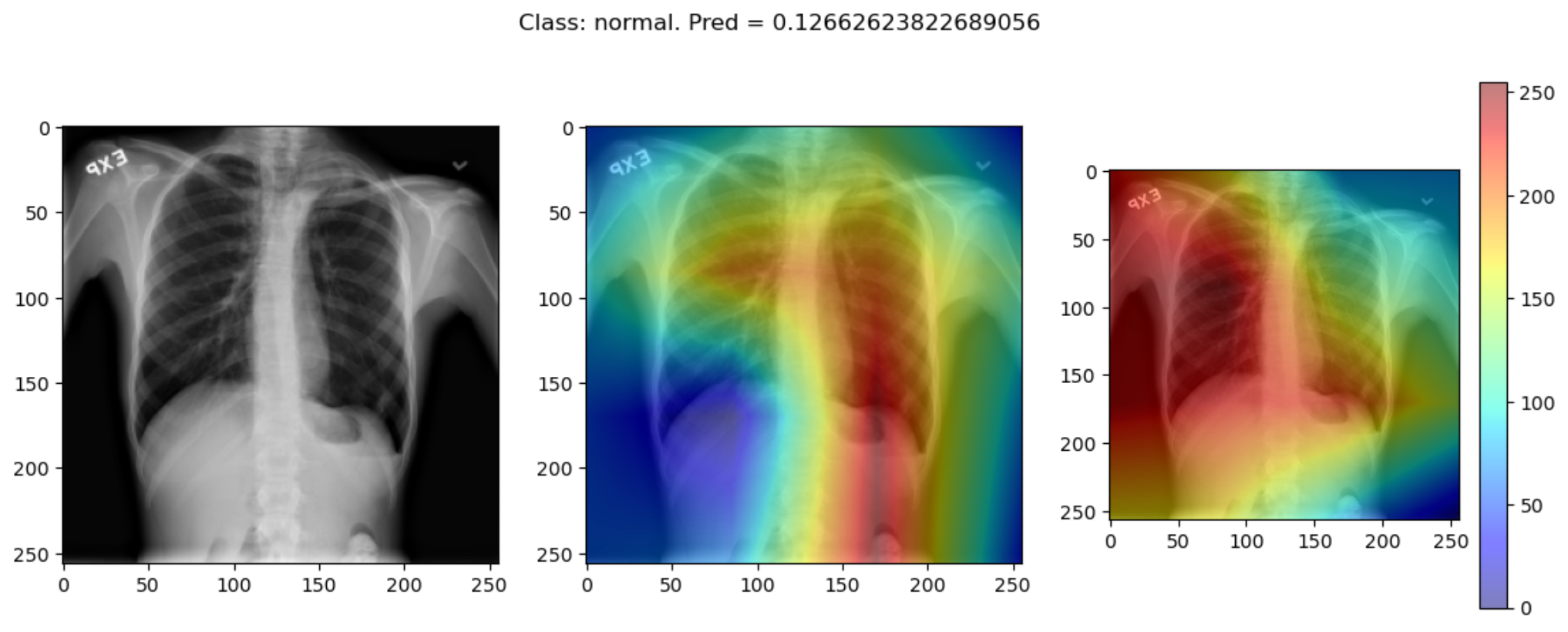
This raises the question, should these algorithms be used at all?
This is part of a larger problem with explainability of complex models in machine learning. The generally accepted answer is to know how your model works and to know how your explainability algorithm works as well as to understand your data.
With these three pieces of knowledge it should be possible to identify algorithms appropriate for your task, and to understand any shortcomings in their approaches.
Key Points
Saliency maps are a popular form of explainability for imaging models.
Saliency maps should be used cautiously.