Explainability
Overview
Teaching: 20 min
Exercises: 10 minQuestions
What is a saliency map?
What aspects of an image contribute to predictions?
Objectives
Review model performance with saliency maps.
Explainability
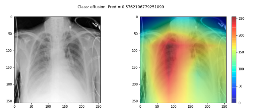
If a model is making a prediction, many of us would like to know how the decision was reached. Saliency maps - and related approaches - are a popular form of explainability for imaging models.
Saliency maps use color to illustrate the extent to which a region of an image contributes to a given decision. Let’s plot some saliency maps for our model:
# !pip install tf_keras_vis
from matplotlib import cm
from tf_keras_vis.gradcam import Gradcam

import numpy as np
from matplotlib import pyplot as plt
from tf_keras_vis.gradcam_plus_plus import GradcamPlusPlus
from tf_keras_vis.scorecam import Scorecam
from tf_keras_vis.utils.scores import CategoricalScore

# Select two differing explainability algorithms
gradcam = GradcamPlusPlus(best_model, clone=True)
scorecam = Scorecam(best_model, clone=True)


def plot_map(cam, classe, prediction, img):
    """
    Plot the image.
    """
    fig, axes = plt.subplots(1,2, figsize=(14, 5))
    axes[0].imshow(np.squeeze(img), cmap='gray')
    axes[1].imshow(np.squeeze(img), cmap='gray')
    heatmap = np.uint8(cm.jet(cam[0])[..., :3] * 255)
    i = axes[1].imshow(heatmap, cmap="jet", alpha=0.5)
    fig.colorbar(i)
    plt.suptitle("Class: {}. Pred = {}".format(classe, prediction))

# Plot each image with accompanying saliency map
for image_id in range(10):
    SEED_INPUT = dataset_test[image_id]
    CATEGORICAL_INDEX = [0]

    layer_idx = 18
    penultimate_layer_idx = 13
    class_idx  = 0

    cat_score = labels_test[image_id]
    cat_score = CategoricalScore(CATEGORICAL_INDEX)
    cam = gradcam(cat_score, SEED_INPUT,
                  penultimate_layer = penultimate_layer_idx,
                  normalize_cam=True)

    # Display the class
    _class = 'normal' if labels_test[image_id] == 0 else 'effusion'
    _prediction = best_model.predict(dataset_test[image_id][np.newaxis, :, ...], verbose=0)

    plot_map(cam, _class, _prediction[0][0], SEED_INPUT)
Sanity checks for saliency maps
While saliency maps may offer us interesting insights about regions of an image contributing to a model’s output, there are suggestions that this kind of visual assessment can be misleading. For example, the following abstract is from a paper entitled “Sanity Checks for Saliency Maps”:
Saliency methods have emerged as a popular tool to highlight features in an input deemed relevant for the prediction of a learned model. Several saliency methods have been proposed, often guided by visual appeal on image data. … Through extensive experiments we show that some existing saliency methods are independent both of the model and of the data generating process. Consequently, methods that fail the proposed tests are inadequate for tasks that are sensitive to either data or model, such as, finding outliers in the data, explaining the relationship between inputs and outputs that the model learned, and debugging the model.
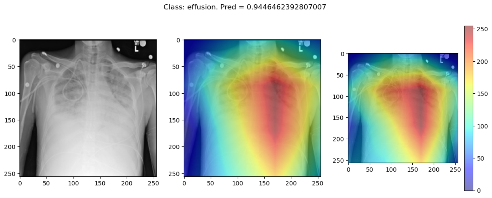
There are multiple methods for producing saliency maps to explain how a particular model is making predictions. The method we have been using is called GradCam++, but how does this method compare to another? Use this code to compare GradCam++ with ScoreCam.
def plot_map2(cam1, cam2, classe, prediction, img):
    """
    Plot the image.
    """
    fig, axes = plt.subplots(1, 3, figsize=(14, 5))
    axes[0].imshow(np.squeeze(img), cmap='gray')
    axes[1].imshow(np.squeeze(img), cmap='gray')
    axes[2].imshow(np.squeeze(img), cmap='gray')
    heatmap1 = np.uint8(cm.jet(cam1[0])[..., :3] * 255)
    heatmap2 = np.uint8(cm.jet(cam2[0])[..., :3] * 255)
    i = axes[1].imshow(heatmap1, cmap="jet", alpha=0.5)
    j = axes[2].imshow(heatmap2, cmap="jet", alpha=0.5)
    fig.colorbar(i)
    plt.suptitle("Class: {}. Pred = {}".format(classe, prediction))

# Plot each image with accompanying saliency map
for image_id in range(10):
    SEED_INPUT = dataset_test[image_id]
    CATEGORICAL_INDEX = [0]

    layer_idx = 18
    penultimate_layer_idx = 13
    class_idx  = 0

    cat_score = labels_test[image_id]
    cat_score = CategoricalScore(CATEGORICAL_INDEX)
    cam = gradcam(cat_score, SEED_INPUT,
                  penultimate_layer = penultimate_layer_idx,
                  normalize_cam=True)
    cam2 = scorecam(cat_score, SEED_INPUT,
                  penultimate_layer = penultimate_layer_idx,
                  normalize_cam=True
                  )

    # Display the class
    _class = 'normal' if labels_test[image_id] == 0 else 'effusion'
    _prediction = best_model.predict(dataset_test[image_id][np.newaxis, : ,...], verbose=0)

    plot_map2(cam, cam2, _class, _prediction[0][0], SEED_INPUT)
Some of the time these methods largely agree:
But some of the time they disagree wildly:
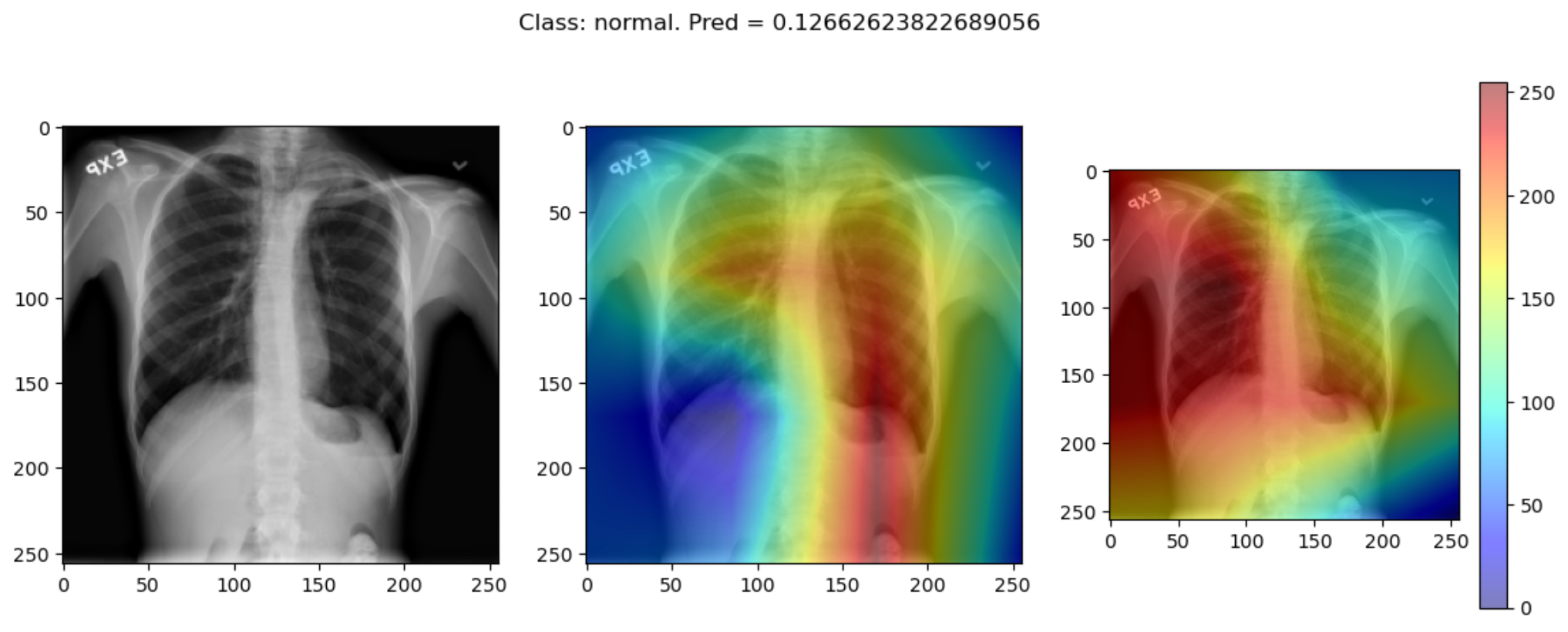
This raises the question, should these algorithms be used at all?
This is part of a larger problem with explainability of complex models in machine learning. The generally accepted answer is to know how your model works and to know how your explainability algorithm works as well as to understand your data.
With these three pieces of knowledge it should be possible to identify algorithms appropriate for your task, and to understand any shortcomings in their approaches.
Key Points
Saliency maps are a popular form of explainability for imaging models.
Saliency maps should be used cautiously.