Training and evaluation
Overview
Teaching: 20 min
Exercises: 10 minQuestions
How do I train a neural network?
Objectives
Train a convolutational neural network for classification.
Evalute the network’s performance on a test set.
Compile and train your model
Now that the model architecture is complete, it is ready to be compiled and trained! The distance between our predictions and the true values is the error or “loss”. The goal of training is to minimise this loss.
Through training, we seek an optimal set of model parameters. Using an optimization algorithm such as gradient descent, our model weights are iteratively updated as each batch of data is processed.
Batch size is the number of training examples processed before the model parameters are updated. An epoch is one complete pass through all of the training data. In an epoch, we use all of the training examples once.
from tensorflow.keras import optimizers
from tensorflow.keras.callbacks import ModelCheckpoint

# Define the network optimization method.
# Adam is a popular gradient descent algorithm
# with adaptive, per-parameter learning rates.
custom_adam = optimizers.Adam()

# Compile the model defining the 'loss' function type, optimization and the metric.
model.compile(loss='binary_crossentropy', optimizer=custom_adam, metrics=['acc'])

# Save the best model found during training
checkpointer = ModelCheckpoint(filepath='best_model.hdf5', monitor='val_loss',
                               verbose=1, save_best_only=True)

# Now train our network!
# steps_per_epoch = len(dataset_train)//batch_size
hist = model.fit(datagen.flow(dataset_train, labels_train, batch_size=32),
                 steps_per_epoch=15,
                 epochs=10,
                 validation_data=(dataset_val, labels_val),
                 callbacks=[checkpointer])
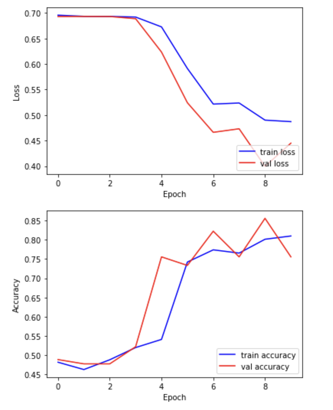
We can now plot the results of the training. “Loss” should drop over successive epochs and accuracy should increase.
plt.plot(hist.history['loss'], 'b-', label='train loss')
plt.plot(hist.history['val_loss'], 'r-', label='val loss')
plt.ylabel('Loss')
plt.xlabel('Epoch')
plt.legend(loc='lower right')
plt.show()

plt.plot(hist.history['acc'], 'b-', label='train accuracy')
plt.plot(hist.history['val_acc'], 'r-', label='val accuracy')
plt.ylabel('Accuracy')
plt.xlabel('Epoch')
plt.legend(loc='lower right')
plt.show()
Evaluating your model on the held-out test set
In this step, we present the unseen test dataset to our trained network and evaluate the performance.
from tensorflow.keras.models import load_model

# Open the best model saved during training
best_model = load_model('best_model.hdf5')
print('\nNeural network weights updated to the best epoch.')
Now that we’ve loaded the best model, we can evaluate the accuracy on our test data.
# We use the evaluate function to evaluate the accuracy of our model in the test group
print(f"Accuracy in test group: {best_model.evaluate(dataset_test, labels_test, verbose=0)[1]}")
Accuracy in test group: 0.80
Key Points
During the training process we iteratively update the model to minimise error.