An introduction to binary response variables
Overview
Teaching: 40 min
Exercises: 20 minQuestions
How can we calculate probabilities of success and failure?
How do we interpret the expectation of a binary variable?
How can we calculate and interpret the odds?
How can we calculate and interpret the log odds?
Objectives
Calculate the probabilities of success and failure given binary data.
Interpret the expectation of a binary variable.
Calculate and interpret the odds of success given binary data.
Calculate and interpret the log odds of success given binary data.
In this lesson we will work with binary outcome variables. That is, variables which can take one of two possible values. For example, these could be $0$ or $1$, “success” or “failure” or “yes” or “no”.
Probabilities and expectation
By analysing binary data, we can estimate the probabilities of success and failure. For example, if we consider individuals between the ages of 55 and 66, we may be interested in the probability that individuals who have once smoked, are still smoking during the NHANES study.
The probability of success is estimated by the proportion of individuals who are still smoking. Similarly, the probability of failure is estimated by the proportion of individuals who are no longer smoking. In this context, we would consider an individual that still smokes a “success” and an individual that no longer smokes a “failure”.
We calculate these values in RStudio through four operations:
- Removing empty rows with
drop_na(); - Subsetting individuals of the appropriate age using
filter(); - Counting the number of individuals in each of the two levels of
SmokeNowusingcount(); - Calculating proportions by dividing the counts by the total number
of non-NA observations using
mutate().
dat %>%
  drop_na(SmokeNow) %>% # there are no empty rows in Age
                        # so we only use drop_na on SmokeNow
  filter(between(Age, 55, 66)) %>%
  count(SmokeNow, name = "n") %>%
  mutate(prop = n/sum(n))
  SmokeNow   n      prop
1       No 359 0.6232639
2      Yes 217 0.3767361
We see that the probability of success is estimated as $0.38$ and the probability
of failure is estimated as $0.62$. In mathematical notation:
$\text{Pr}(\text{SmokeNow} = \text{Yes}) = 0.38$ and $\text{Pr}(\text{SmokeNow} = \text{No}) = 0.62$.
You may have noticed that the probabilities of success and failure add to 1. This is true because there are only two possible outcomes for a binary response variable. Therefore, the probability of success equals 1 minus the probability of failure: $\text{Pr}(\text{Success}) = 1 - \text{Pr}(\text{Failure})$.
In the linear regression lessons, we modelled the expectation of the outcome variable, $E(y)$. In the case of binary variables, we will also work with the expectation of the outcome variable. When $y$ is a binary variable, $E(y)$ is equal to the probability of success. In our example above, $E(y) = \text{Pr}(\text{SmokeNow} = \text{Yes}) = 0.38$.
Exercise
You have been asked to study physical activity (
PhysActive) in individuals with an FEV1 (FEV1) between 3750 and 4250 in the NHANES data.
A) Estimate the probabilitites that someone is or is not physically active for individuals with an FEV1 between 3750 and 4250.
B) What value is $E(\text{PhysActive})$ for individuals with an FEV1 between 3750 and 4250?Solution
A) To obtain the probabilities:
dat %>%
  drop_na(PhysActive) %>%
  filter(between(FEV1, 3750, 4250)) %>%
  count(PhysActive) %>%
  mutate(prop = n/sum(n))
PhysActive n prop 1 No 242 0.3159269 2 Yes 524 0.6840731We therefore estimate the probability of physical activity to be $0.68$ and the probability of no physical activity to be $0.32$.
B) $E(\text{PhysActive}) = \text{Pr}(\text{PhysActive} = \text{Yes}) = 0.68$
Why does $E(y)$ equal the probability of success?
In general, the expectation of a variable equals its probability-weighted mean. This is calculated by taking the sum of all values that a variable can take on, each multiplied by the probability of that value occuring.
In mathematical notation, this is indicated by:
\[E(y) = \sum_i\Big(y_i \times \text{Pr}(y = y_i)\Big)\]In the case of a binary variable, the variable can take one of two values: $0$ and $1$. Therefore, the expectation becomes:
\[E(y) = \sum_i\Big(y_i \times \text{Pr}(y = y_i)\Big) = 0 \times \text{Pr}(y = 0) + 1 \times \text{Pr}(y = 1) = \text{Pr}(y = 1)\]Since “success” is considered $y=1$, the expectation of a binary variable equals the probability of success.
Odds and log odds
Besides probabilities, binary data is often interpreted through odds. The odds are defined as:
[\frac{E(y)}{1-E(y)}.]
Since the expectation of $y$ equals the probability of success, the odds can also be written as:
[\frac{E(y)}{1-E(y)} = \frac{\text{Pr}(\text{Success})}{1-\text{Pr}(\text{Success})} = \frac{\text{Pr}(\text{Success})}{\text{Pr}(\text{Failure})}.]
Therefore, an odds greater than $1$ indicates that the probability of success is greater than the probability of failure. For example, an odds of 1.5 indicates that success is 1.5 times as likely as failure. An odds less than $1$ indicates that the probability of failure is greater than the probability of success. For example, an odds of 0.75 indicates that success is 0.75 times as likely as failure.
Binary outcome variables can be modeled through the log odds. We can see the relationship between the log odds and the expectation in the plot below. As we can see in the plot, a log odds greater than zero is associated with a probability of success greater than 0.5. Likewise, a log odds smaller than 0 is associated with a probability of success less than 0.5.
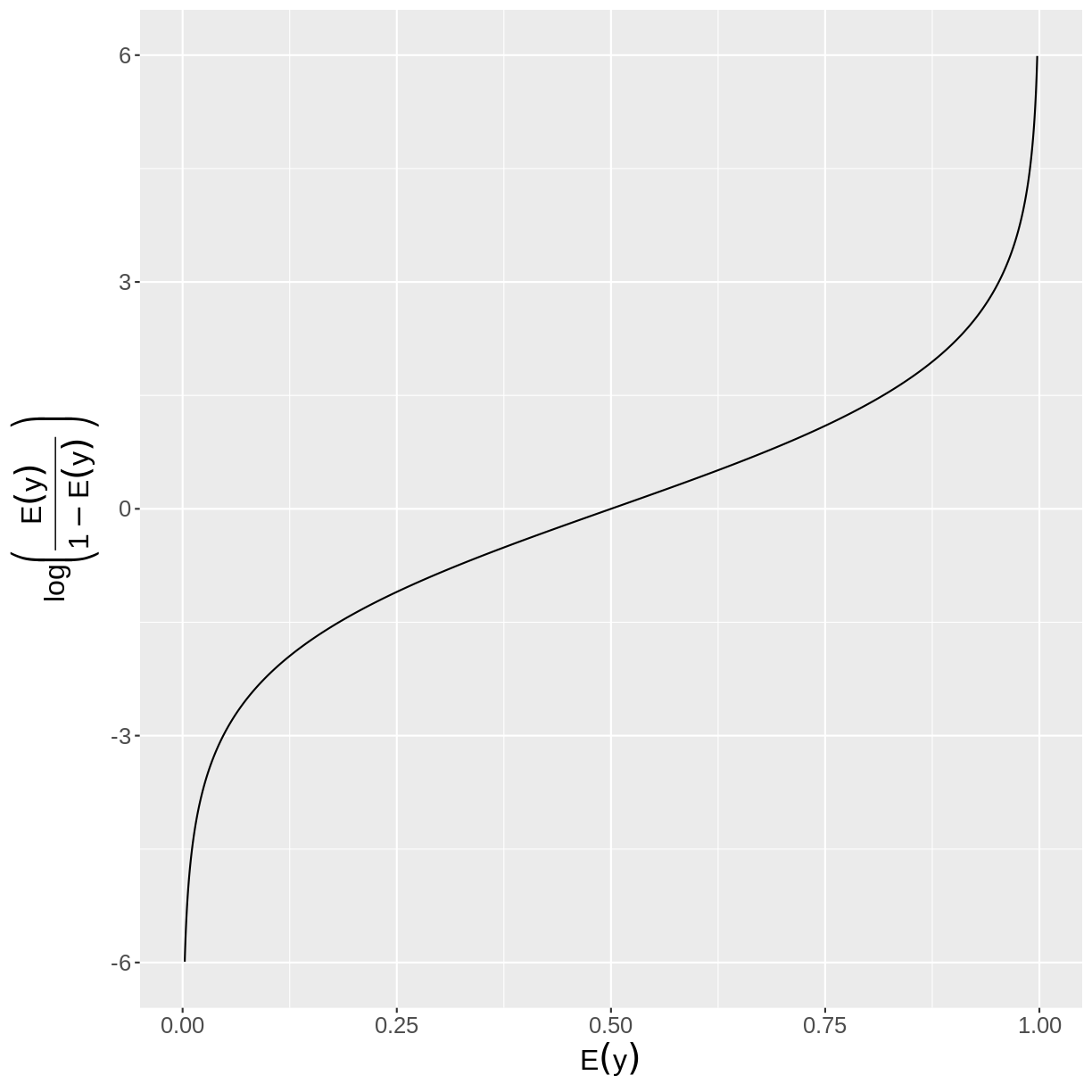
In mathematical notation, the log odds is defined as:
[\text{log}\left(\frac{E(y)}{1-E(y)}\right).]
The interpretation of the probabilities, odds and log odds is summarised in the table below:
| Measure | Turning point | Interpretation |
|---|---|---|
| Probability | 0.5 | Proportion of observations that are successes |
| Odds | 1.0 | How many times more likely is success than failure? |
| Log odds | 0 | If log odds > 0, probability is > 0.5. |
The odds and the log odds can be calculated in RStudio through an
extension of the code that we used to calculate the probabilities.
From our table of probabilities we isolate the row with the probability
of success using filter(). We then calculate the odds and the log odds
using the summarise() function.
dat %>%
  drop_na(SmokeNow) %>%
  filter(between(Age, 55, 66)) %>%
  count(SmokeNow) %>%
  mutate(prop = n/sum(n)) %>%
  filter(SmokeNow == "Yes") %>%
  summarise(odds = prop/(1 - prop),
    log_odds = log(prop/(1 - prop)))
       odds  log_odds
1 0.6044568 -0.503425
Exercise
You have been asked to study physical activity (
PhysActive) in individuals with an FEV1 (FEV1) between 3750 and 4250 in the NHANES data. Calculate the odds and the log odds of physical activity for individuals with an FEV1 between 3750 and 4250. How is the odds interpreted here?Solution
dat %>%
  drop_na(PhysActive) %>%
  filter(between(FEV1, 3750, 4250)) %>%
  count(PhysActive) %>%
  mutate(prop = n/sum(n)) %>%
  filter(PhysActive == "Yes") %>%
  summarise(odds = prop/(1 - prop),
    log_odds = log(prop/(1 - prop)))
odds log_odds 1 2.165289 0.772554Since the odds equal 2.17, we expect individuals with an FEV1 between 3750 and 4250 to be 2.17 times more likely to be physically active than not.
What does $\text{log}()$ do?
The $\text{log}()$ is a transformation used widely in statistics, including in the modelling of binary variables. In general, $\text{log}_a(b)$ tells us to what power we need to raise $a$ to obtain the value $b$.
For example, $2^3 = 2 \times 2 \times 2 = 8$. Therefore, $\text{log}_2(8)=3$, since we raise $2$ to the power of $3$ to obtain 8.
Similarly, $\text{log}_3(81)=4$, since $3^4=81$.
In logistic regression, we use $\text{log}_{e}()$, where $e$ is a mathematical constant. The constant $e$ approximately equals 2.718.
Rather than writing $\text{log}_{e}()$, we write $\text{log}()$ for simplicity.
In R, we can calculate the log using the
log()function. For example, to calculate to what power we need to raise $e$ to obtain $10$:log(10)[1] 2.302585
Key Points
The probabilities of success and failure are estimated as the proportions of participants with a success and failure, respectively.
The expectation of a binary variable equals the probability of success.
The odds equal the ratio of the probability of success and one minus the probability of success. The odds quantify how many times more likely success is than failure.
The log odds are calculated by taking the log of the odds. When the log odds are greater than 0, the probability of success is greater than 0.5.
An introduction to logistic regression
Overview
Teaching: 45 min
Exercises: 45 minQuestions
In what scenario is a logistic regression model useful?
How is the logistic regression model expressed in terms of the log odds?
How is the logistic regression model expressed in terms of the probability of success?
What is the effect of the explanatory variable in terms of the odds?
Objectives
Identify questions that can be addressed with a logistic regression model.
Formulate the model equation in terms of the log odds.
Formulate the model equation in terms of the probability of success.
Express the effect of an explanatory variable in terms of a multiplicative change in the odds.
Scenarios in which logistic regression may be useful
Logistic regression is commonly used, but when is it appropriate to apply this method? Broadly speaking, logistic regression may be suitable when the following conditions hold:
- You seek a model of the relationship between one binary dependent variable and at least one continuous or categorical explanatory variable.
- Your data and logistic regression model do not violate the assumptions of the logistic regression model. We will cover these assumptions in the final episode of this lesson.
Exercise
A colleague has started working with the NHANES data set. They approach you for advice on the use of logistic regression on this data. Assuming that the assumptions of the logistic regression model hold, which of the following questions could potentially be tackled with a logistic regression model? Think closely about the outcome and explanatory variables, between which a relationship will be modelled to answer the research questions.
A) Does home ownership (whether a participant’s home is owned or rented) vary across income bracket in the general US population?
B) Is there an association between BMI and pulse rate in the general US population?
C) Do participants with diabetes on average have a higher weight than participants without diabetes?Solution
A) The outcome variable is home ownership and the explanatory variable is income bracket. Since home ownership is a binary outcome variable, logistic regression could be a suitable way to investigate this question.
B) Since both variables are continuous, logistic regression is not suitable for this question.
C) The outcome variable is weight and the explanatory variable is diabetes. Since the outcome variable is continuous and the explanatory variable is binary, this question is not suited for logistic regression. Note that an alternative question, with diabetes as the outcome variable and weight as the explanatory variable, could be investigated using logistic regression.
The logistic regression model equation in terms of the log odds
The logistic regression model can be described by the following equation:
[\text{log}\left(\frac{E(y)}{1-E(y)}\right) = \beta_0 + \beta_1 \times x_1.]
The right-hand side of the equation has the same form as that for simple linear regression. So we will first interpret the left-hand side of the equation. The outcome variable is denoted by $y$. Logistic regression models the log odds of $E(y)$, which we encountered in the previous episode.
The log odds can be denoted by $\text{logit()}$ for simplicity, giving us the following equation:
[\text{logit}(E(y)) = \beta_0 + \beta_1 \times x_1.]
As we learned in the previous episode, the expectation of $y$ is another way of referring to the probability of success. We also learned that the probability of success equals one minus the probability of failure. Therefore, the left-hand side of our equation can be denoted by:
[\text{logit}(E(y)) = \text{log}\left(\frac{E(y)}{1-E(y)}\right) = \text{log}\left(\frac{\text{Pr}(y=1)}{1-\text{Pr}(y=1)}\right) = \text{log}\left(\frac{\text{Pr}(y=1)}{\text{Pr}(y=0)}\right).]
This leads us to interpreting $\text{logit}(E(y))$ as the log odds of $y=1$ (or success).
In the logistic regression model equation, the expectation of $y$ is a function of $\beta_0$ and $\beta_1 \times x_1$. The intercept is denoted by $\beta_0$ - this is the log odds when the explanatory variable, $x_1$, equals 0. The effect of our explanatory variable is denoted by $\beta_1$ - for every one-unit increase in $x_1$, the log odds changes by $\beta_1$.
Before fitting the model, we have $y$ and $x_1$ values for each observation in our data. For example, suppose we want to model the relationship between diabetes and BMI. $y$ would represent diabetes ($y=1$ if a participant has diabetes and $y=0$ otherwise). $x_1$ would represent BMI. After we fit the model, R will return to us values of $\beta_0$ and $\beta_1$ - these are estimated using our data.
Exercise
We are asked to study the association between BMI and diabetes. We are given the following equation of a logistic regression model to use:
\(\text{logit}(E(y)) = \beta_0 + \beta_1 \times x_1\).
Match the following components of this logistic regression model to their descriptions:
- $\text{logit}(E(y))$
- ${\beta}_0$
- $x_1$
- ${\beta}_1$
A) The log odds of having diabetes, for a particular value of BMI.
B) The expected change in the log odds of having diabetes with a one-unit increase in BMI.
C) The expected log odds of having diabetes when the BMI equals 0.
D) A specific value of BMI.Solution
A) 1
B) 4
C) 2
D) 3
The logistic regression model equation in terms of the probability of success
Alternatively, the logistic regression model can be expressed in terms of probabilities of success. This formula is obtained by using the inverse function of $\text{logit}()$, denoted by $\text{logit}^{-1}()$. In general terms, an inverse function “reverses” the original function, returning the input value. This means that $\text{logit}^{-1}(\text{logit}(E(y))) = E(y)$. Taking the inverse logit on both sides of the logistic regression equation introduced above, we obtain:
[\begin{align}
\text{logit}^{-1}(\text{logit}(E(y))) & = \text{logit}^{-1}(\beta_0 + \beta_1 \times x_1)
E(y) & = \text{logit}^{-1}(\beta_0 + \beta_1 \times x_1).
\end{align}]
The advantage of this formulation is that our output is in terms of probabilities of success. We will encounter this formulation when plotting the results of our models.
Exercise
We are asked to study the association between age and smoking status. We are given the following equation of a logistic regression model to use:
\(E(y) = \text{logit}^{-1}(\beta_0 + \beta_1 \times x_1).\)
Match the following components of this logistic regression model to their descriptions:
- $E(y)$
- ${\beta}_0$
- $x_1$
- ${\beta}_1$
- $\text{logit}^{-1}()$
A) A specific value of age.
B) The expected probability of being a smoker for a particular value of age.
C) The inverse logit function.
D) The expected log odds of still smoking given an age of 0.
E) The expected change in the log odds with a one-unit difference in age.Solution
A) 3
B) 1
C) 5
D) 2
E) 4
The multiplicative change in the odds ratio
As we have seen above, the effect of an explanatory variable is expressed in terms of the log odds of success. For every unit increase in $x_1$, the log odds changes by $\beta_1$. For a different interpretation, we can express the effect of an explanatory variable in terms of multiplicative change in the odds of success.
Specifically, $\frac{\text{Pr}(y=1)}{\text{Pr}(y=0)}$ is multiplied by $e^{\beta_1}$ for every unit increase in $x_1$. For example, if $\frac{\text{Pr}(y=1)}{\text{Pr}(y=0)} = 0.2$ at $x=0$ and $\beta_1 = 2$, then at $x=1$ $\frac{\text{Pr}(y=1)}{\text{Pr}(y=0)} = 0.2 \times e^2 = 1.48$. In general terms, this relationship is expressed as:
| [\frac{\text{Pr}(y=1 | x=a+1)}{\text{Pr}(y=0 | x=a+1)} = \frac{\text{Pr}(y=1 | x=a)}{\text{Pr}(y=0 | x=a)} \times e^{\beta_1},] |
where $\frac{\text{Pr}(y=1|x=a)}{\text{Pr}(y=0|x=a)}$ is read as the “odds of $y$ being $1$ given $x$ being $a$”. In this context, $a$ is any value that $x$ can take on.
Importantly, this means that the change in the odds of success is not linear. The change depends on the odds $\frac{\text{Pr}(y=1|x=a)}{\text{Pr}(y=0|x=a)}$. We will exemplify this in the challenge below.
Exercise
We are given the following odds of success: $\frac{\text{Pr}(y=1|x=2)}{\text{Pr}(y=0|x=2)} = 0.4$ and $\frac{\text{Pr}(y=1|x=6)}{\text{Pr}(y=0|x=6)} = 0.9$. We are also given an estimate of the effect of an explanatory variable: $\beta_1 = 1.2$.
A) Calculate the expected multiplicative change in the odds of success. An exponential can be calculated in R using
exp(), e.g. $e^2$ is obtained withexp(2).
B) Calculate $\frac{\text{Pr}(y=1|x=3)}{\text{Pr}(y=0|x=3)}$.
C) Calculate $\frac{\text{Pr}(y=1|x=7)}{\text{Pr}(y=0|x=7)}$.
D) By how much did the odds of success change when going from $x=2$ to $x=3$? And when going from $x=6$ to $x=7$?Solution
A) $e^{1.2} = 3.32.$ We can obtain this in R as follows:
exp(1.2)[1] 3.320117B) $\frac{\text{Pr}(y=1|x=3)}{\text{Pr}(y=0|x=3)} = 0.4 \times 3.32 = 1.328$
C) $\frac{\text{Pr}(y=1|x=7)}{\text{Pr}(y=0|x=7)} = 0.9 \times 3.32 = 2.988$
D) $1.328 - 0.4 = 0.928$ and $2.988 - 0.9 = 2.088$. So the second change is greater than the first change.
If you are interested in the reason why this multiplicative change exists, see the callout box below.
Why does the odds change by a factor of $e^{\beta_1}$?
To understand the reason behind the multiplicative relationship, we need to look at the ratio of two odds:
\[\frac{\frac{\text{Pr}(y=1|x=a+1)}{\text{Pr}(y=0|x=a+1)}}{\frac{\text{Pr}(y=1|x=a)}{\text{Pr}(y=0|x=a)}}.\]Let’s call this ratio $A$. The numerator of $A$ is the odds of success when $x=a+1$. The denominator of $A$ is the odds of success when $x=a$. Therefore, if $A>1$ then the odds of success is greater when $x=a+1$. Alternatively, if $A<1$, then the odds of success is smaller when $x=a+1$.
Taking the exponential of a log returns the logged value, i.e. $e^{\text{log}(a)} = a$. Therefore, we can express the odds in terms of the exponentiated model equation:
\[\text{log}\left(\frac{\text{Pr}(y=1)}{\text{Pr}(y=0)}\right) = \beta_0 + \beta_1 \times x_1 \Leftrightarrow \frac{\text{Pr}(y=1)}{\text{Pr}(y=0)} = e^{\beta_0 + \beta_1 \times x_1}.\]The ratio of two odds can thus be expressed in terms of the exponentiated model equations:
\[\frac{\frac{\text{Pr}(y=1|x=a+1)}{\text{Pr}(y=0|x=a+1)}}{\frac{\text{Pr}(y=1|x=a)}{\text{Pr}(y=0|x=a)}} = \frac{e^{\beta_0 + \beta_1 \times (a+1)}}{e^{\beta_0 + \beta_1\times a}}.\]Since the exponential of a sum is the product of the exponentiated components:
\[\frac{\frac{\text{Pr}(y=1|x=a+1)}{\text{Pr}(y=0|x=a+1)}}{\frac{\text{Pr}(y=1|x=a)}{\text{Pr}(y=0|x=a)}} = \frac{e^{\beta_0} \times e^{(\beta_1 \times a)} \times e^{\beta_1}}{e^{\beta_0} \times e^{(\beta_1 \times a)}}.\]This can then be simplified by crossing out components found in the numerator and the denominator:
\[\frac{\frac{\text{Pr}(y=1|x=a+1)}{\text{Pr}(y=0|x=a+1)}}{\frac{\text{Pr}(y=1|x=a)}{\text{Pr}(y=0|x=a)}} = e^{\beta_1}.\]Finally, bringing the denominator from the left-hand side to the right-hand side:
\[\frac{\text{Pr}(y=1|x=a+1)}{\text{Pr}(y=0|x=a+1)} = \frac{\text{Pr}(y=1|x=a)}{\text{Pr}(y=0|x=a)} \times e^{\beta_1}.\]
Key Points
Logistic regression requires one binary dependent variable and one or more continuous or categorical explanatory variables.
The model equation in terms of the log odds is $\text{logit}(E(y)) = \beta_0 + \beta_1 \times x_1$.
The model equation in terms of the probability of success is $E(y) = \text{logit}^{-1}(\beta_0 + \beta_1 \times x_1)$.
The odds is multiplied by $e^{\beta_1}$ for a one-unit increase in $x_1$.
Logistic regression with one continuous explanatory variable
Overview
Teaching: 25 min
Exercises: 25 minQuestions
How can we visualise the relationship between a binary response variable and a continuous explanatory variable in R?
How can we fit a logistic regression model in R?
How can we interpret the output of a logistic regression model in terms of the log odds in R?
How can we interpret the output of a logistic regression model in terms of the multiplicative change in the odds of success in R?
How can we visualise a logistic regression model in R?
Objectives
Use the
ggplot2package to explore the relationship between a binary response variable and a continuous explanatory variable.Use the
glm()function to fit a logistic regression model with one continuous explanatory variable.Use the
summ()function from thejtoolspackage to interpret the model output in terms of the log odds.Use the
summ()function from thejtoolspackage to interpret the model output in terms of the multiplicative change in the odds of success.Use the
jtoolsandggplot2packages to visualise the resulting model.
In this episode we will learn to fit a logistic regression model when we have one binary response variable and one continuous explanatory variable.
Exploring the relationship between the binary and continuous variables
Before we fit the model, we can explore the relationship between our variables graphically. We are getting a sense of whether, on average, observations split along the binary variable appear to differ in the explanatory variable.
Let us take response variable SmokeNow and the continuous explanatory variable Age as an example. For participants that have smoked at least 100 cigarettes in their life, SmokeNow denotes whether they still smoke. The code below drops NAs in the response variable. The plotting is then initiated using ggplot(). Inside aes(), we select the response variable with y = SmokeNow and the continuous explanatory variable with x = Age. Then, the violin plots are called using geom_violin(). Finally, we edit the y-axis label using ylab().
dat %>%
  drop_na(SmokeNow) %>%
  ggplot(aes(x = Age, y = SmokeNow)) +
  geom_violin() +
  ylab("Still smoking")
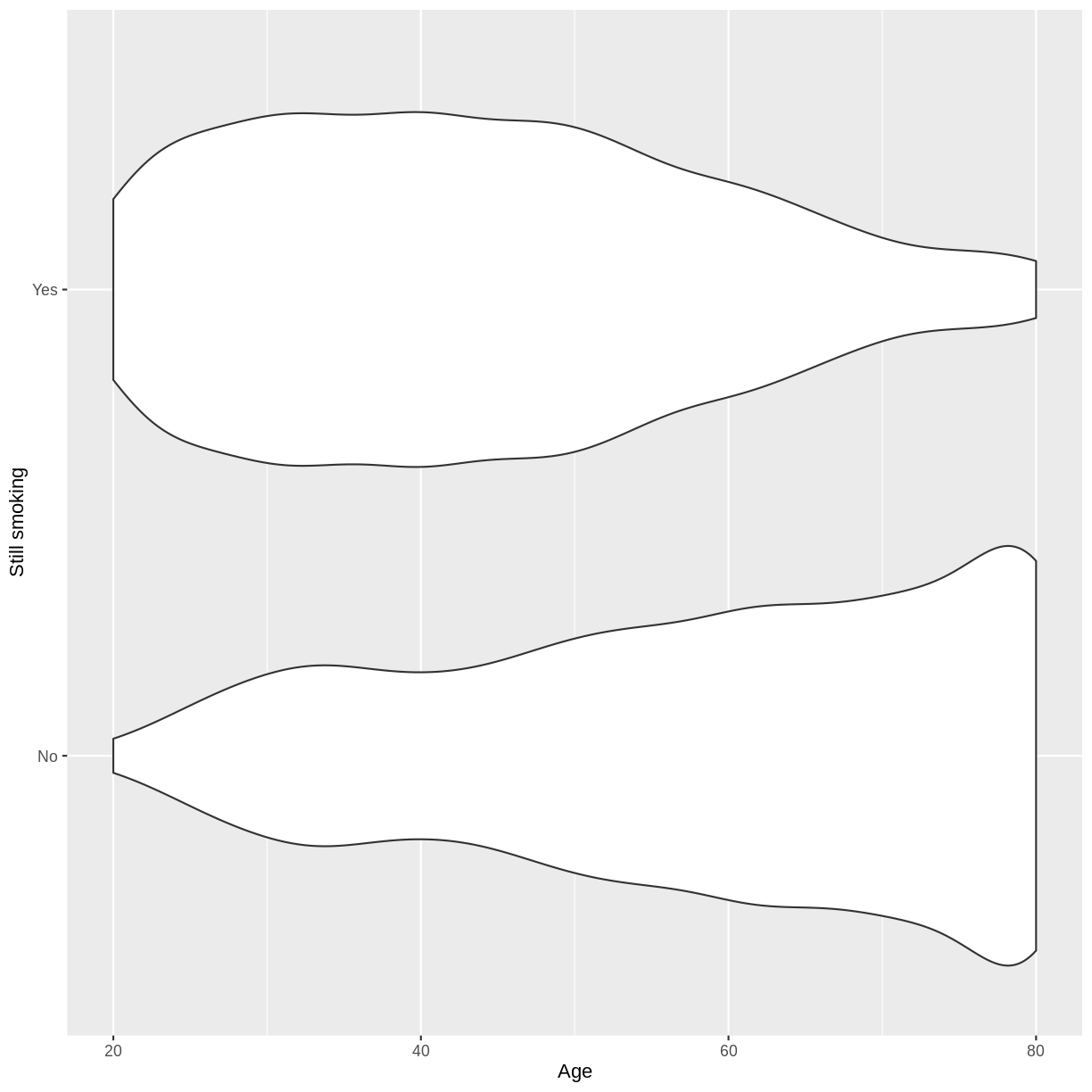
The plot suggests that on average, participants of younger age are still smoking and participants of older age have given up smoking. After the exercise, we can proceed with fitting the logistic regression model.
Exercise
You have been asked to model the relationship between physical activity (
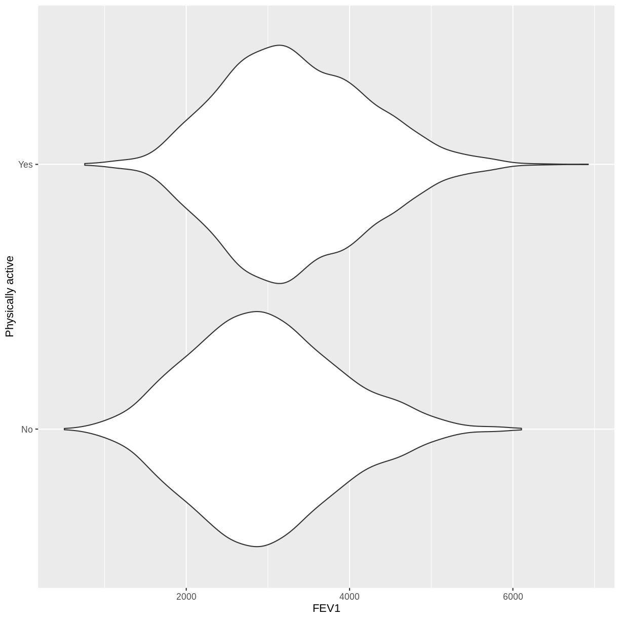
PhysActive) andFEV1in the NHANES data. Use theggplot2package to create an exploratory plot, ensuring that:
- NAs are discarded from the
PhysActivevariable.- Physical activity (
PhysActive) is on the y-axis and FEV1 (FEV1) on the x-axis.- These data are shown as a violin plot.
- The y-axis is labelled as “Physically active”.
Solution
dat %>%
  drop_na(PhysActive) %>%
  ggplot(aes(x = FEV1, y = PhysActive)) +
  geom_violin() +
  ylab("Physically active")
Fitting and interpreting the logistic regression model
We fit the model using glm(). As with the lm() command, we specify our response and explanatory variables with formula = SmokeNow ~ Age. In addition, we specify family = "binomial" so that a logistic regression model is fit by glm().
SmokeNow_Age <- dat %>%
  glm(formula = SmokeNow ~ Age, family = "binomial")
The logistic regression model equation associated with this model has the general form:
[\text{logit}(E(y)) = \beta_0 + \beta_1 \times x_1.]
Recall that $\beta_0$ estimates the log odds when $x_1 = 0$ and $\beta_1$ estimates the difference in the log odds associated with a one-unit difference in $x_1$. Using summ(), we can obtain estimates for $\beta_0$ and $\beta_1$:
summ(SmokeNow_Age, digits = 5)
MODEL INFO:
Observations: 3007 (6993 missing obs. deleted)
Dependent Variable: SmokeNow
Type: Generalized linear model
  Family: binomial
  Link function: logit

MODEL FIT:
χ²(1) = 574.29107, p = 0.00000
Pseudo-R² (Cragg-Uhler) = 0.23240
Pseudo-R² (McFadden) = 0.13853
AIC = 3575.26400, BIC = 3587.28139

Standard errors: MLE
------------------------------------------------------------
                        Est.      S.E.      z val.         p
----------------- ---------- --------- ----------- ---------
(Intercept)          2.60651   0.13242    19.68364   0.00000
Age                 -0.05423   0.00249   -21.77087   0.00000
------------------------------------------------------------
The equation therefore becomes:
[\text{logit}(E(\text{SmokeNow})) = 2.60651 - 0.05423 \times \text{Age}.]
Alternatively, we can express the model equation in terms of the probability of “success”:
[\text{Pr}(y = 1) = \text{logit}^{-1}(\beta_0 + \beta_1 \times x_1).]
In this example, $\text{SmokeNow} = \text{Yes}$ is “success”. The equation therefore becomes:
[\text{Pr}(\text{SmokeNow} = \text{Yes}) = \text{logit}^{-1}(2.60651 - 0.05423 \times \text{Age}).]
Recall that the odds of success,
$\frac{\text{Pr}(\text{SmokeNow} = \text{Yes})}{\text{Pr}(\text{SmokeNow} = \text{No})}$,
is multiplied by a factor of $e^{\beta_1}$ for every one-unit increase in $x_1$.
We can find this factor using summ(), including exp = TRUE:
summ(SmokeNow_Age, digits = 5, exp = TRUE)
MODEL INFO:
Observations: 3007 (6993 missing obs. deleted)
Dependent Variable: SmokeNow
Type: Generalized linear model
  Family: binomial
  Link function: logit

MODEL FIT:
χ²(1) = 574.29107, p = 0.00000
Pseudo-R² (Cragg-Uhler) = 0.23240
Pseudo-R² (McFadden) = 0.13853
AIC = 3575.26400, BIC = 3587.28139

Standard errors: MLE
-------------------------------------------------------------------------
                    exp(Est.)       2.5%      97.5%      z val.         p
----------------- ----------- ---------- ---------- ----------- ---------
(Intercept)          13.55161   10.45382   17.56738    19.68364   0.00000
Age                   0.94721    0.94260    0.95185   -21.77087   0.00000
-------------------------------------------------------------------------
The model therefore predicts that the odds of success will be multiplied by $0.94721$ for every one-unit increase in $x_1$.
Exercise
- Using the
glm()command, fit a logistic regression model of physical activity (PhysActive) as a function of FEV1 (FEV1). Name thisglmobjectPhysActive_FEV1.- Using the
summfunction from thejtoolspackage, answer the following questions:A) What log odds of physical activity does the model predict, on average, for an individual with an
FEV1of 0?
B) By how much is the log odds of physical activity expected to differ, on average, for a one-unit difference inFEV1?
C) Given these values and the names of the response and explanatory variables, how can the general equation $\text{logit}(E(y)) = \beta_0 + \beta_1 \times x_1$ be adapted to represent the model?
D) By how much is $\frac{\text{Pr}(\text{PhysActive} = \text{Yes})}{\text{Pr}(\text{PhysActive} = \text{No})}$ expected to be multiplied for a one-unit increase inFEV1?Solution
To answer questions A-C, we look at the default output from
summ():PhysActive_FEV1 <- dat %>% drop_na(PhysActive) %>% glm(formula = PhysActive ~ FEV1, family = "binomial") summ(PhysActive_FEV1, digits = 5)MODEL INFO: Observations: 5767 (1541 missing obs. deleted) Dependent Variable: PhysActive Type: Generalized linear model Family: binomial Link function: logit MODEL FIT: χ²(1) = 235.33619, p = 0.00000 Pseudo-R² (Cragg-Uhler) = 0.05364 Pseudo-R² (McFadden) = 0.02982 AIC = 7660.03782, BIC = 7673.35764 Standard errors: MLE ------------------------------------------------------------ Est. S.E. z val. p ----------------- ---------- --------- ----------- --------- (Intercept) -1.18602 0.10068 -11.78013 0.00000 FEV1 0.00046 0.00003 14.86836 0.00000 ------------------------------------------------------------A) -1.18602
B) The log odds of physical activity is expected to be 0.00046 for every unit increase inFEV1.
C) $\text{logit}(E(\text{PhysActive})) = -1.18602 + 0.00046 \times \text{FEV1}$.To answer question D, we add
exp = TRUEto thesumm()command:summ(PhysActive_FEV1, digits = 5, exp = TRUE)MODEL INFO: Observations: 5767 (1541 missing obs. deleted) Dependent Variable: PhysActive Type: Generalized linear model Family: binomial Link function: logit MODEL FIT: χ²(1) = 235.33619, p = 0.00000 Pseudo-R² (Cragg-Uhler) = 0.05364 Pseudo-R² (McFadden) = 0.02982 AIC = 7660.03782, BIC = 7673.35764 Standard errors: MLE ----------------------------------------------------------------------- exp(Est.) 2.5% 97.5% z val. p ----------------- ----------- --------- --------- ----------- --------- (Intercept) 0.30543 0.25074 0.37206 -11.78013 0.00000 FEV1 1.00046 1.00040 1.00052 14.86836 0.00000 -----------------------------------------------------------------------D) The multiplicative change in the odds of physical activity being “Yes” is estimated to be 1.00046.
Visualising the logistic regression model
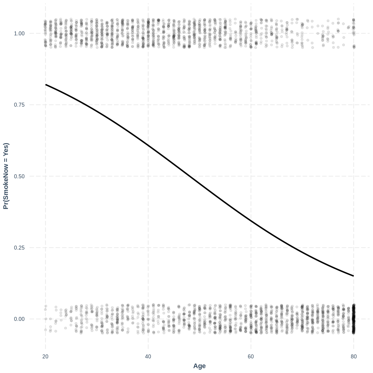
Finally, we can visualise our model using the effect_plot() function from the jtools
package. Importantly, logistic regression models are often visualised in terms of
the probability of success, i.e. $\text{Pr}(\text{SmokeNow} = \text{Yes})$ in our example.
We specify our model inside effect_plot(), alongside our explanatory variable of interest
with pred = Age. To aid interpretation of the model, we include the original data points
with plot.points = TRUE. Recall that our data is binary, so the data points are exclusively
$0$s and $1$s. To avoid overlapping points becoming hard to interpret, we add jitter using
jitter = c(0.1, 0.05) and opacity using point.alpha = 0.1.
We also change the y-axis label to “Pr(SmokeNow = Yes)” using ylab().
effect_plot(SmokeNow_Age, pred = Age, plot.points = TRUE,
            jitter = c(0.1, 0.05), point.alpha = 0.1) +
  ylab("Pr(SmokeNow = Yes)")
Exercise
To help others interpret the
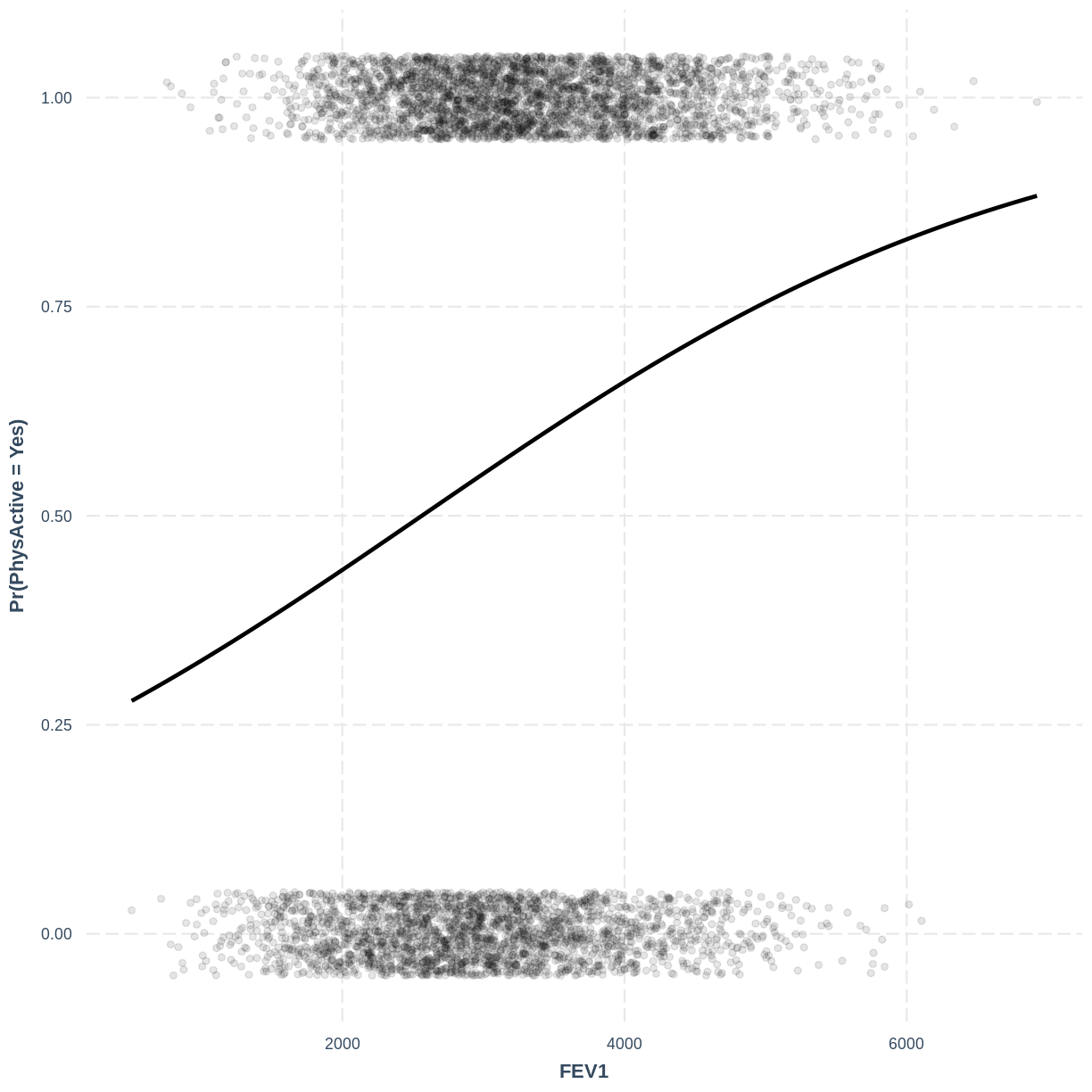
PhysActive_FEV1model, produce a figure. Make this figure using thejtoolspackage, ensuring that the y-axis is labelled as “Pr(PhysActive = Yes)”.Solution
effect_plot(PhysActive_FEV1, pred = FEV1, plot.points = TRUE,
            jitter = c(0.1, 0.05), point.alpha = 0.1) +
  ylab("Pr(PhysActive = Yes)")
Changing the direction of coding in the outcome variable
In this episode, the outcome variable
SmokeNowwas modelled with “Yes” as “success” and “No” as failure. The “success” and “failure” designations are arbitrary and merely convey the baseline and alternative levels for our model. In other words, “No” is taken as the baseline level and “Yes” is taken as the alternative level. As a result, our coefficients relate to the probability of individuals still smoking. Recall that this direction results from R taking the levels in alphabetical order.If we wanted to, we could change the direction of coding. As a result, our model coefficients would relate to the probability of no longer smoking.
We do this using
mutateandrelevel. Insiderelevel, we specify the new baseline level usingref = "Yes". We then fit the model as before:SmokeNow_Age_Relevel <- dat %>% mutate(SmokeNow = relevel(SmokeNow, ref = "Yes")) %>% glm(formula = SmokeNow ~ Age, family = "binomial")Looking at the output from
summ(), we see that the coefficients have changed:summ(SmokeNow_Age_Relevel, digits = 5)MODEL INFO: Observations: 3007 (6993 missing obs. deleted) Dependent Variable: SmokeNow Type: Generalized linear model Family: binomial Link function: logit MODEL FIT: χ²(1) = 574.29107, p = 0.00000 Pseudo-R² (Cragg-Uhler) = 0.23240 Pseudo-R² (McFadden) = 0.13853 AIC = 3575.26400, BIC = 3587.28139 Standard errors: MLE ------------------------------------------------------------ Est. S.E. z val. p ----------------- ---------- --------- ----------- --------- (Intercept) -2.60651 0.13242 -19.68364 0.00000 Age 0.05423 0.00249 21.77087 0.00000 ------------------------------------------------------------The model equation therefor becomes:
\[\text{logit}(E(\text{SmokeNow})) = -2.60651 + 0.05423 \times \text{Age}.\]Expressing the model in terms of the probability of success:
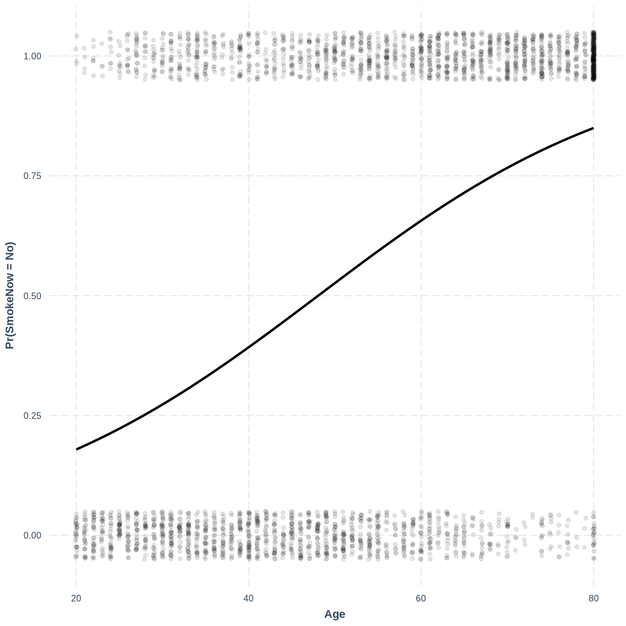
\[\text{Pr}(\text{SmokeNow} = \text{No}) = \text{logit}^{-1}(-2.60651 + 0.05423 \times \text{Age}).\]And finally creating the effect plot:
effect_plot(SmokeNow_Age_Relevel, pred = Age, plot.points = TRUE,
            jitter = c(0.1, 0.05), point.alpha = 0.1) +
  ylab("Pr(SmokeNow = No)")
Key Points
A violin plot can be used to explore the relationship between a binary response variable and a continuous explanatory variable.
Instead of
lm(),glm()withfamily = binomialis used to fit a logistic regression model.The default
summ()output shows the model coefficients in terms of the log odds.Adding
exp = TRUEtosumm()allows us to interpret the model in terms of the multiplicative change in the odds of success.The logistic regression model is visualised in terms of the probability of success.
Making predictions from a logistic regression model
Overview
Teaching: 20 min
Exercises: 20 minQuestions
How can we calculate predictions from a logistic regression model manually?
How can we calculate predictions from a logistic regression model in R?
Objectives
Calculate predictions in terms of the log odds, the odds and the probability of success from a logistic regression model using parameter estimates given by the model output.
Use the
make_predictions()function from thejtoolspackage to generate predictions from a logistic regression model in terms of the log odds, the odds and the probability of success.
As with the linear regression models, the logistic regression model allows us to make predictions. First we will calculate predictions of the log odds, the odds and the probability of success using the model equations. Then we will see how R can calculate predictions for us using the make_predictions() function.
Calculating predictions manually
Let us use the SmokeNow_Age model from the previous episode. The equation for this model in terms of the log odds was:
[\text{logit}(E(\text{SmokeNow})) = 2.60651 − 0.05423 \times \text{Age}.]
Therefore, for a 30-year old individual, the model predicts a log odds of
[\text{logit}(E(\text{SmokeNow})) = 2.60651 − 0.05423 \times 30 = 0.97961.]
Since the odds are more interpretable than the log odds, we can convert our log odds prediction to the odds scale. We do so by exponentiation the log odds:
[\frac{E(\text{SmokeNow})}{1-E(\text{SmokeNow})} = e^{0.97961} = 2.663.]
Therefore, the model predicts that individuals that have been smokers, are 2.663 as likely to still be smokers at the age of 30 than not.
Recall that the model could also be expressed in terms of the probability of “success”:
[\text{Pr}(\text{SmokeNow} = \text{Yes}) = \text{logit}^{-1}(2.60651 − 0.05423 \times \text{Age}).]
In R, we can calculate the inverse logit using the inv.logit() function from the boot package. Therefore, for a 30-year old individual, the model predicts a probability of $\text{SmokeNow} = \text{Yes}$:
inv.logit(2.60651 - 0.05423 * 30)
[1] 0.7270308
Or in mathematical notation: $\text{Pr}(\text{SmokeNow} = \text{Yes}) = \text{logit}^{-1}(2.60651 − 0.05423 \times 30) = 0.727.$
Exercise
Given the
summoutput from ourPhysActive_FEV1model, the model can be described as \(\text{logit}(E(\text{PhysActive})) = -1.18602 + 0.00046 \times \text{FEV1}.\)
A) Calculate the log odds of physical activity predicted by the model for an individual with an FEV1 of 3000.
B) Calculate the odds of physical activity predicted by the model for an individual with an FEV1 of 3000. How many more times is the individual likely to be physically active than not?
C) Using theinv.logit()function from the packageboot, calculate the probability of an individual with an FEV1 of 3000 being physically active.Solution
A) $\text{logit}(E(\text{PhysActive}) = -1.18602 + 0.00046 \times 3000 = 0.194.$
B) $e^{0.194} = 1.21$, so the individual is 1.21 times more likely to be physically active than not. This can be calculated in R as follows:exp(0.194)[1] 1.214096C) $\text{Pr}(\text{PhysActive}) = {logit}^{-1}(-1.18602 + 0.00046 \times 3000) = 0.548.$ This can be calculated in R as follows:
inv.logit(-1.18602 + 0.00046 * 3000)[1] 0.5483435
Calculating predictions using make_predictions()
Using the make_predictions() function brings two advantages. First, when calculating multiple predictions, we are saved the effort of inserting multiple values into our model manually and doing the calculations. Secondly, make_predictions() returns 95% confidence intervals around the predictions, giving us a sense of the uncertainty around the predictions.
To use make_predictions(), we need to create a tibble with the explanatory variable values for which we wish to have mean predictions from the model. We do this using the tibble() function. Note that the column name must correspond to the name of the explanatory variable in the model, i.e. Age. In the code below, we create a tibble with the values 30, 50 and 70. We then provide make_predictions() with this tibble, alongside the model from which we wish to have predictions.
Recall that we can calculate predictions on the log odds or the probability scale. To obtain predictions on the log odds scale, we include outcome.scale = "link" in our make_predictions() command. For example:
predictionDat <- tibble(Age = c(30, 50, 70)) #data for which we wish to predict

make_predictions(SmokeNow_Age, new_data = predictionDat,
                 outcome.scale = "link")
# A tibble: 3 × 4
    Age SmokeNow    ymax   ymin
  <dbl>    <dbl>   <dbl>  <dbl>
1    30    0.980  1.11    0.851
2    50   -0.105 -0.0257 -0.184
3    70   -1.19  -1.07   -1.31
From the output we can see that the model predicts a log odds of -0.105 for a 50-year old individual. The 95% confidence interval around this prediction is [-0.184, -0.0257].
To calculate predictions on the probability scale, we include outcome.scale = "response" in our make_predictions() command:
make_predictions(SmokeNow_Age, new_data = predictionDat,
                 outcome.scale = "response")
# A tibble: 3 × 4
    Age SmokeNow  ymax  ymin
  <dbl>    <dbl> <dbl> <dbl>
1    30    0.727 0.752 0.701
2    50    0.474 0.494 0.454
3    70    0.233 0.256 0.212
From the output we can see that the model predicts a probability of still smoking of 0.474 for a 50-year old individual. The 95% confidence interval around this prediction is [0.454, 0.494].
Exercise
Using the
make_predictions()function and thePhysActive_FEV1model:
A) Obtain the log odds of the expectation of physical activity for individuals with an FEV1 of 2000, 3000 or 4000. Ensure that your predictions include confidence intervals.
B) Exponentiate the log odds at an FEV1 of 4000. How many more times is an individual likely to be physically active than not with an FEV1 of 4000?
C) Obtain the probabilities of individuals with an FEV1 of 2000, 3000 or 4000 being physically active. Ensure that your predictions include confidence intervals.Solution
A) Including
outcome.scale = "link"gives us predictions on the log odds scale:predictionDat <- tibble(FEV1 = c(2000, 3000, 4000)) make_predictions(PhysActive_FEV1, new_data = predictionDat, outcome.scale = "link")# A tibble: 3 × 4 FEV1 PhysActive ymax ymin <dbl> <dbl> <dbl> <dbl> 1 2000 -0.261 -0.175 -0.347 2 3000 0.202 0.255 0.148 3 4000 0.664 0.740 0.589B) $e^{0.664} = 1.94$, so an individual is 1.94 times more likely to be physically active.
C) Includingoutcome.scale = "response"gives us predictions on the probability scale:make_predictions(PhysActive_FEV1, new_data = predictionDat, outcome.scale = "response")# A tibble: 3 × 4 FEV1 PhysActive ymax ymin <dbl> <dbl> <dbl> <dbl> 1 2000 0.435 0.456 0.414 2 3000 0.550 0.563 0.537 3 4000 0.660 0.677 0.643
Key Points
Predictions of the log odds, the odds and the probability of success can be manually calculated using the model’s equation.
Predictions of the log odds, the odds and the probability of success alongside 95% CIs can be obtained using the
make_predictions()function.
Assessing logistic regression fit and assumptions
Overview
Teaching: 50 min
Exercises: 25 minQuestions
How can we interpret McFadden’s $R^2$ and binned residual plots?
What are the assumptions of logistic regression?
Objectives
Interpret McFadden’s $R^2$ and binned residual plots as assessments of model fit.
Assess whether the assumptions of the logistic regression model have been violated.
In this episode we will check the fit and assumptions of logistic regression models. We will use a pseudo-$R^2$ measure of model fit. Most importantly, we will assess model fit visually using binned residual plots. Finally, we will touch upon the four logistic regression assumptions.
McFadden’s $R^2$ as a measure of model fit
$R^2$ and $R^2_{adj}$ are popular measures of model fit in linear regresssion. These metrics can take on values from 0 to 1, with higher values indicating that more of the outcome variation is accounted for by the dependent variables. However, these measures cannot be used in logistic regression. A wide variety of pseudo-$R^2$ metrics have been developed. We will use McFadden’s $R^2$ in this episode.
McFadden’s $R^2$ gives us an idea of the relative performance of our model
compared to a model that predicts the mean. Similarly to the original $R^2$,
McFadden’s $R^2$ ranges from 0 to 1, with higher values indicating better
relative performance. However, by the design of this metric, values close
to 1 are unlikely with real-world data. Therefore, a McFadden’s $R^2$ of 0.2
can already indicate a good relative performance. This metric is returned
by summ() from the jtools package.
As with the original $R^2$, this metric should not be used on its own to assess model fit. We will look at McFadden’s $R^2$ alongside binned residual plots in the next section.
Assessing model fit by plotting binned residuals
As with linear regression, residuals for logistic regression can be defined as the difference between observed values and values predicted by the model.
Plotting raw residual plots is not very insightful. For example,
let’s create residual plots for our SmokeNow_Age model. First, we
store the residuals, fitted values and explanatory variable in
a tibble named residualData.
Notice that inside resid(), we specify type = response. Also note
that fitted() returns fitted values on the probability scale.
Next, we create plotting objects p1 and p2, which will contain
residuals vs. fitted and residuals vs. Age, respectively.
We plot these together in one region using + from the patchwork package.
residualData <- tibble(resid = resid(SmokeNow_Age, type = "response"),
fitted = fitted(SmokeNow_Age),
age = SmokeNow_Age$model$Age)
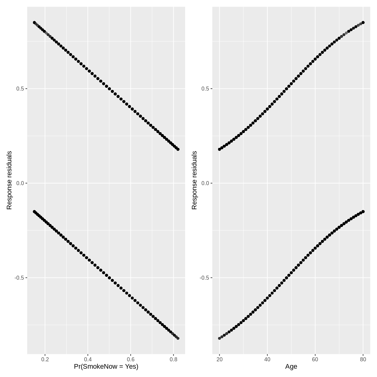
p1 <- ggplot(residualData, aes(x = fitted, y = resid)) +
geom_point(alpha = 0.3) +
xlab("Pr(SmokeNow = Yes)") +
ylab("Response residuals")
p2 <- ggplot(residualData, aes(x = age, y = resid)) +
geom_point(alpha = 0.3) +
xlab("Age") +
ylab("Response residuals")
p1 + p2
Let’s plot binned residuals instead. Binned residuals are averages of the residuals
plotted above, grouped by their associated fitted values or values for Age.
Binned residual plots can be made with the binnedplot from the arm package.
Rather than loading the arm package with library(), we specify the package
and function in one go using arm::binnedplot(). This prevents clashes between
arm and packages which we have loaded earlier in the lesson. Unfortunately,
binnedplot() does not work with patchwork. To create side-by-side plots,
we will use the command par(mfrow = c(1,2)) ahead of our plots.
Inside binnedplot(), we specify the x and y axes, as well as x and y axis labels.
We specify main = "" to suppress the default plot titles.
par(mfrow = c(1,2))

arm::binnedplot(x = residualData$fitted,
                y = residualData$resid,
                xlab = "Pr(SmokeNow = Yes)",
                ylab = "Average response residuals",
                main = "")

arm::binnedplot(x = residualData$age,
                y = residualData$resid,
                xlab = "Age",
                ylab = "Average response residuals",
                main = "")
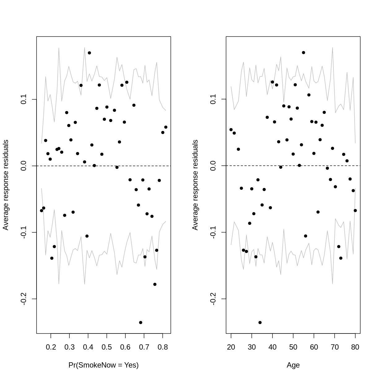
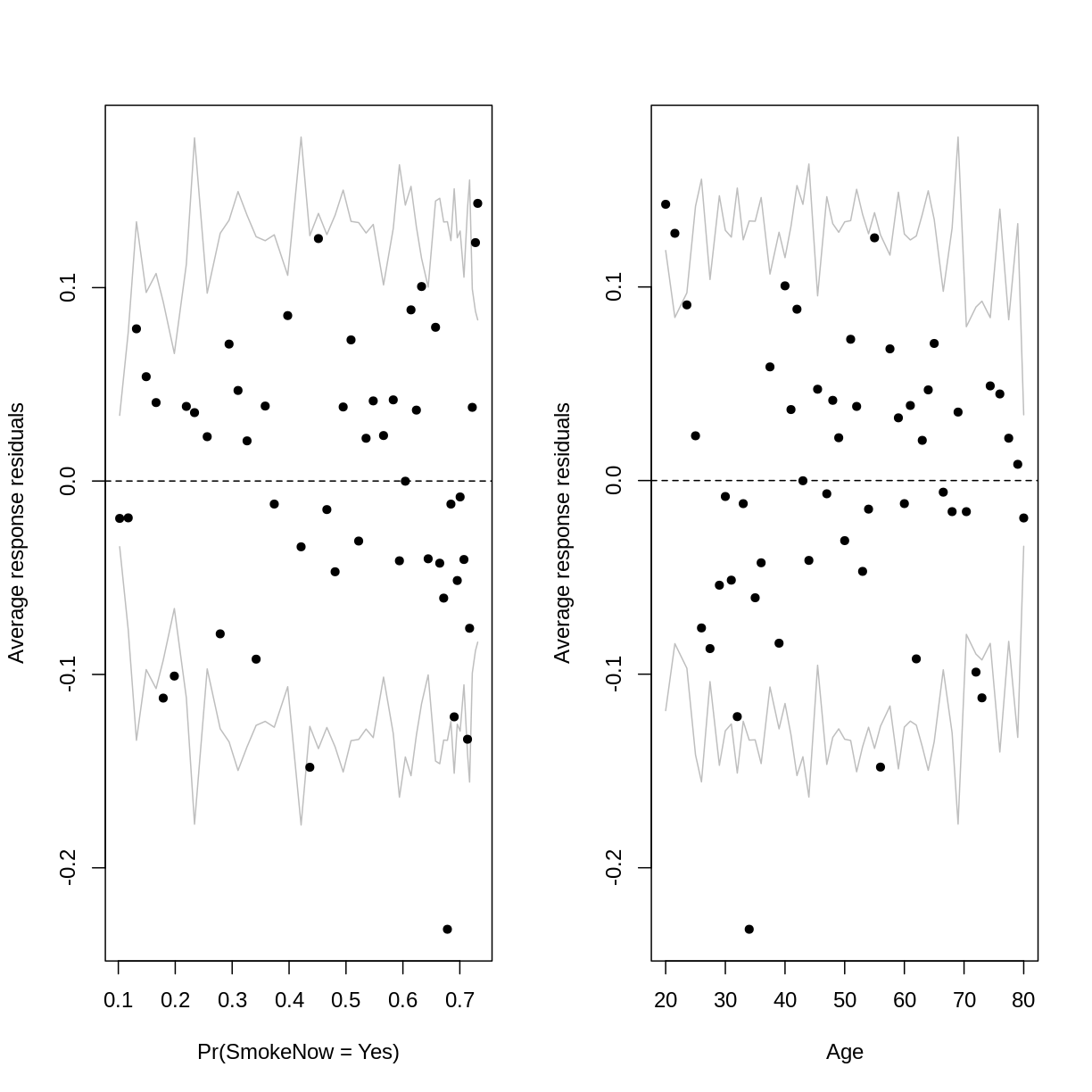
The outer lines on the plot indicate the bounds within which the binned residuals would be expected to fall, if the model provided a good fit to the data. There are three things to notice in these plots:
- For relatively low and high probabilities of success, the average binned residuals are more negative than would be expected with a good fit. The same goes for some lower and higher values of
Age. - For some probabilities towards the centre of the plot, as well as for some ages towards the centre of the plot, the residuals are more positive than would be expected with a good fit.
- The residuals appear to have a parabolic pattern.
Recall that a parabolic pattern can sometimes be resolved by squaring an
explanatory variable. Squaring Age indeed reduces the parabolic pattern:
SmokeNow_Age_SQ <- dat %>%
  glm(formula = SmokeNow ~ Age + I(Age^2),  family = "binomial")

residualData <- tibble(resid = resid(SmokeNow_Age_SQ, type = "response"),
                       fitted = fitted(SmokeNow_Age_SQ),
                       age = SmokeNow_Age_SQ$model$Age)

par(mfrow = c(1,2))

arm::binnedplot(x = residualData$fitted,
                y = residualData$resid,
                xlab = "Pr(SmokeNow = Yes)",
                ylab = "Average response residuals",
                main = "")

arm::binnedplot(x = residualData$age,
                y = residualData$resid,
                xlab = "Age",
                ylab = "Average response residuals",
                main = "")
Notice that we are still left with some average binned residuals, lying outside the lines, which suggest poor fit.
This may be unsurprising, as smoking habits are likely influenced by a lot more than Age alone.
At this point, we can also take a look at McFadden’s $R^2$ in the output from summ(). This comes
at 0.14, which is in line with the moderate fit suggested by the binned residuals.
summ(SmokeNow_Age_SQ)
MODEL INFO:
Observations: 3007 (6993 missing obs. deleted)
Dependent Variable: SmokeNow
Type: Generalized linear model
  Family: binomial
  Link function: logit

MODEL FIT:
χ²(2) = 598.83, p = 0.00
Pseudo-R² (Cragg-Uhler) = 0.24
Pseudo-R² (McFadden) = 0.14
AIC = 3552.72, BIC = 3570.75

Standard errors: MLE
------------------------------------------------
                     Est.   S.E.   z val.      p
----------------- ------- ------ -------- ------
(Intercept)          0.87   0.37     2.37   0.02
Age                  0.02   0.02     1.40   0.16
I(Age^2)            -0.00   0.00    -4.92   0.00
------------------------------------------------
Exercise
Create a binned residual plot for our
PhysActive_FEV1model. Then answer the following questions:
A) Where along the predicted probabilities does our model tend to overestimate or underestimate the probability of success compared to the original data?
B) What pattern do the residuals appear to follow?
C) Apply a transformation to resolve the pattern in the residuals. Then, create a new binned residuals plot to show that the pattern has been reduced.
D) What is McFadden’s $R^2$ for this new model? What does it suggest?Solution
A) Our model overestimates the probability of physical activity in two of the bins below the 0.4 probability. Our model underestimates the probability of physical activity in two of the bins around the probabilities of 0.5 and 0.65. See the binned residual plot below:
PhysActive_FEV1 <- dat %>%
 drop_na(PhysActive) %>%
 glm(formula = PhysActive ~ FEV1, family = "binomial")

arm::binnedplot(x = PhysActive_FEV1$fitted.values,
           y = resid(PhysActive_FEV1, type = "response"),
           xlab = "Pr(PhysActive = Yes)")
B) There appears to be a parabolic pattern to the residuals.
C) Adding a squaredFEV1term resolves most of the parabolic pattern:PhysActive_FEV1_SQ <- dat %>% drop_na(PhysActive) %>% glm(formula = PhysActive ~ FEV1 + I(FEV1^2), family = "binomial") arm::binnedplot(x = PhysActive_FEV1_SQ$fitted.values, y = resid(PhysActive_FEV1_SQ, type = "response"), xlab = "Pr(PhysActive = Yes)")
D) Since McFadden’s $R^2$ is 0.03, it suggests that FEV1 is not a strong predictor of physical activity.
summ(PhysActive_FEV1_SQ)MODEL INFO: Observations: 5767 (1541 missing obs. deleted) Dependent Variable: PhysActive Type: Generalized linear model Family: binomial Link function: logit MODEL FIT: χ²(2) = 253.69, p = 0.00 Pseudo-R² (Cragg-Uhler) = 0.06 Pseudo-R² (McFadden) = 0.03 AIC = 7643.69, BIC = 7663.67 Standard errors: MLE ------------------------------------------------ Est. S.E. z val. p ----------------- ------- ------ -------- ------ (Intercept) -2.27 0.27 -8.28 0.00 FEV1 0.00 0.00 6.93 0.00 I(FEV1^2) -0.00 0.00 -4.32 0.00 ------------------------------------------------
Assessing the assumptions of the logistic regression model
The assumptions underlying the logistic regression model are similar to those of the simple linear regression model. The key similarities and differences are:
- Validity, representativeness and independent errors are assessed in the same way. See this episode from the simple linear regression lesson for explanations and exercises for these assumptions.
- While logistic regression has the linearity and additivity assumption, it is slightly different. This assumption states that the logit of our outcome variable has a linear, additive relationship with the explanatory variables. Violations of the linearity assumption can sometimes be solved through transformation of explanatory variables. Violations of the additivity assumption can sometimes be solved through the inclusion of interactions.
- Homoscedasticity and normally distributed residuals are not assumptions underlying the logistic regression model.
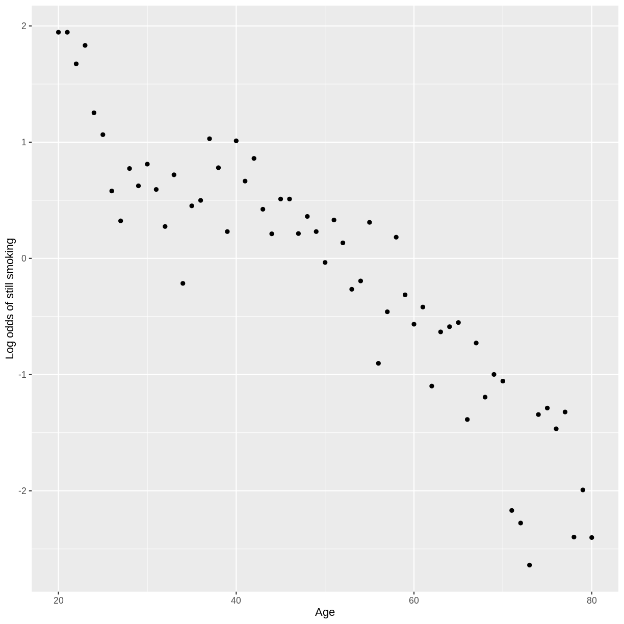
The linearity assumption can be checked as follows. Let’s take our
SmokeNow_Age model as an example. First, we drop NAs using drop_na().
Then, we group our observations by Age. This will allow us to calculate
the log odds for each value of Age. Then, we count the number of observations
in each level of SmokeNow across Age using count(). This allows us to calculate
the proportions using mutate(). We then filter for “success”, which is
SmokeNow == "Yes" in this case. We calculate the log odds using summarise().
Finally, we create a scatterplot of log odds versus Age. Broadly speaking,
the relationship looks fairly linear.
dat %>%
  drop_na(SmokeNow) %>%
  group_by(Age) %>%
  count(SmokeNow) %>%
  mutate(prop = n/sum(n)) %>%
  filter(SmokeNow == "Yes") %>%
  summarise(log_odds = log(prop/(1 - prop))) %>%
  ggplot(aes(x = Age, y = log_odds)) +
  geom_point() +
  ylab("Log odds of still smoking")
Key Points
McFadden’s $R^2$ measures relative performance, compared to a model that always predicts the mean. Binned residual plots allow us to check whether the residuals have a pattern and whether particular residuals are larger than expected, both indicating poor model fit.
The logistic regression assumptions are similar to the linear regression assumptions. However, linearity and additivity are checked with respect to the logit of the outcome variable. In addition, homoscedasticity and normality of residuals are not assumptions of binary logistic regression.