An introduction to binary response variables
Overview
Teaching: 40 min
Exercises: 20 minQuestions
How can we calculate probabilities of success and failure?
How do we interpret the expectation of a binary variable?
How can we calculate and interpret the odds?
How can we calculate and interpret the log odds?
Objectives
Calculate the probabilities of success and failure given binary data.
Interpret the expectation of a binary variable.
Calculate and interpret the odds of success given binary data.
Calculate and interpret the log odds of success given binary data.
In this lesson we will work with binary outcome variables. That is, variables which can take one of two possible values. For example, these could be $0$ or $1$, “success” or “failure” or “yes” or “no”.
Probabilities and expectation
By analysing binary data, we can estimate the probabilities of success and failure. For example, if we consider individuals between the ages of 55 and 66, we may be interested in the probability that individuals who have once smoked, are still smoking during the NHANES study.
The probability of success is estimated by the proportion of individuals who are still smoking. Similarly, the probability of failure is estimated by the proportion of individuals who are no longer smoking. In this context, we would consider an individual that still smokes a “success” and an individual that no longer smokes a “failure”.
We calculate these values in RStudio through four operations:
- Removing empty rows with
drop_na(); - Subsetting individuals of the appropriate age using
filter(); - Counting the number of individuals in each of the two levels of
SmokeNowusingcount(); - Calculating proportions by dividing the counts by the total number
of non-NA observations using
mutate().
dat %>%
  drop_na(SmokeNow) %>% # there are no empty rows in Age
                        # so we only use drop_na on SmokeNow
  filter(between(Age, 55, 66)) %>%
  count(SmokeNow, name = "n") %>%
  mutate(prop = n/sum(n))
  SmokeNow   n      prop
1       No 359 0.6232639
2      Yes 217 0.3767361
We see that the probability of success is estimated as $0.38$ and the probability
of failure is estimated as $0.62$. In mathematical notation:
$\text{Pr}(\text{SmokeNow} = \text{Yes}) = 0.38$ and $\text{Pr}(\text{SmokeNow} = \text{No}) = 0.62$.
You may have noticed that the probabilities of success and failure add to 1. This is true because there are only two possible outcomes for a binary response variable. Therefore, the probability of success equals 1 minus the probability of failure: $\text{Pr}(\text{Success}) = 1 - \text{Pr}(\text{Failure})$.
In the linear regression lessons, we modelled the expectation of the outcome variable, $E(y)$. In the case of binary variables, we will also work with the expectation of the outcome variable. When $y$ is a binary variable, $E(y)$ is equal to the probability of success. In our example above, $E(y) = \text{Pr}(\text{SmokeNow} = \text{Yes}) = 0.38$.
Exercise
You have been asked to study physical activity (
PhysActive) in individuals with an FEV1 (FEV1) between 3750 and 4250 in the NHANES data.
A) Estimate the probabilitites that someone is or is not physically active for individuals with an FEV1 between 3750 and 4250.
B) What value is $E(\text{PhysActive})$ for individuals with an FEV1 between 3750 and 4250?Solution
A) To obtain the probabilities:
dat %>%
  drop_na(PhysActive) %>%
  filter(between(FEV1, 3750, 4250)) %>%
  count(PhysActive) %>%
  mutate(prop = n/sum(n))
PhysActive n prop 1 No 242 0.3159269 2 Yes 524 0.6840731We therefore estimate the probability of physical activity to be $0.68$ and the probability of no physical activity to be $0.32$.
B) $E(\text{PhysActive}) = \text{Pr}(\text{PhysActive} = \text{Yes}) = 0.68$
Why does $E(y)$ equal the probability of success?
In general, the expectation of a variable equals its probability-weighted mean. This is calculated by taking the sum of all values that a variable can take on, each multiplied by the probability of that value occuring.
In mathematical notation, this is indicated by:
\[E(y) = \sum_i\Big(y_i \times \text{Pr}(y = y_i)\Big)\]In the case of a binary variable, the variable can take one of two values: $0$ and $1$. Therefore, the expectation becomes:
\[E(y) = \sum_i\Big(y_i \times \text{Pr}(y = y_i)\Big) = 0 \times \text{Pr}(y = 0) + 1 \times \text{Pr}(y = 1) = \text{Pr}(y = 1)\]Since “success” is considered $y=1$, the expectation of a binary variable equals the probability of success.
Odds and log odds
Besides probabilities, binary data is often interpreted through odds. The odds are defined as:
\[\frac{E(y)}{1-E(y)}.\]Since the expectation of $y$ equals the probability of success, the odds can also be written as:
\[\frac{E(y)}{1-E(y)} = \frac{\text{Pr}(\text{Success})}{1-\text{Pr}(\text{Success})} = \frac{\text{Pr}(\text{Success})}{\text{Pr}(\text{Failure})}.\]Therefore, an odds greater than $1$ indicates that the probability of success is greater than the probability of failure. For example, an odds of 1.5 indicates that success is 1.5 times as likely as failure. An odds less than $1$ indicates that the probability of failure is greater than the probability of success. For example, an odds of 0.75 indicates that success is 0.75 times as likely as failure.
Binary outcome variables can be modeled through the log odds. We can see the relationship between the log odds and the expectation in the plot below. As we can see in the plot, a log odds greater than zero is associated with a probability of success greater than 0.5. Likewise, a log odds smaller than 0 is associated with a probability of success less than 0.5.
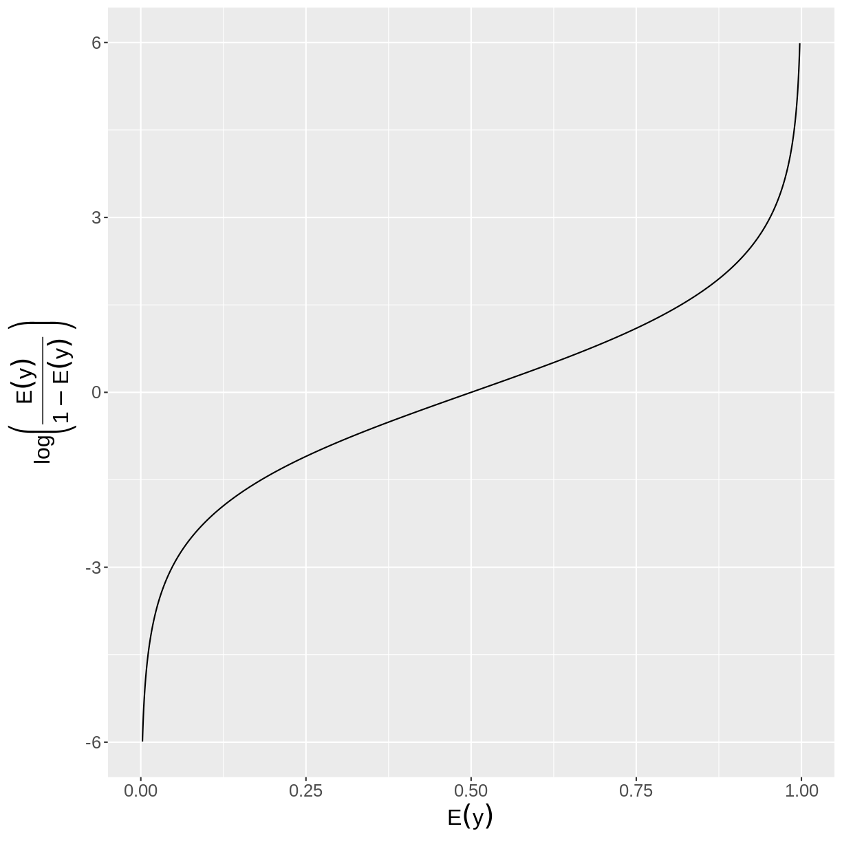
In mathematical notation, the log odds is defined as:
\[\text{log}\left(\frac{E(y)}{1-E(y)}\right).\]The interpretation of the probabilities, odds and log odds is summarised in the table below:
| Measure | Turning point | Interpretation |
|---|---|---|
| Probability | 0.5 | Proportion of observations that are successes |
| Odds | 1.0 | How many times more likely is success than failure? |
| Log odds | 0 | If log odds > 0, probability is > 0.5. |
The odds and the log odds can be calculated in RStudio through an
extension of the code that we used to calculate the probabilities.
From our table of probabilities we isolate the row with the probability
of success using filter(). We then calculate the odds and the log odds
using the summarise() function.
dat %>%
  drop_na(SmokeNow) %>%
  filter(between(Age, 55, 66)) %>%
  count(SmokeNow) %>%
  mutate(prop = n/sum(n)) %>%
  filter(SmokeNow == "Yes") %>%
  summarise(odds = prop/(1 - prop),
    log_odds = log(prop/(1 - prop)))
       odds  log_odds
1 0.6044568 -0.503425
Exercise
You have been asked to study physical activity (
PhysActive) in individuals with an FEV1 (FEV1) between 3750 and 4250 in the NHANES data. Calculate the odds and the log odds of physical activity for individuals with an FEV1 between 3750 and 4250. How is the odds interpreted here?Solution
dat %>%
  drop_na(PhysActive) %>%
  filter(between(FEV1, 3750, 4250)) %>%
  count(PhysActive) %>%
  mutate(prop = n/sum(n)) %>%
  filter(PhysActive == "Yes") %>%
  summarise(odds = prop/(1 - prop),
    log_odds = log(prop/(1 - prop)))
odds log_odds 1 2.165289 0.772554Since the odds equal 2.17, we expect individuals with an FEV1 between 3750 and 4250 to be 2.17 times more likely to be physically active than not.
What does $\text{log}()$ do?
The $\text{log}()$ is a transformation used widely in statistics, including in the modelling of binary variables. In general, $\text{log}_a(b)$ tells us to what power we need to raise $a$ to obtain the value $b$.
For example, $2^3 = 2 \times 2 \times 2 = 8$. Therefore, $\text{log}_2(8)=3$, since we raise $2$ to the power of $3$ to obtain 8.
Similarly, $\text{log}_3(81)=4$, since $3^4=81$.
In logistic regression, we use $\text{log}_{e}()$, where $e$ is a mathematical constant. The constant $e$ approximately equals 2.718.
Rather than writing $\text{log}_{e}()$, we write $\text{log}()$ for simplicity.
In R, we can calculate the log using the
log()function. For example, to calculate to what power we need to raise $e$ to obtain $10$:log(10)[1] 2.302585
Key Points
The probabilities of success and failure are estimated as the proportions of participants with a success and failure, respectively.
The expectation of a binary variable equals the probability of success.
The odds equal the ratio of the probability of success and one minus the probability of success. The odds quantify how many times more likely success is than failure.
The log odds are calculated by taking the log of the odds. When the log odds are greater than 0, the probability of success is greater than 0.5.