Assessing logistic regression fit and assumptions

Overview

Teaching: 50 min
Exercises: 25 min

Questions

• How can we interpret McFadden’s $R^2$ and binned residual plots?

• What are the assumptions of logistic regression?

Objectives

• Interpret McFadden’s $R^2$ and binned residual plots as assessments of model fit.

• Assess whether the assumptions of the logistic regression model have been violated.

In this episode we will check the fit and assumptions of logistic regression models. We will use a pseudo-$R^2$ measure of model fit. Most importantly, we will assess model fit visually using binned residual plots. Finally, we will touch upon the four logistic regression assumptions.

McFadden’s $R^2$ as a measure of model fit

$R^2$ and $R^2_{adj}$ are popular measures of model fit in linear regresssion. These metrics can take on values from 0 to 1, with higher values indicating that more of the outcome variation is accounted for by the dependent variables. However, these measures cannot be used in logistic regression. A wide variety of pseudo-$R^2$ metrics have been developed. We will use McFadden’s $R^2$ in this episode.

McFadden’s $R^2$ gives us an idea of the relative performance of our model compared to a model that predicts the mean. Similarly to the original $R^2$, McFadden’s $R^2$ ranges from 0 to 1, with higher values indicating better relative performance. However, by the design of this metric, values close to 1 are unlikely with real-world data. Therefore, a McFadden’s $R^2$ of 0.2 can already indicate a good relative performance. This metric is returned by summ() from the jtools package.

As with the original $R^2$, this metric should not be used on its own to assess model fit. We will look at McFadden’s $R^2$ alongside binned residual plots in the next section.

Assessing model fit by plotting binned residuals

As with linear regression, residuals for logistic regression can be defined as the difference between observed values and values predicted by the model.

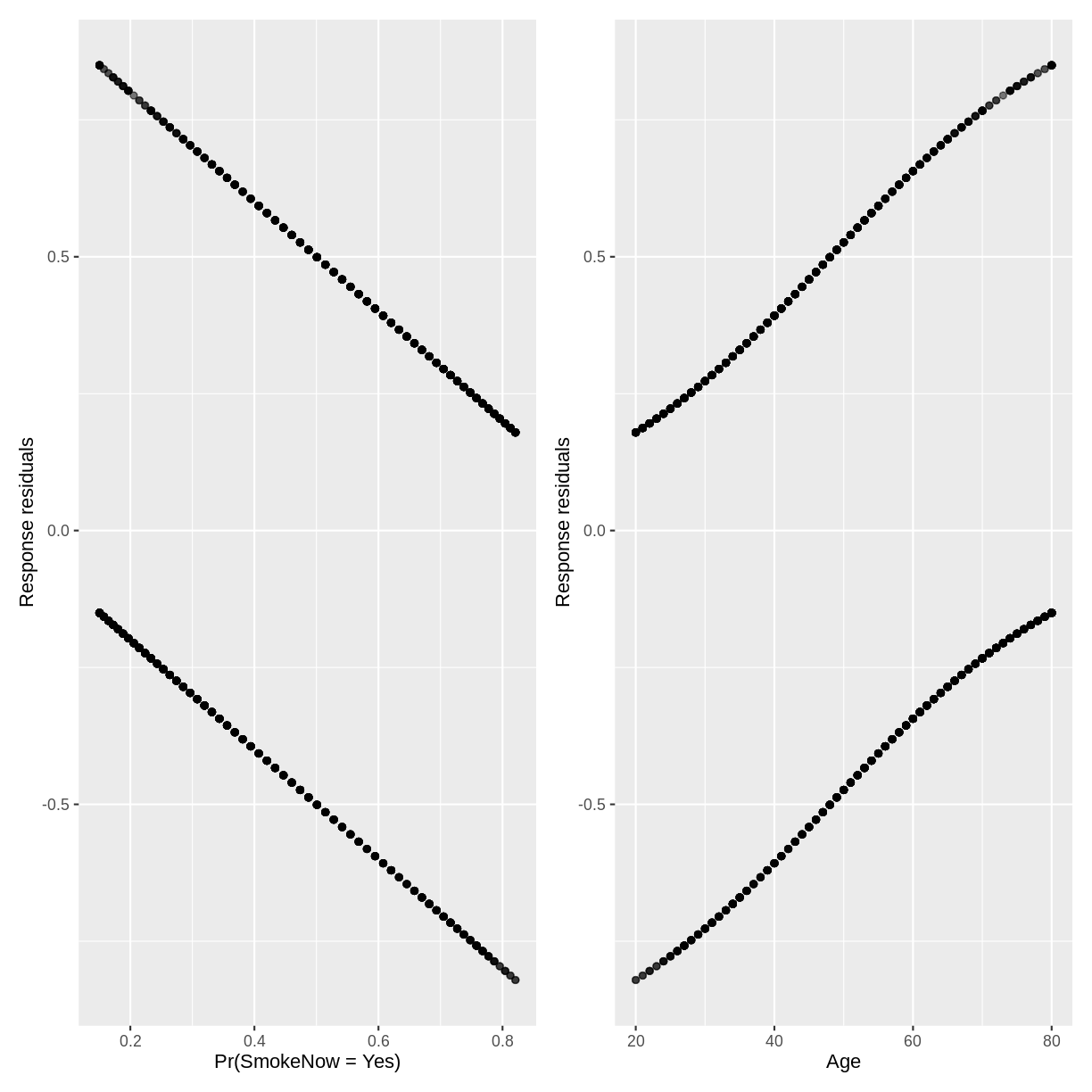
Plotting raw residual plots is not very insightful. For example, let’s create residual plots for our SmokeNow_Age model. First, we store the residuals, fitted values and explanatory variable in a tibble named residualData. Notice that inside resid(), we specify type = response. Also note that fitted() returns fitted values on the probability scale. Next, we create plotting objects p1 and p2, which will contain residuals vs. fitted and residuals vs. Age, respectively. We plot these together in one region using + from the patchwork package.

residualData <- tibble(resid = resid(SmokeNow_Age, type = "response"),
                       fitted = fitted(SmokeNow_Age),
                       age = SmokeNow_Age$model$Age)

p1 <- ggplot(residualData, aes(x = fitted, y = resid)) +
  geom_point(alpha = 0.3) +
  xlab("Pr(SmokeNow = Yes)") +
  ylab("Response residuals")

p2 <- ggplot(residualData, aes(x = age, y = resid)) +
 geom_point(alpha = 0.3) +
  xlab("Age") +
  ylab("Response residuals")

p1 + p2

Let’s plot binned residuals instead. Binned residuals are averages of the residuals plotted above, grouped by their associated fitted values or values for Age. Binned residual plots can be made with the binnedplot from the arm package. Rather than loading the arm package with library(), we specify the package and function in one go using arm::binnedplot(). This prevents clashes between arm and packages which we have loaded earlier in the lesson. Unfortunately, binnedplot() does not work with patchwork. To create side-by-side plots, we will use the command par(mfrow = c(1,2)) ahead of our plots.

Inside binnedplot(), we specify the x and y axes, as well as x and y axis labels. We specify main = "" to suppress the default plot titles.

par(mfrow = c(1,2))

arm::binnedplot(x = residualData$fitted,
                y = residualData$resid,
                xlab = "Pr(SmokeNow = Yes)",
                ylab = "Average response residuals",
                main = "") 

arm::binnedplot(x = residualData$age,
                y = residualData$resid,
                xlab = "Age",
                ylab = "Average response residuals",
                main = "")

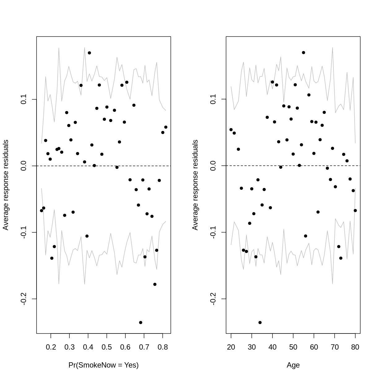
The outer lines on the plot indicate the bounds within which the binned residuals would be expected to fall, if the model provided a good fit to the data. There are three things to notice in these plots:

• For relatively low and high probabilities of success, the average binned residuals are more negative than would be expected with a good fit. The same goes for some lower and higher values of Age.
• For some probabilities towards the centre of the plot, as well as for some ages towards the centre of the plot, the residuals are more positive than would be expected with a good fit.
• The residuals appear to have a parabolic pattern.

Recall that a parabolic pattern can sometimes be resolved by squaring an explanatory variable. Squaring Age indeed reduces the parabolic pattern:

SmokeNow_Age_SQ <- dat %>%
  glm(formula = SmokeNow ~ Age + I(Age^2),  family = "binomial")

residualData <- tibble(resid = resid(SmokeNow_Age_SQ, type = "response"),
                       fitted = fitted(SmokeNow_Age_SQ),
                       age = SmokeNow_Age_SQ$model$Age)

par(mfrow = c(1,2))

arm::binnedplot(x = residualData$fitted,
                y = residualData$resid,
                xlab = "Pr(SmokeNow = Yes)",
                ylab = "Average response residuals",
                main = "") 

arm::binnedplot(x = residualData$age,
                y = residualData$resid,
                xlab = "Age",
                ylab = "Average response residuals",
                main = "")

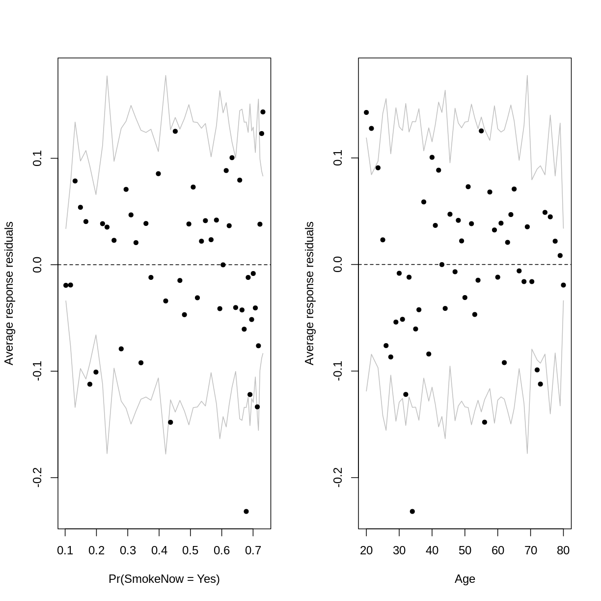
Notice that we are still left with some average binned residuals, lying outside the lines, which suggest poor fit. This may be unsurprising, as smoking habits are likely influenced by a lot more than Age alone.

At this point, we can also take a look at McFadden’s $R^2$ in the output from summ(). This comes at 0.14, which is in line with the moderate fit suggested by the binned residuals.

summ(SmokeNow_Age_SQ)

MODEL INFO:
Observations: 3007 (6993 missing obs. deleted)
Dependent Variable: SmokeNow
Type: Generalized linear model
  Family: binomial 
  Link function: logit 

MODEL FIT:
χ²(2) = 598.83, p = 0.00
Pseudo-R² (Cragg-Uhler) = 0.24
Pseudo-R² (McFadden) = 0.14
AIC = 3552.72, BIC = 3570.75 

Standard errors: MLE
------------------------------------------------
                     Est.   S.E.   z val.      p
----------------- ------- ------ -------- ------
(Intercept)          0.87   0.37     2.37   0.02
Age                  0.02   0.02     1.40   0.16
I(Age^2)            -0.00   0.00    -4.92   0.00
------------------------------------------------

Exercise

Create a binned residual plot for our PhysActive_FEV1 model. Then answer the following questions:
A) Where along the predicted probabilities does our model tend to overestimate or underestimate the probability of success compared to the original data?
B) What pattern do the residuals appear to follow?
C) Apply a transformation to resolve the pattern in the residuals. Then, create a new binned residuals plot to show that the pattern has been reduced.
D) What is McFadden’s $R^2$ for this new model? What does it suggest?

Solution

A) Our model overestimates the probability of physical activity in two of the bins below the 0.4 probability. Our model underestimates the probability of physical activity in two of the bins around the probabilities of 0.5 and 0.65. See the binned residual plot below:

PhysActive_FEV1 <- dat %>%
 drop_na(PhysActive) %>%
 glm(formula = PhysActive ~ FEV1, family = "binomial")

arm::binnedplot(x = PhysActive_FEV1$fitted.values,
           y = resid(PhysActive_FEV1, type = "response"),
           xlab = "Pr(PhysActive = Yes)") 

B) There appears to be a parabolic pattern to the residuals.
C) Adding a squared FEV1 term resolves most of the parabolic pattern:

PhysActive_FEV1_SQ <- dat %>%
 drop_na(PhysActive) %>%
 glm(formula = PhysActive ~ FEV1 + I(FEV1^2), family = "binomial")

arm::binnedplot(x = PhysActive_FEV1_SQ$fitted.values,
           y = resid(PhysActive_FEV1_SQ, type = "response"),
           xlab = "Pr(PhysActive = Yes)") 

D) Since McFadden’s $R^2$ is 0.03, it suggests that FEV1 is not a strong predictor of physical activity.

summ(PhysActive_FEV1_SQ)

MODEL INFO:
Observations: 5767 (1541 missing obs. deleted)
Dependent Variable: PhysActive
Type: Generalized linear model
  Family: binomial 
  Link function: logit 

MODEL FIT:
χ²(2) = 253.69, p = 0.00
Pseudo-R² (Cragg-Uhler) = 0.06
Pseudo-R² (McFadden) = 0.03
AIC = 7643.69, BIC = 7663.67 

Standard errors: MLE
------------------------------------------------
                     Est.   S.E.   z val.      p
----------------- ------- ------ -------- ------
(Intercept)         -2.27   0.27    -8.28   0.00
FEV1                 0.00   0.00     6.93   0.00
I(FEV1^2)           -0.00   0.00    -4.32   0.00
------------------------------------------------

Assessing the assumptions of the logistic regression model

The assumptions underlying the logistic regression model are similar to those of the simple linear regression model. The key similarities and differences are:

• Validity, representativeness and independent errors are assessed in the same way. See this episode from the simple linear regression lesson for explanations and exercises for these assumptions.
• While logistic regression has the linearity and additivity assumption, it is slightly different. This assumption states that the logit of our outcome variable has a linear, additive relationship with the explanatory variables. Violations of the linearity assumption can sometimes be solved through transformation of explanatory variables. Violations of the additivity assumption can sometimes be solved through the inclusion of interactions.
• Homoscedasticity and normally distributed residuals are not assumptions underlying the logistic regression model.

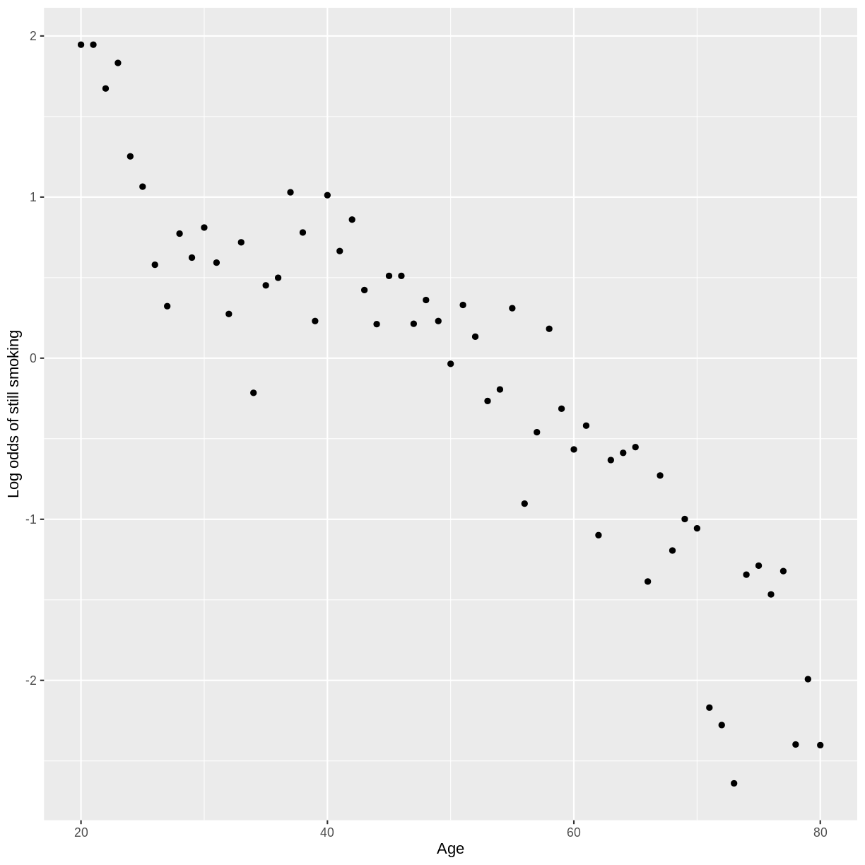
The linearity assumption can be checked as follows. Let’s take our SmokeNow_Age model as an example. First, we drop NAs using drop_na(). Then, we group our observations by Age. This will allow us to calculate the log odds for each value of Age. Then, we count the number of observations in each level of SmokeNow across Age using count(). This allows us to calculate the proportions using mutate(). We then filter for “success”, which is SmokeNow == "Yes" in this case. We calculate the log odds using summarise(). Finally, we create a scatterplot of log odds versus Age. Broadly speaking, the relationship looks fairly linear.

dat %>%
  drop_na(SmokeNow) %>%
  group_by(Age) %>%
  count(SmokeNow) %>%
  mutate(prop = n/sum(n)) %>%
  filter(SmokeNow == "Yes") %>%
  summarise(log_odds = log(prop/(1 - prop))) %>%
  ggplot(aes(x = Age, y = log_odds)) +
  geom_point() +
  ylab("Log odds of still smoking")

Key Points

• McFadden’s $R^2$ measures relative performance, compared to a model that always predicts the mean. Binned residual plots allow us to check whether the residuals have a pattern and whether particular residuals are larger than expected, both indicating poor model fit.

• The logistic regression assumptions are similar to the linear regression assumptions. However, linearity and additivity are checked with respect to the logit of the outcome variable. In addition, homoscedasticity and normality of residuals are not assumptions of binary logistic regression.