Logistic regression with one continuous explanatory variable

Overview

Teaching: 25 min
Exercises: 25 min

Questions

• How can we visualise the relationship between a binary response variable and a continuous explanatory variable in R?

• How can we fit a logistic regression model in R?

• How can we interpret the output of a logistic regression model in terms of the log odds in R?

• How can we interpret the output of a logistic regression model in terms of the multiplicative change in the odds of success in R?

• How can we visualise a logistic regression model in R?

Objectives

• Use the ggplot2 package to explore the relationship between a binary response variable and a continuous explanatory variable.

• Use the glm() function to fit a logistic regression model with one continuous explanatory variable.

• Use the summ() function from the jtools package to interpret the model output in terms of the log odds.

• Use the summ() function from the jtools package to interpret the model output in terms of the multiplicative change in the odds of success.

• Use the jtools and ggplot2 packages to visualise the resulting model.

In this episode we will learn to fit a logistic regression model when we have one binary response variable and one continuous explanatory variable.

Exploring the relationship between the binary and continuous variables

Before we fit the model, we can explore the relationship between our variables graphically. We are getting a sense of whether, on average, observations split along the binary variable appear to differ in the explanatory variable.

Let us take response variable SmokeNow and the continuous explanatory variable Age as an example. For participants that have smoked at least 100 cigarettes in their life, SmokeNow denotes whether they still smoke. The code below drops NAs in the response variable. The plotting is then initiated using ggplot(). Inside aes(), we select the response variable with y = SmokeNow and the continuous explanatory variable with x = Age. Then, the violin plots are called using geom_violin(). Finally, we edit the y-axis label using ylab().

dat %>%
  drop_na(SmokeNow) %>%
  ggplot(aes(x = Age, y = SmokeNow)) +
  geom_violin() +
  ylab("Still smoking")

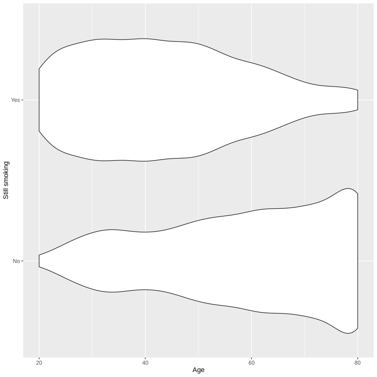
The plot suggests that on average, participants of younger age are still smoking and participants of older age have given up smoking. After the exercise, we can proceed with fitting the logistic regression model.

Exercise

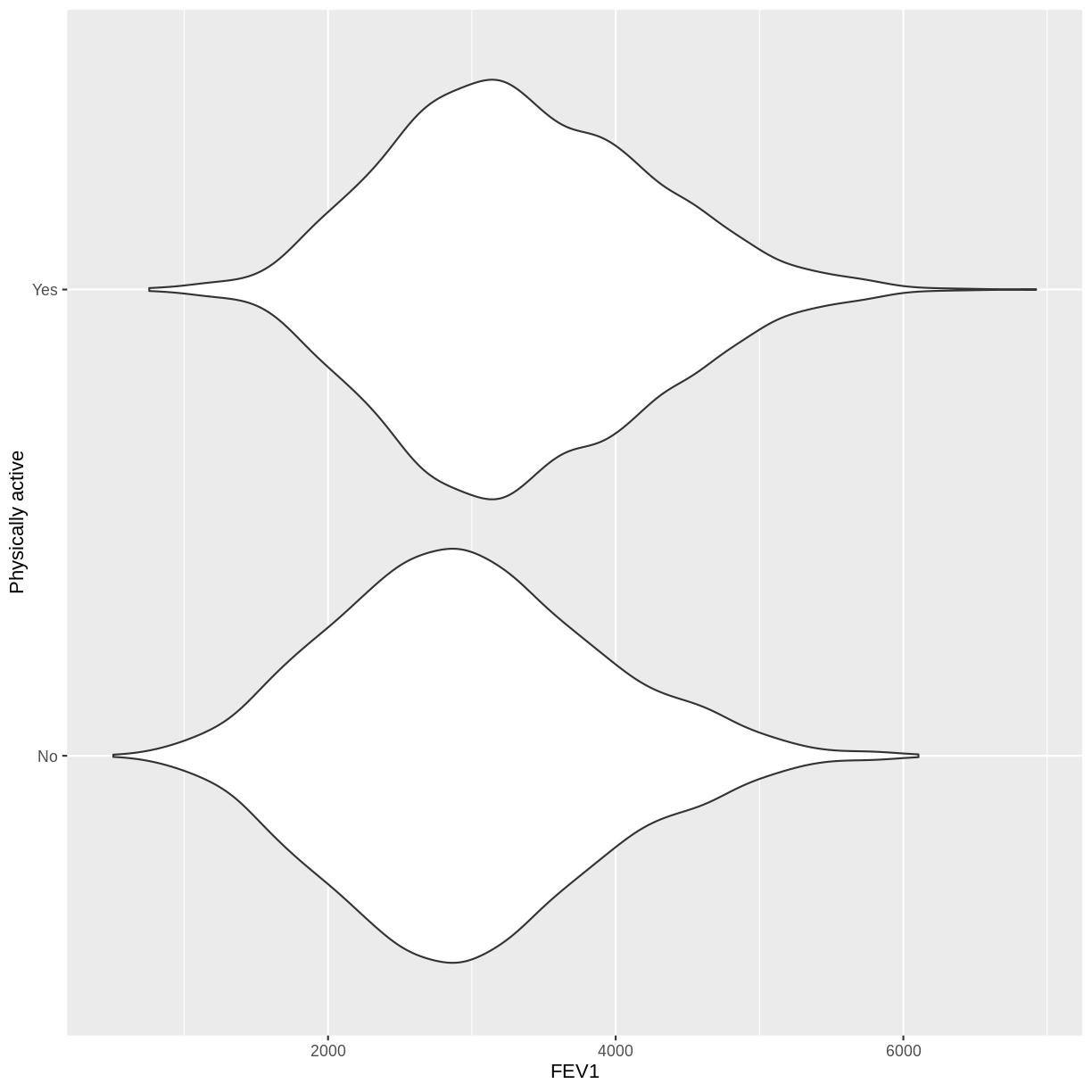
You have been asked to model the relationship between physical activity (PhysActive) and FEV1 in the NHANES data. Use the ggplot2 package to create an exploratory plot, ensuring that:

1. NAs are discarded from the PhysActive variable.
2. Physical activity (PhysActive) is on the y-axis and FEV1 (FEV1) on the x-axis.
3. These data are shown as a violin plot.
4. The y-axis is labelled as “Physically active”.

Solution

dat %>%
  drop_na(PhysActive) %>%
  ggplot(aes(x = FEV1, y = PhysActive)) +
  geom_violin() +
  ylab("Physically active")

Fitting and interpreting the logistic regression model

We fit the model using glm(). As with the lm() command, we specify our response and explanatory variables with formula = SmokeNow ~ Age. In addition, we specify family = "binomial" so that a logistic regression model is fit by glm().

SmokeNow_Age <- dat %>%
  glm(formula = SmokeNow ~ Age, family = "binomial")

The logistic regression model equation associated with this model has the general form:

Recall that $\beta_0$ estimates the log odds when $x_1 = 0$ and $\beta_1$ estimates the difference in the log odds associated with a one-unit difference in $x_1$. Using summ(), we can obtain estimates for $\beta_0$ and $\beta_1$:

summ(SmokeNow_Age, digits = 5)

MODEL INFO:
Observations: 3007 (6993 missing obs. deleted)
Dependent Variable: SmokeNow
Type: Generalized linear model
  Family: binomial 
  Link function: logit 

MODEL FIT:
χ²(1) = 574.29107, p = 0.00000
Pseudo-R² (Cragg-Uhler) = 0.23240
Pseudo-R² (McFadden) = 0.13853
AIC = 3575.26400, BIC = 3587.28139 

Standard errors: MLE
------------------------------------------------------------
                        Est.      S.E.      z val.         p
----------------- ---------- --------- ----------- ---------
(Intercept)          2.60651   0.13242    19.68364   0.00000
Age                 -0.05423   0.00249   -21.77087   0.00000
------------------------------------------------------------

The equation therefore becomes:

Alternatively, we can express the model equation in terms of the probability of “success”:

In this example, $\text{SmokeNow} = \text{Yes}$ is “success”. The equation therefore becomes:

Recall that the odds of success, $\frac{\text{Pr}(\text{SmokeNow} = \text{Yes})}{\text{Pr}(\text{SmokeNow} = \text{No})}$, is multiplied by a factor of $e^{\beta_1}$ for every one-unit increase in $x_1$. We can find this factor using summ(), including exp = TRUE:

summ(SmokeNow_Age, digits = 5, exp = TRUE)

MODEL INFO:
Observations: 3007 (6993 missing obs. deleted)
Dependent Variable: SmokeNow
Type: Generalized linear model
  Family: binomial 
  Link function: logit 

MODEL FIT:
χ²(1) = 574.29107, p = 0.00000
Pseudo-R² (Cragg-Uhler) = 0.23240
Pseudo-R² (McFadden) = 0.13853
AIC = 3575.26400, BIC = 3587.28139 

Standard errors: MLE
-------------------------------------------------------------------------
                    exp(Est.)       2.5%      97.5%      z val.         p
----------------- ----------- ---------- ---------- ----------- ---------
(Intercept)          13.55161   10.45382   17.56738    19.68364   0.00000
Age                   0.94721    0.94260    0.95185   -21.77087   0.00000
-------------------------------------------------------------------------

The model therefore predicts that the odds of success will be multiplied by $0.94721$ for every one-unit increase in $x_1$.

Exercise

1. Using the glm() command, fit a logistic regression model of physical activity (PhysActive) as a function of FEV1 (FEV1). Name this glm object PhysActive_FEV1.
2. Using the summ function from the jtools package, answer the following questions:

A) What log odds of physical activity does the model predict, on average, for an individual with an FEV1 of 0?
B) By how much is the log odds of physical activity expected to differ, on average, for a one-unit difference in FEV1?
C) Given these values and the names of the response and explanatory variables, how can the general equation $\text{logit}(E(y)) = \beta_0 + \beta_1 \times x_1$ be adapted to represent the model?
D) By how much is $\frac{\text{Pr}(\text{PhysActive} = \text{Yes})}{\text{Pr}(\text{PhysActive} = \text{No})}$ expected to be multiplied for a one-unit increase in FEV1?

Solution

To answer questions A-C, we look at the default output from summ():

PhysActive_FEV1 <- dat %>%
  drop_na(PhysActive) %>%
  glm(formula = PhysActive ~ FEV1, family = "binomial")

summ(PhysActive_FEV1, digits = 5)

MODEL INFO:
Observations: 5767 (1541 missing obs. deleted)
Dependent Variable: PhysActive
Type: Generalized linear model
  Family: binomial 
  Link function: logit 

MODEL FIT:
χ²(1) = 235.33619, p = 0.00000
Pseudo-R² (Cragg-Uhler) = 0.05364
Pseudo-R² (McFadden) = 0.02982
AIC = 7660.03782, BIC = 7673.35764 

Standard errors: MLE
------------------------------------------------------------
                        Est.      S.E.      z val.         p
----------------- ---------- --------- ----------- ---------
(Intercept)         -1.18602   0.10068   -11.78013   0.00000
FEV1                 0.00046   0.00003    14.86836   0.00000
------------------------------------------------------------

A) -1.18602
B) The log odds of physical activity is expected to be 0.00046 for every unit increase in FEV1.
C) $\text{logit}(E(\text{PhysActive})) = -1.18602 + 0.00046 \times \text{FEV1}$.

To answer question D, we add exp = TRUE to the summ() command:

summ(PhysActive_FEV1, digits = 5, exp = TRUE)

MODEL INFO:
Observations: 5767 (1541 missing obs. deleted)
Dependent Variable: PhysActive
Type: Generalized linear model
  Family: binomial 
  Link function: logit 

MODEL FIT:
χ²(1) = 235.33619, p = 0.00000
Pseudo-R² (Cragg-Uhler) = 0.05364
Pseudo-R² (McFadden) = 0.02982
AIC = 7660.03782, BIC = 7673.35764 

Standard errors: MLE
-----------------------------------------------------------------------
                    exp(Est.)      2.5%     97.5%      z val.         p
----------------- ----------- --------- --------- ----------- ---------
(Intercept)           0.30543   0.25074   0.37206   -11.78013   0.00000
FEV1                  1.00046   1.00040   1.00052    14.86836   0.00000
-----------------------------------------------------------------------

D) The multiplicative change in the odds of physical activity being “Yes” is estimated to be 1.00046.

Visualising the logistic regression model

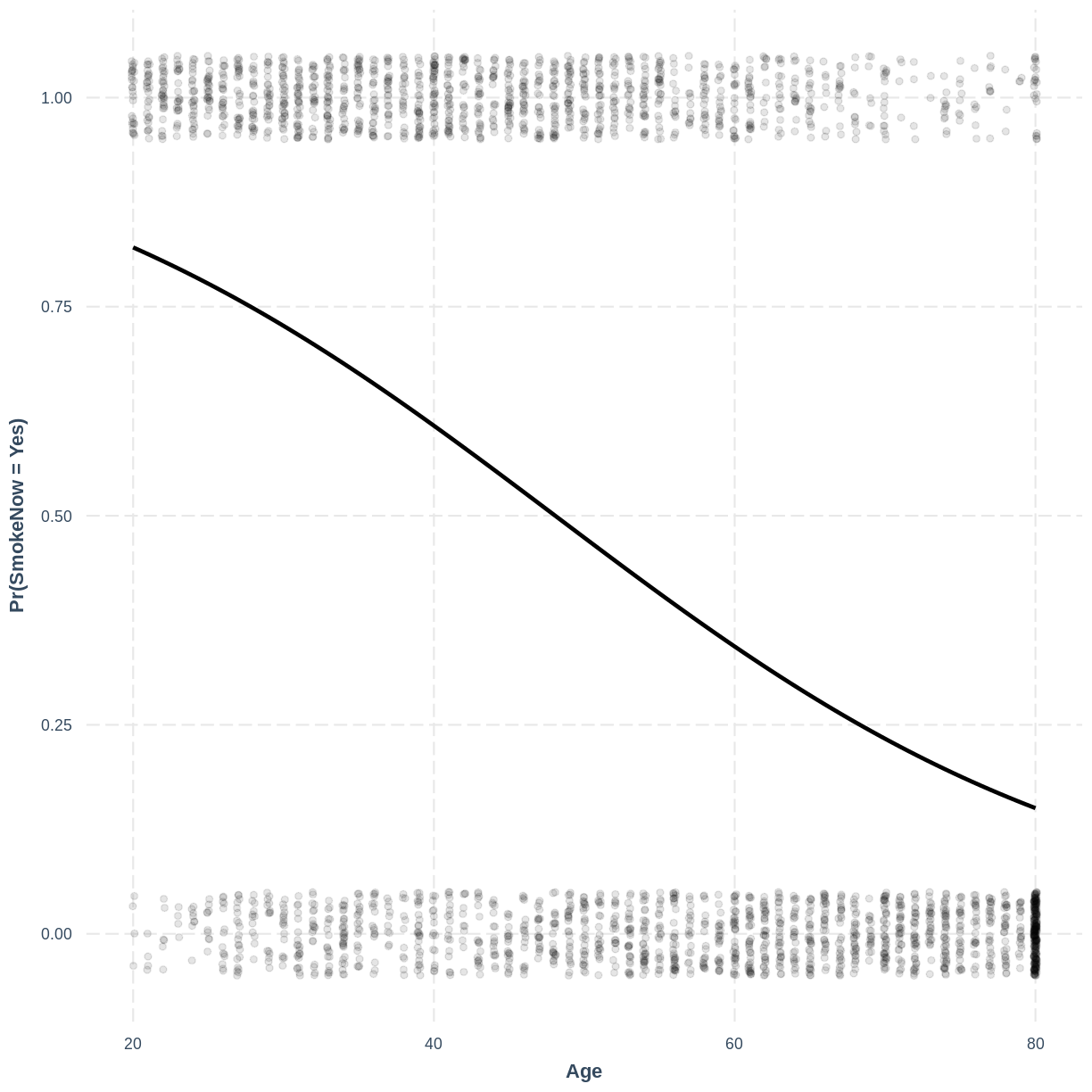
Finally, we can visualise our model using the effect_plot() function from the jtools package. Importantly, logistic regression models are often visualised in terms of the probability of success, i.e. $\text{Pr}(\text{SmokeNow} = \text{Yes})$ in our example.

We specify our model inside effect_plot(), alongside our explanatory variable of interest with pred = Age. To aid interpretation of the model, we include the original data points with plot.points = TRUE. Recall that our data is binary, so the data points are exclusively $0$s and $1$s. To avoid overlapping points becoming hard to interpret, we add jitter using jitter = c(0.1, 0.05) and opacity using point.alpha = 0.1. We also change the y-axis label to “Pr(SmokeNow = Yes)” using ylab().

effect_plot(SmokeNow_Age, pred = Age, plot.points = TRUE,
            jitter = c(0.1, 0.05), point.alpha = 0.1) +
  ylab("Pr(SmokeNow = Yes)")

Exercise

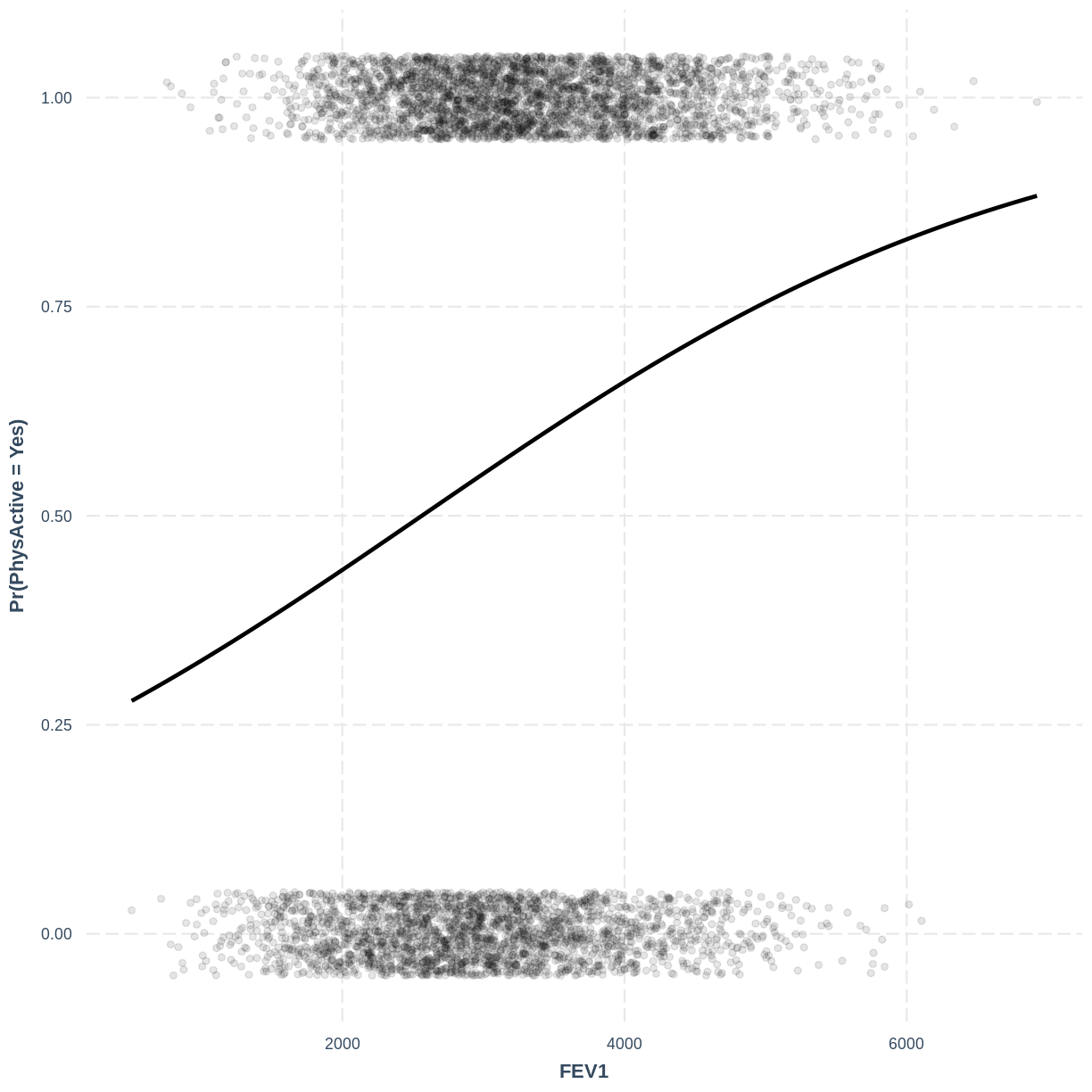
To help others interpret the PhysActive_FEV1 model, produce a figure. Make this figure using the jtools package, ensuring that the y-axis is labelled as “Pr(PhysActive = Yes)”.

Solution

effect_plot(PhysActive_FEV1, pred = FEV1, plot.points = TRUE,
            jitter = c(0.1, 0.05), point.alpha = 0.1) +
  ylab("Pr(PhysActive = Yes)")

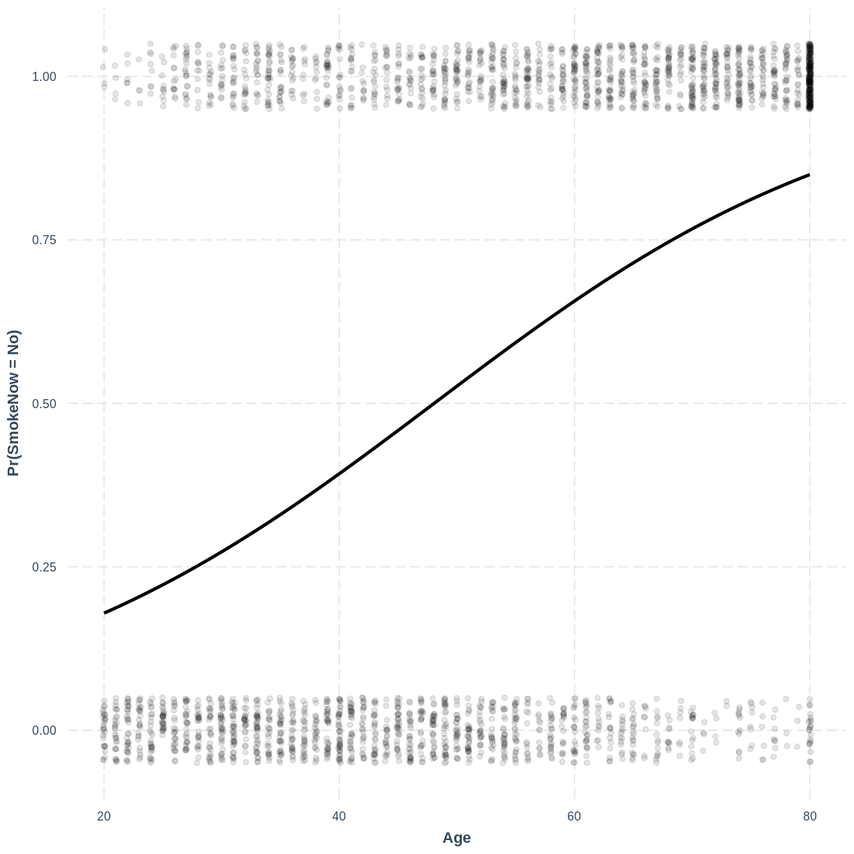
Changing the direction of coding in the outcome variable

In this episode, the outcome variable SmokeNow was modelled with “Yes” as “success” and “No” as failure. The “success” and “failure” designations are arbitrary and merely convey the baseline and alternative levels for our model. In other words, “No” is taken as the baseline level and “Yes” is taken as the alternative level. As a result, our coefficients relate to the probability of individuals still smoking. Recall that this direction results from R taking the levels in alphabetical order.

If we wanted to, we could change the direction of coding. As a result, our model coefficients would relate to the probability of no longer smoking.

We do this using mutate and relevel. Inside relevel, we specify the new baseline level using ref = "Yes". We then fit the model as before:

SmokeNow_Age_Relevel <- dat %>%
  mutate(SmokeNow = relevel(SmokeNow, ref = "Yes")) %>%
  glm(formula = SmokeNow ~ Age, family = "binomial")

Looking at the output from summ(), we see that the coefficients have changed:

summ(SmokeNow_Age_Relevel, digits = 5)

MODEL INFO:
Observations: 3007 (6993 missing obs. deleted)
Dependent Variable: SmokeNow
Type: Generalized linear model
  Family: binomial 
  Link function: logit 

MODEL FIT:
χ²(1) = 574.29107, p = 0.00000
Pseudo-R² (Cragg-Uhler) = 0.23240
Pseudo-R² (McFadden) = 0.13853
AIC = 3575.26400, BIC = 3587.28139 

Standard errors: MLE
------------------------------------------------------------
                        Est.      S.E.      z val.         p
----------------- ---------- --------- ----------- ---------
(Intercept)         -2.60651   0.13242   -19.68364   0.00000
Age                  0.05423   0.00249    21.77087   0.00000
------------------------------------------------------------

The model equation therefor becomes:

\[\text{logit}(E(\text{SmokeNow})) = -2.60651 + 0.05423 \times \text{Age}.\]

Expressing the model in terms of the probability of success:

\[\text{Pr}(\text{SmokeNow} = \text{No}) = \text{logit}^{-1}(-2.60651 + 0.05423 \times \text{Age}).\]

And finally creating the effect plot:

effect_plot(SmokeNow_Age_Relevel, pred = Age, plot.points = TRUE,
            jitter = c(0.1, 0.05), point.alpha = 0.1) +
  ylab("Pr(SmokeNow = No)")

Key Points

• A violin plot can be used to explore the relationship between a binary response variable and a continuous explanatory variable.

• Instead of lm(), glm() with family = binomial is used to fit a logistic regression model.

• The default summ() output shows the model coefficients in terms of the log odds.

• Adding exp = TRUE to summ() allows us to interpret the model in terms of the multiplicative change in the odds of success.

• The logistic regression model is visualised in terms of the probability of success.