Factor analysis
Last updated on 2026-04-22 | Edit this page
Overview
Questions
- What is factor analysis and when can it be used?
- What are communality and uniqueness in factor analysis?
- How to decide on the number of factors to use?
- How to interpret the output of factor analysis?
Objectives
- Perform a factor analysis on high-dimensional data.
- Select an appropriate number of factors.
- Interpret the output of factor analysis.
Introduction
Biologists often encounter high-dimensional datasets from which they wish to extract underlying features – they need to carry out dimensionality reduction. The last episode dealt with one method to achieve this, called principal component analysis (PCA), which expressed new dimension-reduced components as linear combinations of the original features in the dataset. Principal components can therefore be difficult to interpret. Here, we introduce a related but more interpretable method called factor analysis (FA), which constructs new components, called factors, that explicitly represent underlying (latent) constructs in our data. Like PCA, FA uses linear combinations, but uses latent constructs instead. FA is therefore often more interpretable and useful when we would like to extract meaning from our dimension-reduced set of variables.
There are two types of FA, called exploratory and confirmatory factor analysis (EFA and CFA). Both EFA and CFA aim to reproduce the observed relationships among a group of features with a smaller set of latent variables. EFA is used in a descriptive (exploratory) manner to uncover which measured variables are reasonable indicators of the various latent dimensions. In contrast, CFA is conducted in an a priori, hypothesis-testing manner that requires strong empirical or theoretical foundations. We will mainly focus on EFA here, which is used to group features into a specified number of latent factors.
Unlike with PCA, researchers using FA have to specify the number of latent variables (factors) at the point of running the analysis. Researchers may use exploratory data analysis methods (including PCA) to provide an initial estimate of how many factors adequately explain the variation observed in a dataset. In practice, a range of different values is usually tested.
Motivating example: student scores
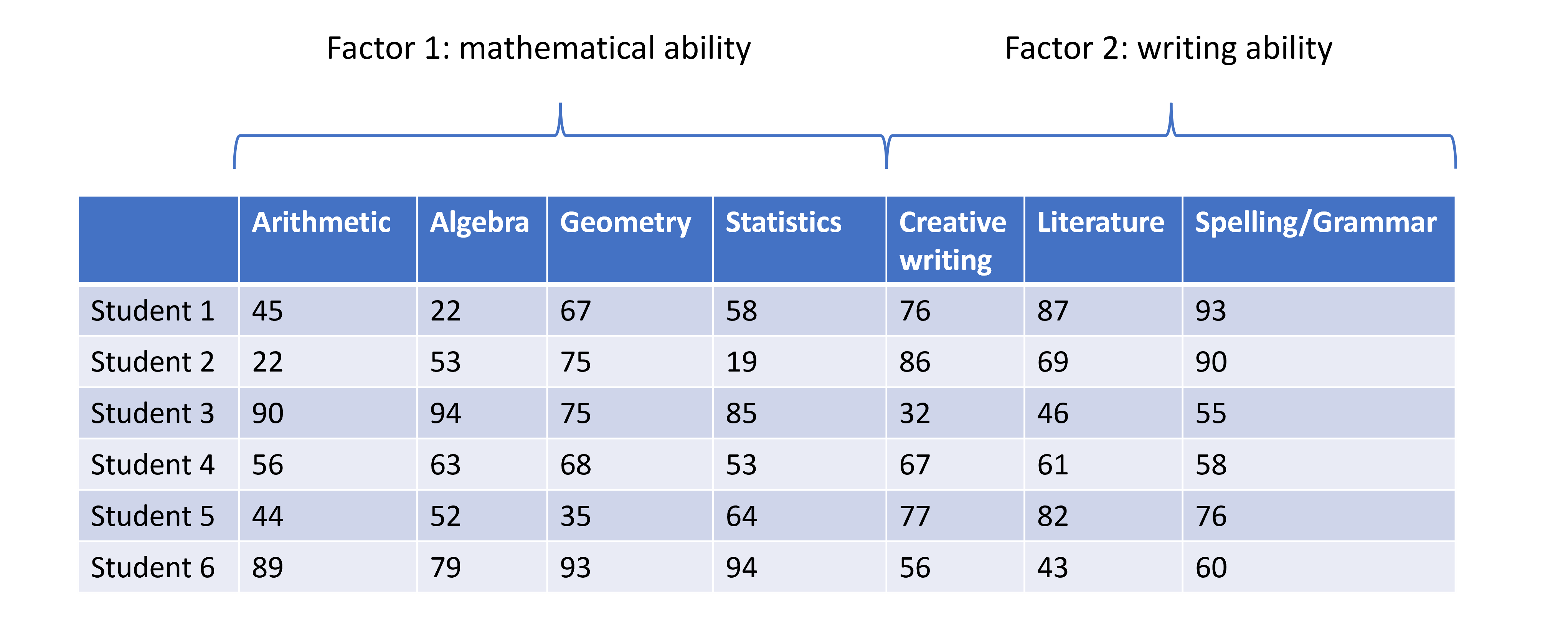
One scenario for using FA would be whether student scores in different subjects can be summarised by certain subject categories. Take a look at the hypothetical dataset below. If we were to run and EFA on this, we might find that the scores can be summarised well by two factors, which we can then interpret. We have labelled these hypothetical factors “mathematical ability” and “writing ability”.
So, EFA is designed to identify a specified number of unobservable factors from observable features contained in the original dataset. This is slightly different from PCA, which does not do this directly. Just to recap, PCA creates as many principal components as there are features in the dataset, each component representing a different linear combination of features. The principal components are ordered by the amount of variance they account for.
Prostate cancer patient data
We revisit the [prostate]((https://carpentries-incubator.github.io/high-dimensional-stats-r/data/index.html)
dataset of 97 men who have prostate cancer. Although not strictly a
high-dimensional dataset, as with other episodes, we use this dataset to
explore the method.
In this example, we use the clinical variables to identify factors representing various clinical variables from prostate cancer patients. Two principal components have already been identified as explaining a large proportion of variance in the data when these data were analysed in the PCA episode. We may expect a similar number of factors to exist in the data.
Let’s subset the data to just include the log-transformed clinical variables for the purposes of this episode:
R
prostate <- readRDS("data/prostate.rds")
R
nrow(prostate)
OUTPUT
[1] 97R
head(prostate)
OUTPUT
      lcavol  lweight age      lbph svi       lcp gleason pgg45       lpsa
1 -0.5798185 2.769459  50 -1.386294   0 -1.386294       6     0 -0.4307829
2 -0.9942523 3.319626  58 -1.386294   0 -1.386294       6     0 -0.1625189
3 -0.5108256 2.691243  74 -1.386294   0 -1.386294       7    20 -0.1625189
4 -1.2039728 3.282789  58 -1.386294   0 -1.386294       6     0 -0.1625189
5  0.7514161 3.432373  62 -1.386294   0 -1.386294       6     0  0.3715636
6 -1.0498221 3.228826  50 -1.386294   0 -1.386294       6     0  0.7654678
R
#select five log-transformed clinical variables for further analysis
pros2 <- prostate[, c("lcavol", "lweight", "lbph", "lcp", "lpsa")]
head(pros2)
OUTPUT
      lcavol  lweight      lbph       lcp       lpsa
1 -0.5798185 2.769459 -1.386294 -1.386294 -0.4307829
2 -0.9942523 3.319626 -1.386294 -1.386294 -0.1625189
3 -0.5108256 2.691243 -1.386294 -1.386294 -0.1625189
4 -1.2039728 3.282789 -1.386294 -1.386294 -0.1625189
5  0.7514161 3.432373 -1.386294 -1.386294  0.3715636
6 -1.0498221 3.228826 -1.386294 -1.386294  0.7654678
Performing exploratory factor analysis
EFA may be implemented in R using the factanal()
function from the stats package (which is
a built-in package in base R). This function fits a factor analysis by
maximising the log-likelihood using a data matrix as input. The number
of factors to be fitted in the analysis is specified by the user using
the factors argument.
Challenge 1 (3 mins)
Use the factanal() function to identify the minimum
number of factors necessary to explain most of the variation in the
data
R
# Include one factor only
pros_fa <- factanal(pros2, factors = 1)
pros_fa
OUTPUT
Call:
factanal(x = pros2, factors = 1)

Uniquenesses:
 lcavol lweight    lbph     lcp    lpsa
  0.149   0.936   0.994   0.485   0.362

Loadings:
        Factor1
lcavol  0.923
lweight 0.253
lbph
lcp     0.718
lpsa    0.799

               Factor1
SS loadings      2.074
Proportion Var   0.415

Test of the hypothesis that 1 factor is sufficient.
The chi square statistic is 29.81 on 5 degrees of freedom.
The p-value is 1.61e-05
R
# p-value <0.05 suggests that one factor is not sufficient
# we reject the null hypothesis that one factor captures full
# dimensionality in the dataset

# Include two factors
pros_fa <- factanal(pros2, factors = 2)
pros_fa
OUTPUT
Call:
factanal(x = pros2, factors = 2)

Uniquenesses:
 lcavol lweight    lbph     lcp    lpsa
  0.121   0.422   0.656   0.478   0.317

Loadings:
        Factor1 Factor2
lcavol   0.936
lweight  0.165   0.742
lbph             0.586
lcp      0.722
lpsa     0.768   0.307

               Factor1 Factor2
SS loadings      2.015   0.992
Proportion Var   0.403   0.198
Cumulative Var   0.403   0.601

Test of the hypothesis that 2 factors are sufficient.
The chi square statistic is 0.02 on 1 degree of freedom.
The p-value is 0.878
R
# p-value >0.05 suggests that two factors is sufficient
# we cannot reject the null hypothesis that two factors captures
# full dimensionality in the dataset

#Include three factors
pros_fa <- factanal(pros2, factors = 3)
ERROR
Error in `factanal()`:
! 3 factors are too many for 5 variables
R
# Error shows that fitting three factors are not appropriate
# for only 5 variables (number of factors too high)
The output of factanal() shows the loadings for each of
the input variables associated with each factor. The loadings are values
between -1 and 1 which represent the relative contribution each input
variable makes to the factors. Positive values show that these variables
are positively related to the factors, while negative values show a
negative relationship between variables and factors. Loading values are
missing for some variables because R does not print loadings less than
0.1.
How many factors do we need?
There are numerous ways to select the “best” number of factors. One
is to use the minimum number of features that does not leave a
significant amount of variance unaccounted for. In practice, we repeat
the factor analysis for different numbers of factors (by specifying
different values in the factors argument). If we have an
idea of how many factors there will be before analysis, we can start
with that number. The final section of the analysis output then shows
the results of a hypothesis test in which the null hypothesis is that
the number of factors used in the model is sufficient to capture most of
the variation in the dataset. If the p-value is less than our
significance level (for example 0.05), we reject the null hypothesis
that the number of factors is sufficient and we repeat the analysis with
more factors. When the p-value is greater than our significance level,
we do not reject the null hypothesis that the number of factors used
captures variation in the data. We may therefore conclude that this
number of factors is sufficient.
Like PCA, the fewer factors that can explain most of the variation in the dataset, the better. It is easier to explore and interpret results using a smaller number of factors which represent underlying features in the data.
Variance accounted for by factors - communality and uniqueness
The communality of a variable is the sum of its squared loadings. It represents the proportion of the variance in a variable that is accounted for by the FA model.
Uniqueness is the opposite of communality and represents the amount of variation in a variable that is not accounted for by the FA model. Uniqueness is calculated by subtracting the communality value from 1. If uniqueness is high for a given variable, that means this variable is not well explained/accounted for by the factors identified.
R
apply(pros_fa$loadings^2, 1, sum) #communality
OUTPUT
   lcavol   lweight      lbph       lcp      lpsa
0.8793780 0.5782317 0.3438669 0.5223639 0.6832788
R
1 - apply(pros_fa$loadings^2, 1, sum) #uniqueness
OUTPUT
   lcavol   lweight      lbph       lcp      lpsa
0.1206220 0.4217683 0.6561331 0.4776361 0.3167212
Visualising the contribution of each variable to the factors
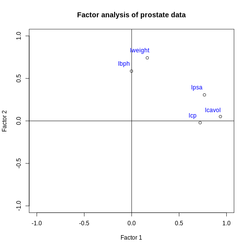
Similar to a biplot as we produced in the PCA episode, we can “plot the loadings”. This shows how each original variable contributes to each of the factors we chose to visualise.
R
#First, carry out factor analysis using two factors
pros_fa <- factanal(pros2, factors = 2)

#plot loadings for each factor
plot(
  pros_fa$loadings[, 1],
  pros_fa$loadings[, 2],
  xlab = "Factor 1",
  ylab = "Factor 2",
  ylim = c(-1, 1),
  xlim = c(-1, 1),
  main = "Factor analysis of prostate data"
)
abline(h = 0, v = 0)

#add column names to each point
text(
  pros_fa$loadings[, 1] - 0.08,
  pros_fa$loadings[, 2] + 0.08,
  colnames(pros2),
  col = "blue"
)
K-medoids (PAM)
One problem with K-means is that using the mean to define cluster centroids means that clusters can be very sensitive to outlying observations.
K-medoids, also known as “partitioning around medoids (PAM)” is similar to K-means, but uses the median rather than the mean as the method for defining cluster centroids. Using the median rather than the mean reduces sensitivity of clusters to outliers in the data.
K-medioids has had popular application in genomics, for example the well-known PAM50 gene set in breast cancer, which has seen some prognostic applications.
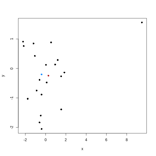
The following example shows how cluster centroids differ when created using medians rather than means.
R
x <- rnorm(20)
y <- rnorm(20)
x[10] <- x[10] + 10
plot(x, y, pch = 16)
points(mean(x), mean(y), pch = 16, col = "firebrick")
points(median(x), median(y), pch = 16, col = "dodgerblue")
PAM can be carried out using pam() from the
cluster package.
Challenge 2 (3 mins)
Use the output from your factor analysis and the plots above to interpret the results of your analysis.
What variables are most important in explaining each factor? Do you think this makes sense biologically? Consider or discuss in groups.
This plot suggests that the variables lweight and
lbph are associated with high values on factor 2 (but lower
values on factor 1) and the variables lcavol, lcp and lpsa are
associated with high values on factor 1 (but lower values on factor 2).
There appear to be two ‘clusters’ of variables which can be represented
by the two factors.
The grouping of weight and enlargement (lweight and lbph) makes sense biologically, as we would expect prostate enlargement to be associated with greater weight. The groupings of lcavol, lcp, and lpsa also make sense biologically, as larger cancer volume may be expected to be associated with greater cancer spread and therefore higher PSA in the blood.
Advantages and disadvantages of Factor Analysis
There are several advantages and disadvantages of using FA as a dimensionality reduction method.
Advantages:
- FA is a useful way of combining different groups of data into known representative factors, thus reducing dimensionality in a dataset.
- FA can take into account researchers’ expert knowledge when choosing the number of factors to use, and can be used to identify latent or hidden variables which may not be apparent from using other analysis methods.
- It is easy to implement with many software tools available to carry out FA.
- Confirmatory FA can be used to test hypotheses.
Disadvantages:
- Justifying the choice of number of factors to use may be difficult if little is known about the structure of the data before analysis is carried out.
- Sometimes, it can be difficult to interpret what factors mean after analysis has been completed.
- Like PCA, standard methods of carrying out FA assume that input variables are continuous, although extensions to FA allow ordinal and binary variables to be included (after transforming the input matrix).
Further reading
- Gundogdu et al. (2019) Comparison of performances of Principal Component Analysis (PCA) and Factor Analysis (FA) methods on the identification of cancerous and healthy colon tissues. International Journal of Mass Spectrometry 445:116204.
- Kustra et al. (2006) A factor analysis model for functional genomics. BMC Bioinformatics 7: doi:10.1186/1471-2105-7-21.
- Yong, A.G. & Pearce, S. (2013) A beginner’s guide to factor analysis: focusing on exploratory factor analysis. Tutorials in Quantitative Methods for Psychology 9(2):79-94.
- Confirmatory factor analysis can be carried out with the package Lavaan.
- A more sophisticated implementation of EFA is available in the packages EFA.dimensions and psych.
- Factor analysis is a method used for reducing dimensionality in a dataset by reducing variation contained in multiple variables into a smaller number of uncorrelated factors.
- PCA can be used to identify the number of factors to initially use in factor analysis.
- The
factanal()function in R can be used to fit a factor analysis, where the number of factors is specified by the user. - Factor analysis can take into account expert knowledge when deciding on the number of factors to use, but a disadvantage is that the output requires careful interpretation.