Explainability methods overview
Last updated on 2024-12-17 | Edit this page
Overview
Questions
- What are the major categories of explainability methods, and how do they differ?
- How do you determine which explainability method to use for a specific use case?
- What are the trade-offs between black-box and white-box approaches to explainability?
- How do post-hoc explanation methods compare to inherently interpretable models in terms of utility and reliability?
Objectives
- Understand the key differences between black-box and white-box explanation methods.
- Explore the trade-offs between post-hoc explainability and inherent interpretability in models.
- Identify and categorize different explainability techniques based on their scope, model access, and approach.
- Learn when to apply specific explainability techniques for various machine learning tasks.
Fantastic Explainability Methods and Where to Use Them
We will now take a bird’s-eye view of explainability methods that are widely applied on complex models like neural networks. We will get a sense of when to use which kind of method, and what the tradeoffs between these methods are.
Three axes of use cases for understanding model behavior
When deciding which explainability method to use, it is helpful to define your setting along three axes. This helps in understanding the context in which the model is being used, and the kind of insights you are looking to gain from the model.
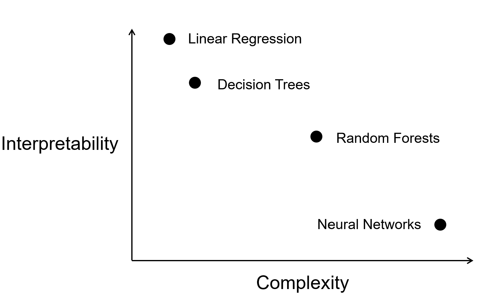
Inherently Interpretable vs Post Hoc Explainable
Understanding the tradeoff between interpretability and complexity is crucial in machine learning. Simple models like decision trees, random forests, and linear regression offer transparency and ease of understanding, making them ideal for explaining predictions to stakeholders. In contrast, neural networks, while powerful, lack interpretability due to their complexity. Post hoc explainable techniques can be applied to neural networks to provide explanations for predictions, but it’s essential to recognize that using such methods involves a tradeoff between model complexity and interpretability.
Striking the right balance between these factors is key to selecting the most suitable model for a given task, considering both its predictive performance and the need for interpretability.
Local vs Global Explanations
Local explanations focus on describing model behavior within a specific neighborhood, providing insights into individual predictions. Conversely, global explanations aim to elucidate overall model behavior, offering a broader perspective. While global explanations may be more comprehensive, they run the risk of being overly complex.
Both types of explanations are valuable for uncovering biases and ensuring that the model makes predictions for the right reasons. The tradeoff between local and global explanations has a long history in statistics, with methods like linear regression (global) and kernel smoothing (local) illustrating the importance of considering both perspectives in statistical analysis.
Local example: Understanding single prediciton using SHAP
SHAP (SHapley Additive exPlanations) is a feature attribution method that provides insights into how individual features contribute to a specific prediction for an individual instance. Its popularity stems from its strong theoretical foundation and flexibility, making it applicable across a wide range of machine learning models, including tree-based models, linear regressions, and neural networks. SHAP is particularly relevant for deep learning models, where traditional feature importance methods struggle to handle complex feature interactions and non-linearities.
Examples
- Explaining why a specific patient was predicted to have a high risk of developing a disease.
- Identifying the key features driving the predicted price of a single house in a real estate model.
- Understanding why a fraud detection model flagged a particular transaction as suspicious
How it works: SHAP values start with a model that’s been fitted to all features and training data. We then perturb the instance by including or excluding features, where excluding a feature means replacing its value with a baseline value (i.e., its average value or a value sampled from the dataset). For each subset of features, SHAP computes the model’s prediction and measures the marginal contribution of each feature to the outcome. To ensure fairness and consistency, SHAP averages these contributions across all possible feature orderings. The result is a set of SHAP values that explain how much each feature pushed the prediction higher or lower relative to the baseline model output. These local explanations provide clear, human-readable insights into why the model made a particular prediction. However, for high-dimensional datasets, the combinatorial nature of feature perturbations can lead to longer compute times, making approximations like Kernel SHAP more practical.
Global example: Aggregated insights with SHAP
SHAP (SHapley Additive exPlanations) can also provide global insights by aggregating feature attributions across multiple instances, offering a comprehensive understanding of a model’s behavior. Its ability to rank feature importance and reveal trends makes it invaluable for uncovering dataset-wide patterns and detecting potential biases. This global perspective is particularly useful for complex models where direct interpretation of weights or architecture is not feasible.
Examples
- Understanding which features are the most influential across a dataset (e.g., income level being the most significant factor in loan approvals).
- Detecting global trends or biases in a predictive model, such as gender-based discrepancies in hiring recommendations.
- Identifying the key drivers behind a model’s success in predicting customer churn rates.
How it works: SHAP values are first computed for individual predictions by analyzing the contributions of features to specific outputs. These local attributions are then aggregated across all instances in the dataset to compute a global measure of feature importance. For example, averaging the absolute SHAP values for each feature reveals its overall impact on the model’s predictions. This process allows practitioners to identify which features consistently drive predictions and uncover dataset-level insights. By connecting local explanations to a broader view, SHAP provides a unified approach to understanding both individual predictions and global model behavior.
However, for large datasets or highly complex models, aggregating SHAP values can be computationally expensive. Optimized implementations, such as Tree SHAP for tree-based models, help mitigate this challenge by efficiently calculating global feature attributions.
Black box vs White Box Approaches
Techniques that require access to model internals (e.g., model architecture and model weights) are called “white box” while techniques that only need query access to the model are called “black box”. Even without access to the model weights, black box or top down approaches can shed a lot of light on model behavior. For example, by simply evaluating the model on certain kinds of data, high level biases or trends in the model’s decision making process can be unearthed.
White box approaches use the weights and activations of the model to understand its behavior. These classes or methods are more complex and diverse, and we will discuss them in more detail later in this episode. Some large models are closed-source due to commercial or safety concerns; for example, users can’t get access to the weights of GPT-4. This limits the use of white box explanations for such models.
Classes of Explainability Methods for Understanding Model Behavior
Diagnostic Testing
This is the simplest approach towards explaining model behavior. This involves applying a series of unit tests to the model, where each test is a sample input where you know what the correct output should be. By identifying test examples that break the heuristics the model relies on (called counterfactuals), you can gain insights into the high-level behavior of the model.
Example Methods: Counterfactuals, Unit tests
Pros and Cons: These methods allow for gaining insights into the high-level behavior of the model without the needing access to model weights. This is especially useful with recent powerful closed-source models like GPT-4. One challenge with this approach is that it is hard to identify in advance what heuristics a model may depend on.
Baking interpretability into models
Some recent research has focused on tweaking highly complex models like neural networks, towards making them more interpretable inherently. One such example with language models involves training the model to generate rationales for its prediction, in addition to its original prediction. This approach has gained some traction, and there are even public benchmarks for evaluating the quality of these generated rationales.
Example methods: Rationales with WT5, Older approaches for rationales
Pros and cons: These models hope to achieve the best of both worlds: complex models that are also inherently interpretable. However, research in this direction is still new, and there are no established and reliable approaches for real world applications just yet.
Identifying Decision Rules of the Model:
In this class of methods, we try find a set of rules that generally explain the decision making process of the model. Loosely, these rules would be of the form “if a specific condition is met, then the model will predict a certain class”.
Example methods: Anchors, Universal Adversarial Triggers
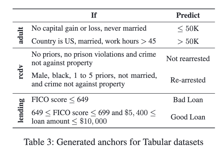
Pros and cons: Some global rules help find “bugs” in the model, or identify high level biases. But finding such broad coverage rules is challenging. Furthermore, these rules only showcase the model’s weaknesses, but give next to no insight as to why these weaknesses exist.
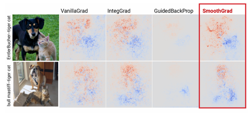
Visualizing model weights or representations
Just like how a picture tells a thousand words, visualizations can help encapsulate complex model behavior in a simple image. Visualizations are commonly used in explaining neural networks, where the weights or data representations of the model are directly visualized. Many such approaches involve reducing the high-dimensional weights or representations to a 2D or 3D space, using techniques like PCA, tSNE, or UMAP. Alternatively, these visualizations can retain their high dimensional representation, but use color or size to identify which dimensions or neurons are more important.
Example methods: Visualizing attention heatmaps, Weight visualizations, Model activation visualizations
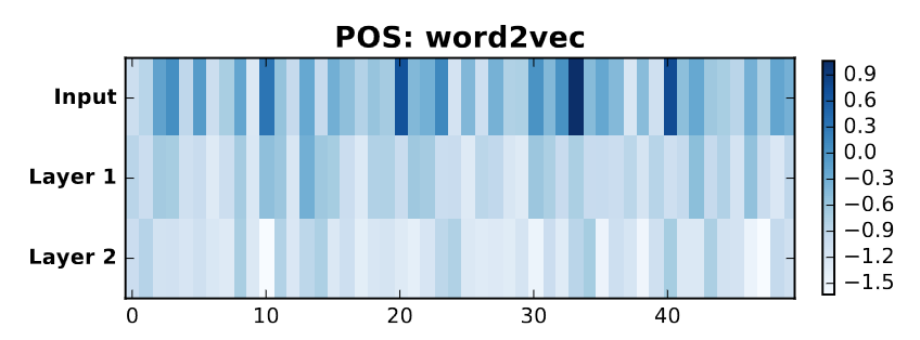
Pros and cons: Gleaning model behaviour from visualizations is very intuitive and user-friendly, and visualizations sometimes have interactive interfaces. However, visualizations can be misleading, especially when high-dimensional vectors are reduced to 2D, leading to a loss of information (crowding issue).
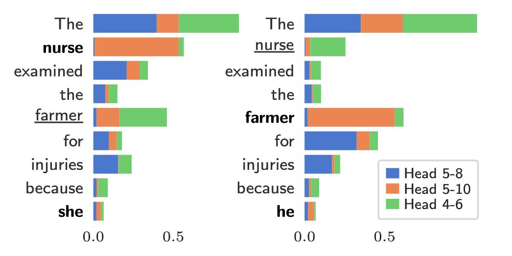
An iconic debate exemplifying the validity of visualizations has centered around attention heatmaps. Research has shown them to be unreliable, and then reliable again. (Check out the titles of these papers!) Thus, visualization can only be used as an additional step in an analysis, and not as a standalone method.
Understanding the impact of training examples
These techniques unearth which training data instances caused the model to generate a specific prediction for a given sample. At a high level, these techniques mathematically identify what training samples that – if removed from the training process – are most influential for causing a particular prediction.
Example methods: Influence functions, Representer point selection
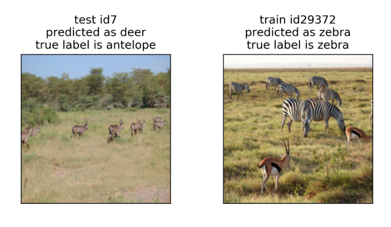
Pros and cons: The insights from these approaches are actionable - by identifying the data responsible for a prediction, it can help correct labels or annotation artifacts in that data. Unfortunately, these methods scale poorly with the size of the model and training data, quickly becoming computationally expensive. Furthermore, even knowing which datapoints had a high influence on a prediction, we don’t know what it was about that datapoint that caused the influence.
Understanding the impact of a single example:
For a single input, what parts of the input were most important in generating the model’s prediction? These methods study the signal sent by various features to the model, and observe how the model reacts to changes in these features.
Example methods: Saliency Maps, LIME/SHAP, Perturbations (Input reduction, Adversarial Perturbations)
These methods can be further subdivided into two categories: gradient-based methods that rely on white-box model access to directly see the impact of changing a single input, and perturbation-based methods that manually perturb an input and re-query the model to see how the prediction changes.
Pros and cons: These methods are fast to compute, and flexible in their use across models. However, the insights gained from these methods are not actionable - knowing which part of the input caused the prediction does not highlight why that part caused it. On finding issues in the prediction process, it is also hard to pick up on if there is an underlying issue in the model, or just the specific inputs tested on. Relatedly, these methods can be unstable, and can even be fooled by adversarial examples.
Probing internal representations
As the name suggests, this class of methods aims to probe the internals of a model, to discover what kind of information or knowledge is stored inside the model. Probes are often administered to a specific component of the model, like a set of neurons or layers within a neural network.
Example methods: Probing classifiers, Causal tracing
Pros and cons: Probes have shown that it is possible to find highly interpretable components in a complex model, e.g., MLP layers in transformers have been shown to store factual knowledge in a structured manner. However, there is no systematic way of finding interpretable components, and many components may remain elusive to humans to understand. Furthermore, the model components that have been shown to contain certain knowledge may not actually play a role in the model’s prediction.
Is that all?
Nope! We’ve discussed a few of the common explanation techniques, but many others exist. In particular, specialized model architectures often need their own explanation algorithms. For instance, Yuan et al. give an overview of different explanation techniques for graph neural networks (GNNs).
Classifying explanation techniques
For each of the explanation techniques described above, discuss the following with a partner:
- Does it require black-box or white-box model access?
- Are the explanations it provides global or local?
- Is the technique post-hoc or does it rely on inherent interpretability of the model?
| Approach | Post Hoc or Inherently Interpretable? | Local or Global? | White Box or Black Box? |
|---|---|---|---|
| Diagnostic Testing | Post Hoc | Global | Black Box |
| Baking interpretability into models | Inherently Interpretable | Local | White Box |
| Identifying Decision Rules of the Model | Post Hoc | Both | White Box |
| Visualizing model weights or representations | Post Hoc | Global | White Box |
| Understanding the impact of training examples | Post Hoc | Local | White Box |
| Understanding the impact of a single example | Post Hoc | Local | Both |
| Probing internal representations of a model | Post Hoc | Global/Local | White Box |
What explanation should you use when? There is no simple answer, as it depends upon your goals (i.e., why you need an explanation), who the audience is, the model architecture, and the availability of model internals (e.g., there is no white-box access to ChatGPT unless you work for Open AI!). The next exercise asks you to consider different scenarios and discuss what explanation techniques are appropriate.
Challenge
Think about the following scenarios and suggest which explainability method would be most appropriate to use, and what information could be gained from that method. Furthermore, think about the limitations of your findings.
Note: These are open-ended questions, and there is no correct answer. Feel free to break into discussion groups to discuss the scenarios.
Scenario 1: Suppose that you are an ML engineer working at a tech company. A fast-food chain company consults with you about sentimental analysis based on feedback they collected on Yelp and their survey. You use an open sourced LLM such as Llama-2 and finetune it on the review text data. The fast-food company asks to provide explanations for the model: Is there any outlier review? How does each review in the data affect the finetuned model? Which part of the language in the review indicates that a customer likes or dislikes the food? Can you score the food quality according to the reviews? Does the review show a trend over time? What item is gaining popularity or losing popularity? Q: Can you suggest a few explainability methods that may be useful for answering these questions?
Scenario 2: Suppose that you are a radiologist who analyzes medical images of patients with the help of machine learning models. You use black-box models (e.g., CNNs, Vision Transformers) to complement human expertise and get useful information before making high-stake decisions. Which areas of a medical image most likely explains the output of a black-box? Can we visualize and understand what features are captured by the intermediate components of the black-box models? How do we know if there is a distribution shift? How can we tell if an image is an out-of-distribution example? Q: Can you suggest a few explainability methods that may be useful for answering these questions?
Scenario 3: Suppose that you work on genomics and you just collected samples of single-cell data into a table: each row records gene expression levels, and each column represents a single cell. You are interested in scientific hypotheses about evolution of cells. You believe that only a few genes are playing a role in your study. What exploratory data analysis techniques would you use to examine the dataset? How do you check whether there are potential outliers, irregularities in the dataset? You believe that only a few genes are playing a role in your study. What can you do to find the set of most explanatory genes? How do you know if there is clustering, and if there is a trajectory of changes in the cells? Q: Can you explain the decisions you make for each method you use?
Summary
There are many available explanation techniques and they differ along three dimensions: model access (white-box or black-box), explanation scope (global or local), and approach (inherently interpretable or post-hoc). There’s often no objectively-right answer of which explanation technique to use in a given situation, as the different methods have different tradeoffs.
References and Further Reading
This lesson provides a gentle overview into the world of explainability methods. If you’d like to know more, here are some resources to get you started:
- Tutorials on Explainability:
- Wallace, E., Gardner, M., & Singh, S. (2020, November). Interpreting predictions of NLP models. In Proceedings of the 2020 Conference on Empirical Methods in Natural Language Processing: Tutorial Abstracts (pp. 20-23).
- Lakkaraju, H., Adebayo, J., & Singh, S. (2020). Explaining machine learning predictions: State-of-the-art, challenges, and opportunities. NeurIPS Tutorial.
- Belinkov, Y., Gehrmann, S., & Pavlick, E. (2020, July). Interpretability and analysis in neural NLP. In Proceedings of the 58th annual meeting of the association for computational linguistics: tutorial abstracts (pp. 1-5).
- Research papers: