Gene set enrichment analysis
Last updated on 2026-07-14 | Edit this page
Overview
Questions
- What is the aim of performing gene set enrichment analysis?
- What is the method of over-representation analysis?
- What are the commonly-used gene set databases?
Objectives
- Learn the method of gene set enrichment analysis.
- Learn how to obtain gene sets from various resources in R.
- Learn how to perform gene set enrichment analysis and how to visualize enrichment results.
After we have obtained a list of differentially expressed (DE) genes, the next question naturally to ask is what biological functions these DE genes may affect. Gene set enrichment analysis (GSEA) evaluates the associations of a list of DE genes to a collection of pre-defined gene sets, where each gene set has a specific biological meaning. Once DE genes are significantly enriched in a gene set, the conclusion is made that the corresponding biological meaning (e.g. a biological process or a pathway) is significantly affected.
The definition of a gene set is very flexible and the construction of gene sets is straightforward. In most cases, gene sets are from public databases where huge efforts from scientific curators have already been made to carefully categorize genes into gene sets with clear biological meanings. Nevertheless, gene sets can also be self-defined from individual studies, such as a set of genes in a network module from a co-expression network analysis, or a set of genes that are up-regulated in a certain disease.
There are a huge amount of methods available for GSEA analysis. In this episode, we will learn the simplest but the mostly used one: the over-representation analysis (ORA). ORA is directly applied to the list of DE genes and it evaluates the association of the DE genes and the gene set by the numbers of genes in different categories.
Please note, ORA is a universal method that it can not only be applied to the DE gene list, but also any type of gene list of interest to look for their statistically associated biological meanings.
In this episode, we will start with a tiny example to illustrate the statistical method of ORA. Next we will go through several commonly-used gene set databases and how to access them in R. Then, we will learn how to perform ORA analysis with the Bioconductor package clusterProfiler. And in the end, we will learn several visualization methods on the GSEA results.
Following is a list of packages that will be used in this episode:
R
library(SummarizedExperiment)
library(DESeq2)
library(gplots)
library(microbenchmark)
library(org.Hs.eg.db)
library(org.Mm.eg.db)
library(msigdb)
library(clusterProfiler)
library(enrichplot)
library(ggplot2)
library(simplifyEnrichment)
The statistical method
To demonstrate the ORA analysis, we use a list of DE genes from a
comparison between genders. The following code performs
DESeq2 analysis which you should have already learnt in
the previous episode. In the end, we have a list of DE genes filtered by
FDR < 0.05, and save it in the object sexDEgenes.
The file data/GSE96870_se.rds contains a
RangedSummarizedExperiment that contains RNA-Seq counts
that were downloaded in Episode 2 and
constructed in Episode 3 (minimal
codes for downloading and constructing in the script download_data.R.
In the following code, there are also comments that explain every step
of the analysis.
R
library(SummarizedExperiment)
library(DESeq2)

# read the example dataset which is a `RangedSummarizedExperiment` object
se <- readRDS("data/GSE96870_se.rds")

# only restrict to mRNA (protein-coding genes)
se <- se[rowData(se)$gbkey == "mRNA"]

# construct a `DESeqDataSet` object where we also specify the experimental design
dds <- DESeqDataSet(se, design = ~ sex + time)
# perform DESeq2 analysis
dds <- DESeq(dds)
# obtain DESeq2 results, here we only want Male vs Female in the "sex" variable
resSex <- results(dds, contrast = c("sex", "Male", "Female"))
# extract DE genes with padj < 0.05
sexDE <- as.data.frame(subset(resSex, padj < 0.05))
# the list of DE genes
sexDEgenes <- rownames(sexDE)
Let’s check the number of DE genes and how they look like. It seems the number of DE genes is very small, but it is OK for this example.
R
length(sexDEgenes)
OUTPUT
[1] 54R
head(sexDEgenes)
OUTPUT
[1] "Lgr6" "Myoc" "Fibcd1" "Kcna4" "Ctxn2" "S100a9"Next we construct a gene set which contains genes on sex chromosomes
(let’s call it the “XY gene set”). Recall the
RangedSummarizedExperiment object also includes genomic
locations of genes, thus we can simply obtain sex genes by filtering the
chromosome names.
In the following code, geneGR is a GRanges
object on which seqnames() is applied to extract chromosome
names. seqnames() returns a special data format and we need
to explicitly convert it to a normal vector by
as.vector().
R
geneGR <- rowRanges(se)
totalGenes <- rownames(se)
XYGeneSet <- totalGenes[as.vector(seqnames(geneGR)) %in% c("X", "Y")]
head(XYGeneSet)
OUTPUT
[1] "Gm21950" "Gm14346" "Gm14345" "Gm14351" "Spin2-ps1" "Gm3701" R
length(XYGeneSet)
OUTPUT
[1] 1134The format of a single gene set is very straightforward, which is simply a vector. The ORA analysis is applied on the DE gene vector and gene set vector.
Before we move on, one thing worth to mention is that ORA deals with
two gene vectors. To correctly map between them, gene ID types must be
consistent in the two vectors. In this tiny example, since both DE genes
and the XY gene set are from the same object se,
they are ensured to be in the same gene ID types (the gene symbol). But
in general, DE genes and gene sets are from two different sources
(e.g. DE genes are from researcher’s experiment and gene sets are from
public databases), it is very possible that gene IDs are not consistent
in the two. Later in this episode, we will learn how to perform gene ID
conversion in the ORA analysis.
Since the DE genes and the gene set can be mathematically thought of as two sets, a natural way is to first visualize them with a Venn diagram.
R
library(gplots)
plot(venn(list("sexDEgenes"  = sexDEgenes,
               "XY gene set" = XYGeneSet)))
title(paste0("|universe| = ", length(totalGenes)))
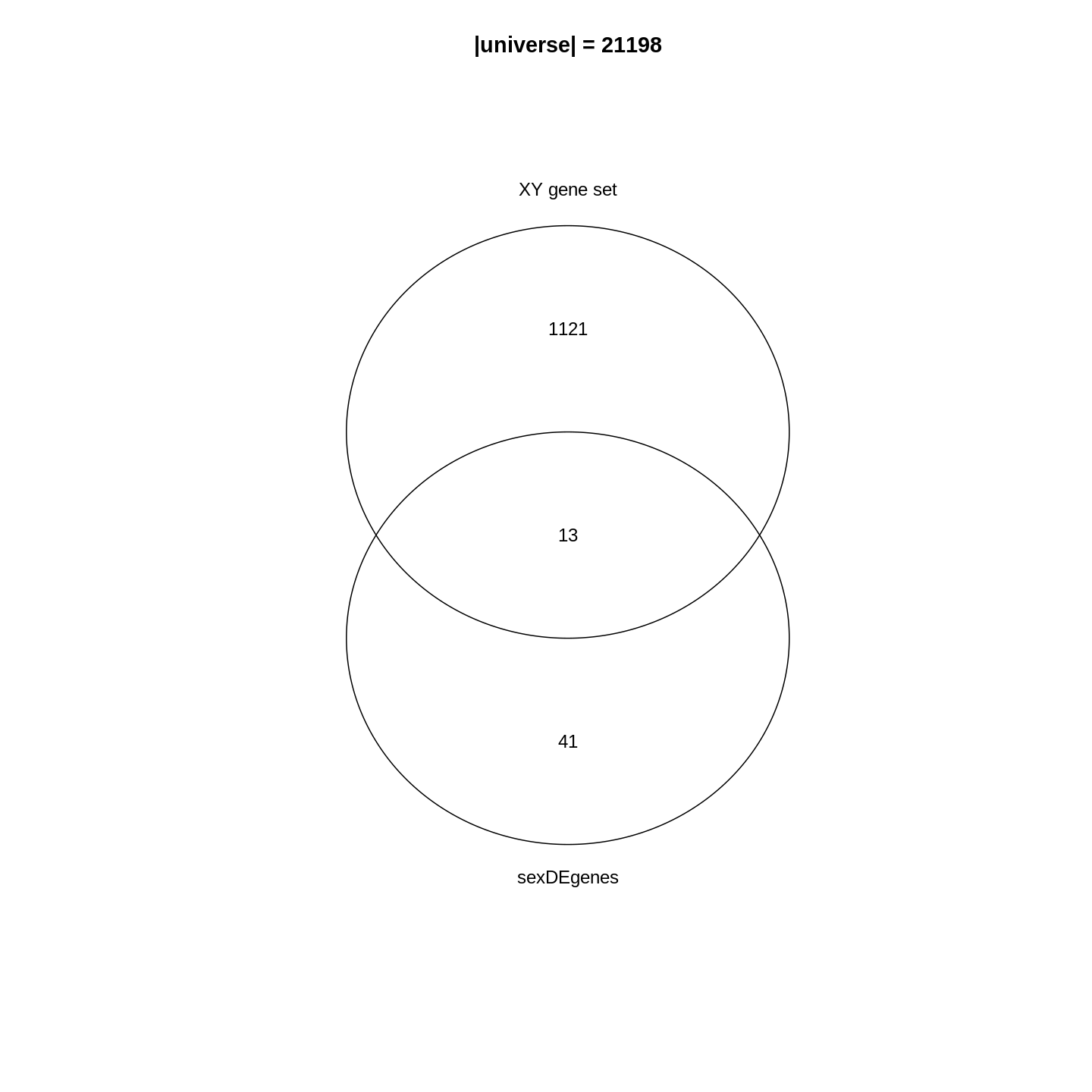
In the Venn diagram, we can observe that around 1.1% (13/1134) of genes in the XY gene set are DE. Compared to the global fraction of DE genes (54/21198 = 0.25%), it seems there is a strong relations between DE genes and the gene set. We can also compare the fraction of DE genes that belong to the gene set (13/54 = 24.1%) and the global fraction of XY gene set in the genome (1134/21198 = 5.3%). On the other hand, it is quite expected because the two events are actually biologically relevant where one is from a comparison between genders and the other is the set of gender-related genes.
Then, how to statistically measure the enrichment or over-representation? Let’s go to the next section.
Fisher’s exact test
To statistically measure the enrichment, the relationship of DE genes and the gene set is normally formatted into the following 2x2 contingency table, where in the table are the numbers of genes in different categories. \(n_{+1}\) is the size of the XY gene set (i.e. the number of member genes), \(n_{1+}\) is the number of DE genes, \(n\) is the number of total genes.
| In the gene set | Not in the gene set | Total | |
|---|---|---|---|
| DE | \(n_{11}\) | \(n_{12}\) | \(n_{1+}\) |
| Not DE | \(n_{21}\) | \(n_{22}\) | \(n_{2+}\) |
| Total | \(n_{+1}\) | \(n_{+2}\) | \(n\) |
These numbers can be obtained as in the following code1. Note we replace
+ with 0 in the R variable names.
R
n    <- nrow(se)
n_01 <- length(XYGeneSet)
n_10 <- length(sexDEgenes)
n_11 <- length(intersect(sexDEgenes, XYGeneSet))
Other values can be obtained by:
R
n_12 <- n_10 - n_11
n_21 <- n_01 - n_11
n_20 <- n    - n_10
n_02 <- n    - n_01
n_22 <- n_02 - n_12
All the values are:
R
matrix(c(n_11, n_12, n_10, n_21, n_22, n_20, n_01, n_02, n),
    nrow = 3, byrow = TRUE)
OUTPUT
     [,1]  [,2]  [,3]
[1,]   13    41    54
[2,] 1121 20023 21144
[3,] 1134 20064 21198
And we fill these numbers into the 2x2 contingency table:
| In the gene set | Not in the gene set | Total | |
|---|---|---|---|
| DE | 13 | 41 | 54 |
| Not DE | 1121 | 20023 | 21144 |
| Total | 1134 | 20064 | 21198 |
Fisher’s exact test can be used to test the associations of the two
marginal attributes, i.e. is there a dependency of a gene to be a DE
gene and to be in the XY gene set? In R, we can use the
function fisher.test() to perform the test. The input is
the top-left 2x2 sub-matrix. We specify
alternative = "greater" in the function because we are only
interested in over-representation.
R
fisher.test(matrix(c(n_11, n_12, n_21, n_22), nrow = 2, byrow = TRUE),
    alternative = "greater")
OUTPUT
	Fisher's Exact Test for Count Data

data:  matrix(c(n_11, n_12, n_21, n_22), nrow = 2, byrow = TRUE)
p-value = 3.906e-06
alternative hypothesis: true odds ratio is greater than 1
95 percent confidence interval:
 3.110607      Inf
sample estimates:
odds ratio
  5.662486
In the output, we can see the p-value is very small
(3.906e-06), then we can conclude DE genes have a very
strong enrichment in the XY gene set.
Results of the Fisher’s Exact test can be saved into an object
t, which is a simple list, and the p-value can be
obtained by t$p.value.
R
t <- fisher.test(matrix(c(n_11, n_12, n_21, n_22), nrow = 2, byrow = TRUE),
    alternative = "greater")
t$p.value
OUTPUT
[1] 3.9059e-06Odds ratio from the Fisher’s exact test is defined as follows:
\[ \mathrm{Odds\_ratio} = \frac{n_{11}/n_{21}}{n_{12}/n_{22}} = \frac{n_{11}/n_{12}}{n_{21}/n_{22}} = \frac{n_{11} * n_{22}}{n_{12} * n_{21}} \]
If there is no association between DE genes and the gene set, odds ratio is expected to be 1. And it is larger than 1 if there is an over-representation of DE genes on the gene set.
Further reading
The 2x2 contingency table can be transposed and it does not affect the Fisher’s exact test. E.g. let’s put whether genes are in the gene sets on rows, and put whether genes are DE on columns.
| DE | Not DE | Total | |
|---|---|---|---|
| In the gene set | 13 | 1121 | 1134 |
| Not in the gene set | 41 | 20023 | 20064 |
| Total | 54 | 21144 | 21198 |
And the corresponding fisher.test() is:
R
fisher.test(matrix(c(13, 1121, 41, 20023), nrow = 2, byrow = TRUE),
    alternative = "greater")
OUTPUT
	Fisher's Exact Test for Count Data

data:  matrix(c(13, 1121, 41, 20023), nrow = 2, byrow = TRUE)
p-value = 3.906e-06
alternative hypothesis: true odds ratio is greater than 1
95 percent confidence interval:
 3.110607      Inf
sample estimates:
odds ratio
  5.662486
The hypergeometric distribution
We can look at the problem from another aspect. This time we treat all genes as balls in a big box where all the genes have the same probability to be picked up. Some genes are marked as DE genes (in red in the figure) and other genes are marked as non-DE genes (in blue). We grab \(n_{+1}\) genes (the size of the gene set) from the box and we want to ask what is the probability of having \(n_{11}\) DE genes in our hand?
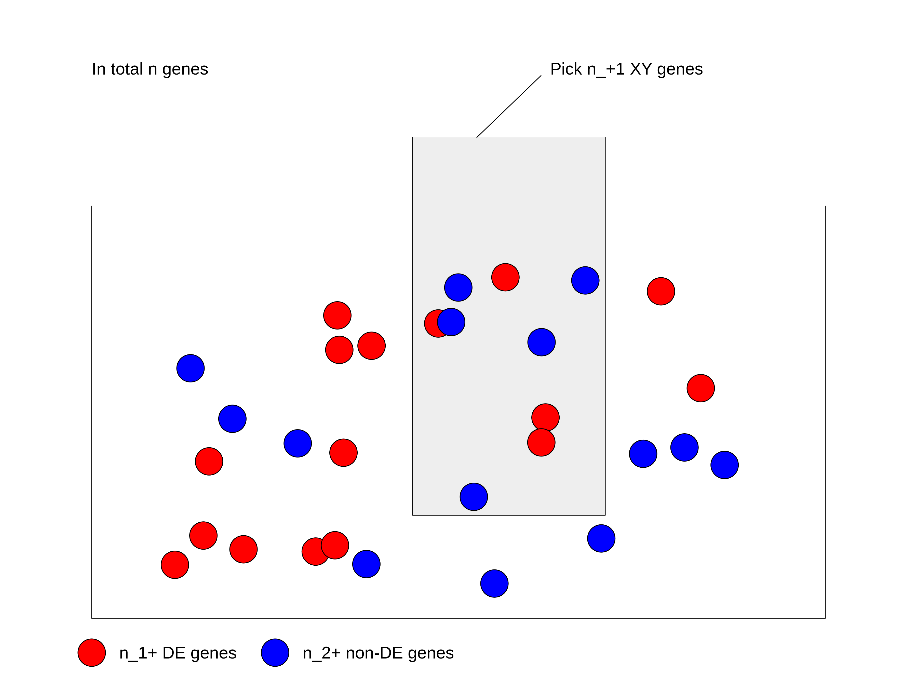
We first calculate the total number of ways of picking \(n_{+1}\) genes from total \(n\) genes, without distinguishing whether they are DE or not: \(\binom{n}{n_{+1}}\).
Next, in the \(n_{+1}\) genes that have been picked, there are \(n_{11}\) DE genes which can only be from the total \(n_{1+}\) DE genes. Then the number of ways of picking \(n_{11}\) DE genes from \(n_{1+}\) total DE genes is \(\binom{n_{1+}}{n_{11}}\).
Similarly, there are still \(n_{21}\) non-DE genes in our hand, which can only be from the total \(n_{2+}\) non-DE genes. Then the number of ways of picking \(n_{21}\) non-DE genes from \(n_{2+}\) total non-DE genes: \(\binom{n_{2+}}{n_{21}}\).
Since picking DE genes and picking non-DE genes are independent, the number of ways of picking \(n_{+1}\) genes which contain \(n_{11}\) DE genes and \(n_{21}\) non-DE genes is their multiplication: \(\binom{n_{1+}}{n_{11}} \binom{n_{2+}}{n_{21}}\).
And the probability \(P\) is:
\[P = \frac{\binom{n_{1+}}{n_{11}} \binom{n_{2+}}{n_{21}}}{\binom{n}{n_{+1}}} = \frac{\binom{n_{1+}}{n_{11}} \binom{n - n_{1+}}{n_{+1} -n_{11}}}{\binom{n}{n_{+1}}} \]
where in the denominator is the number of ways of picking \(n_{+1}\) genes without distinguishing whether they are DE or not.
If \(n\) (number of total genes), \(n_{1+}\) (number of DE genes) and \(n_{+1}\) (size of gene set) are all fixed values, the number of DE genes that are picked can be denoted as a random variable \(X\). Then \(X\) follows the hypergeometric distribution with parameters \(n\), \(n_{1+}\) and \(n_{+1}\), written as:
\[ X \sim \mathrm{Hyper}(n, n_{1+}, n_{+1})\]
The p-value of the enrichment is calculated as the probability of having an observation equal to or larger than \(n_{11}\) under the assumption of independence:
\[ \mathrm{Pr}( X \geqslant n_{11} ) = \sum_{x \in \{ {n_{11}, n_{11}+1, ..., \min\{n_{1+}, n_{+1}\} \}}} \mathrm{Pr}(X = x) \]
In R, the function phyper() calculates p-values
from the hypergeometric distribution. There are four arguments:
R
phyper(q, m, n, k)
which are:
-
q: the observation, -
m: number of DE genes, -
n: number of non-DE genes, -
k: size of the gene set.
phyper() calculates \(\mathrm{Pr}(X \leqslant q)\). To calculate
\(\mathrm{Pr}(X \geqslant q)\), we need
to transform it a little bit:
\[ \mathrm{Pr}(X \geqslant q) = 1 - \mathrm{Pr}(X < q) = 1 - \mathrm{Pr}(X \leqslant q-1)\]
Then, the correct use of phyper() is:
R
1 - phyper(q - 1, m, n, k)
Let’s plugin our variables:
R
1 - phyper(n_11 - 1, n_10, n_20, n_01)
OUTPUT
[1] 3.9059e-06Optionally, lower.tail argument can be specified which
directly calculates p-values from the upper tail of the
distribution.
R
phyper(n_11 - 1, n_10, n_20, n_01, lower.tail = FALSE)
OUTPUT
[1] 3.9059e-06If we switch n_01 and n_10, the
p-values are identical:
R
1 - phyper(n_11 - 1, n_01, n_02, n_10)
OUTPUT
[1] 3.9059e-06fisher.test() and phyper() give the same
p-value. Actually the two methods are identical because in
Fisher’s exact test, hypergeometric distribution is the exact
distribution of its statistic.
Let’s test the runtime of the two functions:
R
library(microbenchmark)
microbenchmark(
    fisher = fisher.test(matrix(c(n_11, n_12, n_21, n_22), nrow = 2, byrow = TRUE),
        alternative = "greater"),
    hyper = 1 - phyper(n_11 - 1, n_10, n_20, n_01)
)
OUTPUT
Unit: microseconds
   expr     min       lq      mean   median       uq     max neval
 fisher 261.349 265.3810 277.03629 270.6155 286.1945 493.071   100
  hyper   1.693   1.8985   3.05905   3.2060   3.5315  21.220   100
It is very astonishing that phyper() is hundreds of
times faster than fisher.test(). Main reason is in
fisher.test(), there are many additional calculations
besides calculating the p-value. So if you want to implement
ORA analysis by yourself, always consider to use phyper()2.
Further reading
Current tools also use Binomial distribution or chi-square test for ORA analysis. These two are just approximations. Please refer to Rivals et al., Enrichment or depletion of a GO category within a class of genes: which test? Bioinformatics 2007 which gives an overview of statistical methods used in ORA analysis.
Gene set resources
We have learnt the basic methods of ORA analysis. Now we go to the second component of the analysis: the gene sets.
Gene sets represent prior knowledge of what is the general shared biological attribute of genes in the gene set. For example, in a “cell cycle” gene set, all the genes are involved in the cell cycle process. Thus, if DE genes are significantly enriched in the “cell cycle” gene set, which means there are significantly more cell cycle genes differentially expressed than expected, we can conclude that the normal function of cell cycle process may be affected.
As we have mentioned, genes in the gene set share the same “biological attribute” where “the attribute” will be used for making conclusions. The definition of “biological attribute” is very flexible. It can be a biological process such as “cell cycle”. It can also be from a wide range of other definitions, to name a few:
- Locations in the cell, e.g. cell membrane or cell nucleus.
- Positions on chromosomes, e.g. sex chromosomes or the cytogenetic band p13 on chromome 10.
- Target genes of a transcription factor or a microRNA, e.g. all genes that are transcriptionally regulationed by NF-κB.
- Signature genes in a certain tumor type, i.e. genes that are uniquely highly expressed in a tumor type.
The MSigDB database contains gene sets in many topics. We will introduce it later in this section.
You may have encountered many different ways to name gene sets: “gene sets”, “biological terms”, “GO terms”, “GO gene sets”, “pathways”, and so on. They basically refer to the same thing, but from different aspects. As shown in the following figure, “gene set” corresponds to a vector of genes and it is the representation of the data for computation. “Biological term” is a textual entity that contains description of its biological meaning; It corresponds to the knowledge of the gene set and is for the inference of the analysis. “GO gene sets” and “pathways” specifically refer to the enrichment analysis using GO gene sets and pahtway gene sets.

Before we touch the gene set databases, we first summarize the general formats of gene sets in R. In most analysis, a gene set is simply treated as a vector of genes. Thus, naturally, a collection of gene sets can be represented as a list of vectors. In the following example, there are three gene sets with 3, 5 and 2 genes. Some genes exist in multiple gene sets.
R
lt <- list(gene_set_1 = c("gene_1", "gene_2", "gene_3"),
           gene_set_2 = c("gene_1", "gene_3", "gene_4", "gene_5", "gene_6"),
           gene_set_3 = c("gene_4", "gene_7")
)
lt
OUTPUT
$gene_set_1
[1] "gene_1" "gene_2" "gene_3"

$gene_set_2
[1] "gene_1" "gene_3" "gene_4" "gene_5" "gene_6"

$gene_set_3
[1] "gene_4" "gene_7"
It is also very common to store the relations of gene sets and genes as a two-column data frame. The order of the gene set column and the gene column, i.e. which column locates as the first column, are quite arbitrary. Different tools may require differently.
R
data.frame(gene_set = rep(names(lt), times = sapply(lt, length)),
           gene = unname(unlist(lt)))
OUTPUT
     gene_set   gene
1  gene_set_1 gene_1
2  gene_set_1 gene_2
3  gene_set_1 gene_3
4  gene_set_2 gene_1
5  gene_set_2 gene_3
6  gene_set_2 gene_4
7  gene_set_2 gene_5
8  gene_set_2 gene_6
9  gene_set_3 gene_4
10 gene_set_3 gene_7
Or genes be in the first column:
OUTPUT
     gene   gene_set
1  gene_1 gene_set_1
2  gene_2 gene_set_1
3  gene_3 gene_set_1
4  gene_1 gene_set_2
5  gene_3 gene_set_2
6  gene_4 gene_set_2
7  gene_5 gene_set_2
8  gene_6 gene_set_2
9  gene_4 gene_set_3
10 gene_7 gene_set_3
Not very often, gene sets are represented as a matrix where one dimension corresponds to gene sets and the other dimension corresponds to genes. The values in the matix are binary where a value of 1 represents the gene is a member of the corresponding gene sets. In some methods, 1 is replaced by \(w_{ij}\) to weight the effect of the genes in the gene set.
#            gene_1 gene_2 gene_3 gene_4
# gene_set_1      1      1      0      0
# gene_set_2      1      0      1      1
Challenge
Can you convert between different gene set representations? E.g. convert a list to a two-column data frame?
R
lt <- list(gene_set_1 = c("gene_1", "gene_2", "gene_3"),
           gene_set_2 = c("gene_1", "gene_3", "gene_4", "gene_5", "gene_6"),
           gene_set_3 = c("gene_4", "gene_7")
)
To convert lt to a data frame (e.g. let’s put gene sets
in the first column):
R
df = data.frame(gene_set = rep(names(lt), times = sapply(lt, length)),
                gene = unname(unlist(lt)))
df
OUTPUT
     gene_set   gene
1  gene_set_1 gene_1
2  gene_set_1 gene_2
3  gene_set_1 gene_3
4  gene_set_2 gene_1
5  gene_set_2 gene_3
6  gene_set_2 gene_4
7  gene_set_2 gene_5
8  gene_set_2 gene_6
9  gene_set_3 gene_4
10 gene_set_3 gene_7
To convert df back to the list:
R
split(df$gene, df$gene_set)
OUTPUT
$gene_set_1
[1] "gene_1" "gene_2" "gene_3"

$gene_set_2
[1] "gene_1" "gene_3" "gene_4" "gene_5" "gene_6"

$gene_set_3
[1] "gene_4" "gene_7"
Next, let’s go through gene sets from several major databases: the GO, KEGG and MSigDB databases.
Gene Ontology gene sets
Gene Ontology (GO) is the standard source for gene set enrichment analysis. GO contains three namespaces of biological process (BP), cellular components (CC) and molecular function (MF) which describe a biological entity from different aspect. The associations between GO terms and genes are integrated in the Bioconductor standard packages: the organism annotation packages. In the current Bioconductor release, there are the following organism packages:
| Package | Organism | Package | Organism |
|---|---|---|---|
| org.Hs.eg.db | Human | org.Mm.eg.db | Mouse |
| org.Rn.eg.db | Rat | org.Dm.eg.db | Fly |
| org.At.tair.db | Arabidopsis | org.Dr.eg.db | Zebrafish |
| org.Sc.sgd.db | Yeast | org.Ce.eg.db | Worm |
| org.Bt.eg.db | Bovine | org.Gg.eg.db | Chicken |
| org.Ss.eg.db | Pig | org.Mmu.eg.db | Rhesus |
| org.Cf.eg.db | Canine | org.EcK12.eg.db | E coli strain K12 |
| org.Xl.eg.db | Xenopus | org.Pt.eg.db | Chimp |
| org.Ag.eg.db | Anopheles | org.EcSakai.eg.db | E coli strain Sakai |
There are four sections in the name of an organism package. The
naming convention is: org simply means “organism”. The
second section corresponds to a specific organism, e.g. Hs
for human and Mm for mouse. The third section corresponds
to the primary gene ID type used in the package, where normally
eg is used which means “Entrez genes” because data is
mostly retrieved from the NCBI database. However, for some organisms,
the primary ID can be from its own primary database,
e.g. sgd for Yeast which corresponds to the Saccharomyces Genome Database,
the primary database for yeast. The last section is always “db”, which
simply implies it is a database package.
Taking the org.Hs.eg.db package as an example, all
the data is stored in a database object org.Hs.eg.db in the
OrgDb class. The object contains a connection to a local
SQLite database. Users can simply think org.Hs.eg.db as a
huge table that contains ID mappings between various databases. GO gene
sets are essentially mappings between GO terms and genes. Let’s try to
extract it from the org.Hs.eg.db object.
All the columns (the key column or the source column) can be obtained
by keytypes():
R
library(org.Hs.eg.db)
keytypes(org.Hs.eg.db)
OUTPUT
 [1] "ACCNUM"       "ALIAS"        "ENSEMBL"      "ENSEMBLPROT"  "ENSEMBLTRANS"
 [6] "ENTREZID"     "ENZYME"       "EVIDENCE"     "EVIDENCEALL"  "GENENAME"
[11] "GENETYPE"     "GO"           "GOALL"        "IPI"          "MAP"
[16] "OMIM"         "ONTOLOGY"     "ONTOLOGYALL"  "PATH"         "PFAM"
[21] "PMID"         "PROSITE"      "REFSEQ"       "SYMBOL"       "UCSCKG"
[26] "UNIPROT"
To get the GO gene sets, we first obtain all GO IDs under the BP
(biological process) namespace. As shown in the output from
keytype(), "ONTOLOGY" is also a valid “key
column”, thus we can query “select all GO IDs where the
corresponding ONTOLOGY is BP”, which is translated into the
following code:
R
BP_Id = mapIds(org.Hs.eg.db, keys = "BP", keytype = "ONTOLOGY",
               column = "GO", multiVals = "list")[[1]]
head(BP_Id)
OUTPUT
[1] "GO:0060396" "GO:0001869" "GO:0006805" "GO:0006953" "GO:0006954"
[6] "GO:0019216"
mapIds() maps IDs between two sources. Since a GO
namespace have more than one GO terms, we have to set
multiVals = "list" to obtain all GO terms under that
namespace. And since we only query for one GO “ONTOLOGY”, we directly
take the first element from the list returned by
mapIds().
Next we do mapping from GO IDs to gene Entrez IDs. Now the query becomes “providing a vector of GO IDs, select ENTREZIDs which correspond to every one of them”.
R
BPGeneSets = mapIds(org.Hs.eg.db, keys = BP_Id, keytype = "GOALL",
                    column = "ENTREZID", multiVals = "list")
You may have noticed there is a “GO” key column as well a “GOALL”
column in the database. As GO has a hierarchical structure where a child
term is a sub-class of a parent term. All the genes annotated to a child
term are also annotated to its parent terms. To reduce the duplicated
information when annotating genes to GO terms, genes are normally
annotated to the most specific offspring terms in the GO hierarchy.
Upstream merging of gene annotations should be done by the tools which
perform analysis. In this way, the mapping between "GO" and
"ENTREZID" only contains “primary” annotations which is not
complete, and mapping between "GOALL" and
"ENTREZID" is the correct one to use.
We filter out GO gene sets with no gene annotated.
R
BPGeneSets = BPGeneSets[sapply(BPGeneSets, length) > 0]
BPGeneSets[2:3] # BPGeneSets[[1]] is too long
OUTPUT
$`GO:0001869`
[1] "2"   "710"

$`GO:0006805`
  [1] "9"      "10"     "13"     "30"     "100"    "196"    "196"    "217"
  [9] "218"    "314"    "316"    "405"    "590"    "670"    "670"    "790"
 [17] "873"    "874"    "1244"   "1244"   "1429"   "1543"   "1543"   "1543"
 [25] "1544"   "1544"   "1544"   "1544"   "1545"   "1545"   "1545"   "1548"
 [33] "1548"   "1548"   "1549"   "1551"   "1553"   "1555"   "1555"   "1555"
 [41] "1555"   "1557"   "1557"   "1557"   "1558"   "1558"   "1558"   "1559"
 [49] "1559"   "1559"   "1559"   "1562"   "1562"   "1564"   "1564"   "1565"
 [57] "1565"   "1565"   "1565"   "1571"   "1571"   "1571"   "1571"   "1572"
 [65] "1572"   "1573"   "1573"   "1576"   "1576"   "1576"   "1576"   "1577"
 [73] "1577"   "1577"   "1592"   "1645"   "1645"   "1728"   "1806"   "2030"
 [81] "2052"   "2180"   "2327"   "2327"   "2327"   "2329"   "2330"   "2330"
 [89] "2902"   "2938"   "2939"   "2940"   "2941"   "2941"   "2944"   "2946"
 [97] "2947"   "2948"   "2948"   "2950"   "2987"   "2987"   "3172"   "4025"
[105] "4363"   "4363"   "4842"   "5243"   "5581"   "6095"   "6095"   "6097"
[113] "6283"   "6579"   "6580"   "6799"   "6817"   "6818"   "6822"   "7172"
[121] "7172"   "7363"   "7364"   "7364"   "7366"   "7366"   "7367"   "8529"
[129] "8647"   "8647"   "8714"   "8714"   "8824"   "8856"   "9153"   "9446"
[137] "9915"   "10057"  "10249"  "10257"  "10599"  "10720"  "10741"  "10858"
[145] "10864"  "10941"  "11309"  "23491"  "27233"  "27284"  "28234"  "29104"
[153] "29785"  "54498"  "54575"  "54575"  "54575"  "54576"  "54576"  "54577"
[161] "54577"  "54577"  "54578"  "54578"  "54578"  "54600"  "54600"  "54600"
[169] "54658"  "54658"  "54658"  "54659"  "54659"  "54905"  "54905"  "55270"
[177] "55315"  "55347"  "56603"  "57412"  "57412"  "57491"  "57491"  "64078"
[185] "66002"  "79001"  "79799"  "80777"  "113612" "116285" "119391" "120227"
[193] "134147" "151531" "221357" "348158" "407019" "442038" "445329" "494327"
[201] "574537"
In most cases, because OrgDb is a standard Bioconductor
data structure, most tools can automatically construct GO gene sets
internally. There is no need for users to touch such low-level
processings.
Further reading
Mapping between various databases can also be done with the general
select() interface. If the OrgDb object is
provided by a package such as org.Hs.eg.db, there is
also a separated object that specifically contains mapping between GO
terms and genes. Readers can check the documentation of
org.Hs.egGO2ALLEGS. Additional information on GO terms such
as GO names and long descriptions are available in the package
GO.db.
Bioconductor has already provided a large number of organism
packages. However, if the organism you are working on is not supported
there, you may consider to look for it with the
AnnotationHub package, which additionally provide
OrgDb objects for approximately 2000 organisms. The
OrgDb object can be directly used in the ORA analysis
introduced in the next section.
KEGG gene sets
A biological pathway is a series of interactions among molecules in a cell that leads to a certain product or a change in a cell3. A pathway involves a list of genes playing different roles which constructs the “pathway gene set”. KEGG pathway is the mostly used database for pathways. It provides its data via a REST API (https://rest.kegg.jp/). There are several commands to retrieve specific types of data. To retrieve the pathway gene sets, we can use the “link” command as shown in the following URL (“link” means to link genes to pathways). When you enter the URL in the web browser:
https://rest.kegg.jp/link/pathway/hsathere will be a text table which contains a column of genes and a column of pathway IDs.
hsa:10327   path:hsa00010
hsa:124 path:hsa00010
hsa:125 path:hsa00010
hsa:126 path:hsa00010
We can directly read the text output with read.table().
Wrapping the URL with the function url(), you can pretend
to directly read data from the remote web server.
R
keggGeneSets = read.table(url("https://rest.kegg.jp/link/pathway/hsa"), sep = "\t")
head(keggGeneSets)
OUTPUT
         V1            V2
1 hsa:10327 path:hsa00010
2   hsa:124 path:hsa00010
3   hsa:125 path:hsa00010
4   hsa:126 path:hsa00010
5   hsa:127 path:hsa00010
6   hsa:128 path:hsa00010
In this two-column table, the first column contains genes in the
Entrez ID type. Let’s remove the "hsa:" prefix, also we
remove the "path:" prefix for pathway IDs in the second
column.
R
keggGeneSets[, 1] = gsub("hsa:", "", keggGeneSets[, 1])
keggGeneSets[, 2] = gsub("path:", "", keggGeneSets[, 2])
head(keggGeneSets)
OUTPUT
     V1       V2
1 10327 hsa00010
2   124 hsa00010
3   125 hsa00010
4   126 hsa00010
5   127 hsa00010
6   128 hsa00010
The full pathway names can be obtained via the “list” command.
R
keggNames = read.table(url("https://rest.kegg.jp/list/pathway/hsa"), sep = "\t")
head(keggNames)
OUTPUT
        V1                                                     V2
1 hsa01100              Metabolic pathways - Homo sapiens (human)
2 hsa01200               Carbon metabolism - Homo sapiens (human)
3 hsa01210 2-Oxocarboxylic acid metabolism - Homo sapiens (human)
4 hsa01212           Fatty acid metabolism - Homo sapiens (human)
5 hsa01230     Biosynthesis of amino acids - Homo sapiens (human)
6 hsa01232           Nucleotide metabolism - Homo sapiens (human)
In both commands, we obtained data for human where the corresponding
KEGG code is "hsa". The code for other organisms can be
found from the KEGG website
(e.g. "mmu" for mouse), or via https://rest.kegg.jp/list/organism.
Keep in mind, KEGG pathways are only free for academic users. If you use it for commercial purposes, please contact the KEGG team to get a licence.
Further reading
Instead directly reading from the URLs, there are also R packages
which help to obtain data from the KEGG database, such as the
KEGGREST package or the download_KEGG()
function from the clusterProfiler package. But
essentially, they all obtain KEGG data with the REST API.
MSigDB gene sets
Molecular signature database (MSigDB) is a manually curated gene set database. Initially, it was proposed as a supplementary dataset for the original GSEA paper. Later it has been separated out and developed independently. In the first version in 2005, there were only two gene sets collections and in total 843 gene sets. Now in the newest version of MSigDB (v2023.1.Hs), it has grown into nine gene sets collections, covering > 30K gene sets. It provides gene sets on a variety of topics.
MSigDB categorizes gene sets into nine collections where each collection focuses on a specific topic. For some collections, they are additionally split into sub-collections. There are several ways to obtain gene sets from MSigDB. One convenient way is to use the msigdb package. Another option is to use the msigdbr CRAN package, which supports organisms other than human and mouse by mapping to orthologs.
msigdb provides mouse and human gene sets, defined using either gene symbols or Entrez IDs. Let’s get the mouse collection.
R
library(msigdb)
library(ExperimentHub)
library(GSEABase)
MSigDBGeneSets <- getMsigdb(org = "mm", id = "SYM", version = "7.4")
The msigdb object above is a
GeneSetCollection, storing all gene sets from MSigDB. The
GeneSetCollection object class is defined in the
GSEABase package, and it is a linear data structure similar
to a base list object, but with additional metadata such as the type of
gene identifier or provenance information about the gene sets.
R
MSigDBGeneSets
OUTPUT
GeneSetCollection
  names: 10qA1, 10qA2, ..., ZZZ3_TARGET_GENES (44688 total)
  unique identifiers: Epm2a, Esr1, ..., Gm52481 (53805 total)
  types in collection:
    geneIdType: SymbolIdentifier (1 total)
    collectionType: BroadCollection (1 total)
R
length(MSigDBGeneSets)
OUTPUT
[1] 44688Each signature is stored in a GeneSet object, also
defined in the GSEABase package.
R
gs <- MSigDBGeneSets[[2000]]
gs
OUTPUT
setName: DESCARTES_MAIN_FETAL_CHROMAFFIN_CELLS
geneIds: Asic5, Cntfr, ..., Slc22a22 (total: 28)
geneIdType: Symbol
collectionType: Broad
  bcCategory: c8 (Cell Type Signatures)mh (Mouse-Ortholog Hallmark)
  bcSubCategory: NA
details: use 'details(object)'
R
collectionType(gs)
OUTPUT
collectionType: Broad
  bcCategory: c8 (Cell Type Signatures)mh (Mouse-Ortholog Hallmark)
  bcSubCategory: NA
R
geneIds(gs)
OUTPUT
 [1] "Asic5"    "Cntfr"    "Galnt16"  "Galnt14"  "Gip"      "Hmx1"
 [7] "Il7"      "Insl5"    "Insm2"    "Insm1"    "Mab21l1"  "Mab21l2"
[13] "Npy"      "Pyy"      "Ntrk1"    "Ntrk2"    "Ntrk3"    "Phox2a"
[19] "Ptchd1"   "Ptchd4"   "Reg4"     "Slc22a26" "Slc22a30" "Slc22a19"
[25] "Slc22a27" "Slc22a29" "Slc22a28" "Slc22a22"
We can also subset the collection. First, let’s list the available collections and subcollections.
R
listCollections(MSigDBGeneSets)
OUTPUT
[1] "c1" "c3" "c2" "c8" "c6" "c7" "c4" "c5" "h" R
listSubCollections(MSigDBGeneSets)
OUTPUT
 [1] "MIR:MIR_Legacy"  "TFT:TFT_Legacy"  "CGP"             "TFT:GTRD"
 [5] "VAX"             "CP:BIOCARTA"     "CGN"             "GO:BP"
 [9] "GO:CC"           "IMMUNESIGDB"     "GO:MF"           "HPO"
[13] "MIR:MIRDB"       "CM"              "CP"              "CP:PID"
[17] "CP:REACTOME"     "CP:WIKIPATHWAYS"
Then, we retrieve only the ‘hallmarks’ collection.
R
(hm <- subsetCollection(MSigDBGeneSets, collection = "h"))
OUTPUT
GeneSetCollection
  names: HALLMARK_ADIPOGENESIS, HALLMARK_ALLOGRAFT_REJECTION, ..., HALLMARK_XENOBIOTIC_METABOLISM (50 total)
  unique identifiers: Abca1, Abca4, ..., Upb1 (5435 total)
  types in collection:
    geneIdType: SymbolIdentifier (1 total)
    collectionType: BroadCollection (1 total)
If you only want to use a sub-category, specify both the
collection and subcollection arguments to
subsetCollection.
ORA with clusterProfiler
The ORA method itself is quite simple and it has been implemented in a large number of R packages. Among them, the clusterProfiler package especially does a good job in that it has a seamless integration to the Bioconductor annotation resources which allows extending GSEA analysis to other organisms easily; it has pre-defined functions for common analysis tasks, e.g. GO enrichment, KEGG enrichment; and it implements a variety of different visualization methods on the GSEA results. In this section, we will learn how to perform ORA analysis with clusterProfiler.
Here we will use a list of DE genes from a different comparison. As you may still remember, there are only 54 DE genes between genders, which may not be a good case for GSEA analysis, since after overlapping to a collection of gene sets, the majority of the gene sets will have few or even no gene overlapped. In this example we use the list of DE genes from the comparison between different time points.
Another thing worth to mention is, in the following code where we filter DE genes, we additionally add a filtering on the log2 fold change. This is recommended when the number of DE genes is too large. The filtering on log2 fold change can be thought as a filtering from the biology aspect.
R
resTime <- DESeq2::results(dds, contrast = c("time", "Day8", "Day0"))
timeDE <- as.data.frame(subset(resTime,
                               padj < 0.05 & abs(log2FoldChange) > log2(1.5)
                       ))
timeDEgenes <- rownames(timeDE)
head(timeDEgenes)
OUTPUT
[1] "3110035E14Rik" "Sgk3"          "Kcnb2"         "Sbspon"
[5] "Gsta3"         "Lman2l"
R
length(timeDEgenes)
OUTPUT
[1] 1134Let’s confirm that there are around one thousand DE genes, and the DE genes are in gene symbols.
GO enrichment
In clusterProfiler, there is an
enrichGO() function which performs ORA on GO gene sets. To
use it, we need to provide the DE genes, the organism OrgDb
object which is from the organism package org.Mm.eg.db
(because our data is from mouse), also the GO namespace (one of
"BP", "CC" and "MF"). The GO gene
sets are automatically retrieved and processed from
org.Mm.eg.db in enrichGO().
R
library(clusterProfiler)
library(org.Mm.eg.db)
resTimeGO = enrichGO(gene = timeDEgenes,
                     ont = "BP",
                     OrgDb = org.Mm.eg.db)
WARNING
Warning in packageDescription(pkgname, fields = "Version"): no package '--> No
gene can be mapped....' was found
WARNING
Warning in packageDescription(pkgname, fields = "Version"): no package '-->
Expected input gene ID: ' was found
WARNING
Warning in packageDescription(pkgname, fields = "Version"): no package '-->
return NULL...' was found
Oops, something seems wrong. Well, this is a common mistake where the gene ID types do not match between DE genes and the gene sets. Thankfully, the message clearly explains the reason. The ID type for gene sets is Entrez ID and it cannot match any DE gene.
There are two ways to solve this problem. 1. Convert gene IDs in
timeDEgenes to Entrez IDs in advance; or 2. Simply specify
the ID type of DE genes and let enrichGO() do the
conversion job (recall various gene ID types are also stored in the
OrgDb object). Let’s choose the second way.
In the next code, we additionally specify
keyType = "SYMBOL" to explicitly tell the function that DE
genes are in gene symbols. Recall that all valid values for
keyType are in keytypes(org.Mm.eg.db).
R
resTimeGO = enrichGO(gene = timeDEgenes,
                     keyType = "SYMBOL",
                     ont = "BP",
                     OrgDb = org.Mm.eg.db)
OUTPUT
'select()' returned 1:1 mapping between keys and columnsWARNING
Warning in bitr(gene, fromType = fromType, toType = "ENTREZID", OrgDb = OrgDb):
10.93% of input gene IDs are fail to map...
R
resTimeGOTable = as.data.frame(resTimeGO)
head(resTimeGOTable)
OUTPUT
                   ID                Description GeneRatio   BgRatio RichFactor
GO:0050900 GO:0050900        leukocyte migration    54/946 412/25615  0.1310680
GO:0006935 GO:0006935                 chemotaxis    56/946 476/25615  0.1176471
GO:0042330 GO:0042330                      taxis    56/946 478/25615  0.1171548
GO:0030595 GO:0030595       leukocyte chemotaxis    37/946 233/25615  0.1587983
GO:0060326 GO:0060326            cell chemotaxis    43/946 330/25615  0.1303030
GO:0071674 GO:0071674 mononuclear cell migration    34/946 229/25615  0.1484716
           FoldEnrichment    zScore       pvalue     p.adjust       qvalue
GO:0050900       3.548949 10.213913 6.488865e-16 3.281419e-12 9.099632e-13
GO:0006935       3.185549  9.425373 2.121016e-14 4.276849e-11 1.186004e-11
GO:0042330       3.172220  9.387925 2.537186e-14 4.276849e-11 1.186004e-11
GO:0030595       4.299808  9.908597 6.859406e-14 8.672004e-11 2.404815e-11
GO:0060326       3.528237  9.052150 7.528704e-13 7.614531e-10 2.111569e-10
GO:0071674       4.020191  8.990078 4.993702e-12 3.786134e-09 1.049925e-09
                                                                                                                                                                                                                                                                                                                                         geneID
GO:0050900                   Ccr7/Ccl2/Ptn/Prex1/Edn3/Itga4/Padi2/Emp2/Fpr2/Ccl5/S100a8/Sell/Cxcl1/Cd209a/Mdk/Ccl28/Hsd3b7/Ptk2b/S100a9/Lgals3/Tnfsf18/Dusp1/Il33/Nbl1/Itgb3/Trpm4/Retnlg/Itgam/Ppbp/Ccl7/C3/Aire/Alox5/Fut7/Ada/Aoc3/Calr/Pf4/Slamf9/Plg/Adam8/Bst1/Il12a/P2ry12/Grem1/Ascl2/AI182371/Cxcl5/Ch25h/Apod/Gdf15/Ager/Enpp1/Axdnd1
GO:0006935 Ccr7/Ccl2/Ptn/S100a7a/Prex1/Edn3/Padi2/Lsp1/Nr4a1/Fpr2/Ccl5/S100a8/Sell/Cxcl1/Mdk/Cmtm5/Ccl28/Hsd3b7/Ptk2b/S100a9/Cmtm7/Lgals3/Plxnb3/Tnfsf18/Dusp1/Nbl1/Itgb3/Trpm4/Retnlg/Itgam/Ppbp/Ccl7/Casr/Tubb2b/C3/Robo3/Alox5/Stx3/Ccl6/Lpar1/Calr/Nox1/Ptgr1/Pf4/Slamf9/Ntf3/Adam8/Bst1/Il12a/P2ry12/Grem1/AI182371/Cxcl5/Ch25h/Ccl17/Ager
GO:0042330 Ccr7/Ccl2/Ptn/S100a7a/Prex1/Edn3/Padi2/Lsp1/Nr4a1/Fpr2/Ccl5/S100a8/Sell/Cxcl1/Mdk/Cmtm5/Ccl28/Hsd3b7/Ptk2b/S100a9/Cmtm7/Lgals3/Plxnb3/Tnfsf18/Dusp1/Nbl1/Itgb3/Trpm4/Retnlg/Itgam/Ppbp/Ccl7/Casr/Tubb2b/C3/Robo3/Alox5/Stx3/Ccl6/Lpar1/Calr/Nox1/Ptgr1/Pf4/Slamf9/Ntf3/Adam8/Bst1/Il12a/P2ry12/Grem1/AI182371/Cxcl5/Ch25h/Ccl17/Ager
GO:0030595                                                                                                                 Ccr7/Ccl2/Ptn/Prex1/Edn3/Padi2/Fpr2/Ccl5/S100a8/Sell/Cxcl1/Mdk/Ccl28/Hsd3b7/Ptk2b/S100a9/Lgals3/Tnfsf18/Dusp1/Nbl1/Trpm4/Retnlg/Itgam/Ppbp/Ccl7/C3/Alox5/Calr/Pf4/Slamf9/Adam8/Bst1/Il12a/Grem1/AI182371/Cxcl5/Ch25h
GO:0060326                                                                              Ccr7/Ccl2/Ptn/Prex1/Edn3/Padi2/Nr4a1/Fpr2/Ccl5/S100a8/Sell/Cxcl1/Mdk/Ccl28/Hsd3b7/Ptk2b/S100a9/Lgals3/Plxnb3/Tnfsf18/Dusp1/Nbl1/Trpm4/Retnlg/Itgam/Ppbp/Ccl7/C3/Alox5/Ccl6/Lpar1/Calr/Nox1/Pf4/Slamf9/Adam8/Bst1/Il12a/Grem1/AI182371/Cxcl5/Ch25h/Ccl17
GO:0071674                                                                                                                              Ccr7/Ccl2/Itga4/Padi2/Fpr2/Ccl5/Cd209a/Mdk/Hsd3b7/Ptk2b/Lgals3/Tnfsf18/Dusp1/Nbl1/Itgb3/Trpm4/Retnlg/Ccl7/Aire/Alox5/Fut7/Calr/Slamf9/Plg/Adam8/Il12a/P2ry12/Grem1/Ascl2/AI182371/Ch25h/Apod/Ager/Enpp1
           Count
GO:0050900    54
GO:0006935    56
GO:0042330    56
GO:0030595    37
GO:0060326    43
GO:0071674    34
Now enrichGO() went through! The returned object
resTimeGO is in a special format which looks like a table
but actually is not! To get rid of the confusion, in the code it is
converted to a real data frame resTimeGOTable.
In the output data frame, there are the following columns:
-
ID: ID of the gene set. In this example analysis, it is the GO ID. -
Description: Readable description. Here it is the name of the GO term. -
GeneRatio: Number of DE genes in the gene set / total number of DE genes. -
BgRatio: Size of the gene set / total number of genes. -
pvalue: p-value calculated from the hypergeometric distribution. -
p.adjust: Adjusted p-value by the BH method. -
qvalue: q-value which is another way for controlling false positives in multiple testings. -
geneID: A list of DE genes in the gene set. -
Count: Number of DE genes in the gene set.
You may have found the total number of DE genes changes. There are
1134 in timeDEgenes, but only 983 DE genes are included in
the enrichment result table (in the GeneRatio column). The
main reason is by default DE genes not annotated to any GO gene set are
filtered out. This relates to the “universe” of all genes in ORA, which
we will touch in the end of this section.
There are several additional arguments in
enrichGO():
-
universe: the universe set of genes, i.e. total genes to use. By default it uses the union of the genes in all gene sets. If it is set, DE genes and all gene sets will take intersections with it. We will discuss it in the end of this section. -
minGSSize: Minimal size of gene sets. Normally gene sets with very small size have very specific biological meanings which are not helpful too much for the interpretation. Gene sets with size smaller than it will be removed from the analysis. By default it is 10. -
maxGSSize: Maximal size of gene sets. Normally gene sets with huge size provide too general biological meanings and are not helpful either. By default is 500. -
pvalueCutoff: Cutoff for both p-values and adjusted p-values. By default is 0.05. -
qvalueCutoff: Cutoff for q-values. by default is 0.2.
Note, enrichGO() only returns significant gene sets that
pass the cutoffs4. This function design might not be proper
because a function should return all the results no matter they are
significant or not. Later users may need to use the complete enrichment
table for downstream anlaysis. Second, the meaning of
pvalueCutoff is not precise and there is redundancy between
pvalueCutoff and qvalueCutoff (adjusted
p-values and q-values are always non-smaller than raw
p-values). Thus it is suggested to set both
pvalueCutoff and qvalueCutoff to 1 in
enrichGO().
R
resTimeGO = enrichGO(gene = timeDEgenes,
                     keyType = "SYMBOL",
                     ont = "BP",
                     OrgDb = org.Mm.eg.db,
                     pvalueCutoff = 1,
                     qvalueCutoff = 1)
OUTPUT
'select()' returned 1:1 mapping between keys and columnsWARNING
Warning in bitr(gene, fromType = fromType, toType = "ENTREZID", OrgDb = OrgDb):
10.93% of input gene IDs are fail to map...
R
resTimeGOTable = as.data.frame(resTimeGO)
head(resTimeGOTable)
OUTPUT
                   ID                Description GeneRatio   BgRatio RichFactor
GO:0050900 GO:0050900        leukocyte migration    54/946 412/25615  0.1310680
GO:0006935 GO:0006935                 chemotaxis    56/946 476/25615  0.1176471
GO:0042330 GO:0042330                      taxis    56/946 478/25615  0.1171548
GO:0030595 GO:0030595       leukocyte chemotaxis    37/946 233/25615  0.1587983
GO:0060326 GO:0060326            cell chemotaxis    43/946 330/25615  0.1303030
GO:0071674 GO:0071674 mononuclear cell migration    34/946 229/25615  0.1484716
           FoldEnrichment    zScore       pvalue     p.adjust       qvalue
GO:0050900       3.548949 10.213913 6.488865e-16 3.281419e-12 9.099632e-13
GO:0006935       3.185549  9.425373 2.121016e-14 4.276849e-11 1.186004e-11
GO:0042330       3.172220  9.387925 2.537186e-14 4.276849e-11 1.186004e-11
GO:0030595       4.299808  9.908597 6.859406e-14 8.672004e-11 2.404815e-11
GO:0060326       3.528237  9.052150 7.528704e-13 7.614531e-10 2.111569e-10
GO:0071674       4.020191  8.990078 4.993702e-12 3.786134e-09 1.049925e-09
                                                                                                                                                                                                                                                                                                                                         geneID
GO:0050900                   Ccr7/Ccl2/Ptn/Prex1/Edn3/Itga4/Padi2/Emp2/Fpr2/Ccl5/S100a8/Sell/Cxcl1/Cd209a/Mdk/Ccl28/Hsd3b7/Ptk2b/S100a9/Lgals3/Tnfsf18/Dusp1/Il33/Nbl1/Itgb3/Trpm4/Retnlg/Itgam/Ppbp/Ccl7/C3/Aire/Alox5/Fut7/Ada/Aoc3/Calr/Pf4/Slamf9/Plg/Adam8/Bst1/Il12a/P2ry12/Grem1/Ascl2/AI182371/Cxcl5/Ch25h/Apod/Gdf15/Ager/Enpp1/Axdnd1
GO:0006935 Ccr7/Ccl2/Ptn/S100a7a/Prex1/Edn3/Padi2/Lsp1/Nr4a1/Fpr2/Ccl5/S100a8/Sell/Cxcl1/Mdk/Cmtm5/Ccl28/Hsd3b7/Ptk2b/S100a9/Cmtm7/Lgals3/Plxnb3/Tnfsf18/Dusp1/Nbl1/Itgb3/Trpm4/Retnlg/Itgam/Ppbp/Ccl7/Casr/Tubb2b/C3/Robo3/Alox5/Stx3/Ccl6/Lpar1/Calr/Nox1/Ptgr1/Pf4/Slamf9/Ntf3/Adam8/Bst1/Il12a/P2ry12/Grem1/AI182371/Cxcl5/Ch25h/Ccl17/Ager
GO:0042330 Ccr7/Ccl2/Ptn/S100a7a/Prex1/Edn3/Padi2/Lsp1/Nr4a1/Fpr2/Ccl5/S100a8/Sell/Cxcl1/Mdk/Cmtm5/Ccl28/Hsd3b7/Ptk2b/S100a9/Cmtm7/Lgals3/Plxnb3/Tnfsf18/Dusp1/Nbl1/Itgb3/Trpm4/Retnlg/Itgam/Ppbp/Ccl7/Casr/Tubb2b/C3/Robo3/Alox5/Stx3/Ccl6/Lpar1/Calr/Nox1/Ptgr1/Pf4/Slamf9/Ntf3/Adam8/Bst1/Il12a/P2ry12/Grem1/AI182371/Cxcl5/Ch25h/Ccl17/Ager
GO:0030595                                                                                                                 Ccr7/Ccl2/Ptn/Prex1/Edn3/Padi2/Fpr2/Ccl5/S100a8/Sell/Cxcl1/Mdk/Ccl28/Hsd3b7/Ptk2b/S100a9/Lgals3/Tnfsf18/Dusp1/Nbl1/Trpm4/Retnlg/Itgam/Ppbp/Ccl7/C3/Alox5/Calr/Pf4/Slamf9/Adam8/Bst1/Il12a/Grem1/AI182371/Cxcl5/Ch25h
GO:0060326                                                                              Ccr7/Ccl2/Ptn/Prex1/Edn3/Padi2/Nr4a1/Fpr2/Ccl5/S100a8/Sell/Cxcl1/Mdk/Ccl28/Hsd3b7/Ptk2b/S100a9/Lgals3/Plxnb3/Tnfsf18/Dusp1/Nbl1/Trpm4/Retnlg/Itgam/Ppbp/Ccl7/C3/Alox5/Ccl6/Lpar1/Calr/Nox1/Pf4/Slamf9/Adam8/Bst1/Il12a/Grem1/AI182371/Cxcl5/Ch25h/Ccl17
GO:0071674                                                                                                                              Ccr7/Ccl2/Itga4/Padi2/Fpr2/Ccl5/Cd209a/Mdk/Hsd3b7/Ptk2b/Lgals3/Tnfsf18/Dusp1/Nbl1/Itgb3/Trpm4/Retnlg/Ccl7/Aire/Alox5/Fut7/Calr/Slamf9/Plg/Adam8/Il12a/P2ry12/Grem1/Ascl2/AI182371/Ch25h/Apod/Ager/Enpp1
           Count
GO:0050900    54
GO:0006935    56
GO:0042330    56
GO:0030595    37
GO:0060326    43
GO:0071674 34Perform GO enrichment on other organisms
Gene sets are provided as an OrgDb object in
enrichGO(), thus you can perform ORA analysis on any
organism as long as there is a corresponding OrgDb
object.
- For model organisms, the
OrgDbobject can be obtained from the corresponding org.*.db package. - For other organisms, the
OrgDbobject can be found with the AnnotationHub package.
KEGG pathway enrichment
To perform KEGG pathway enrichment analysis, there is also a function
enrichKEGG() for that. Unfortunately, it cannot perform
gene ID conversion automatically. Thus, if the ID type is not Entrez ID,
we have to convert it by hand.
Note if you have also set universe, it should be
converted to Entrez IDs as well.
We use the mapIds() function to convert genes from
symbols to Entrez IDs. Since the ID mapping is not always one-to-one. We
only take the first one if there are multiple hits by setting
multiVals = "first"(but of course you can choose other
options for multiVals, check the documentation). We also
remove genes with no mapping available (with NA after the
mapping)5.
R
EntrezIDs = mapIds(org.Mm.eg.db, keys = timeDEgenes,
                   keytype = "SYMBOL", column = "ENTREZID", multiVals = "first")
OUTPUT
'select()' returned 1:1 mapping between keys and columnsR
EntrezIDs = EntrezIDs[!is.na(EntrezIDs)]
head(EntrezIDs)
OUTPUT
    Sgk3    Kcnb2   Sbspon    Gsta3   Lman2l  Ankrd39
"170755"  "98741" "226866"  "14859" "214895" "109346"
We have to set the KEGG organism code if it is not human. Similarly
it is suggested to set pvalueCutoff and
qvalueCutoff both to 1 and convert the result to a data
frame.
R
resTimeKEGG = enrichKEGG(gene = EntrezIDs,
                         organism = "mmu",
                         pvalueCutoff = 1,
                         qvalueCutoff = 1)
resTimeKEGGTable = as.data.frame(resTimeKEGG)
head(resTimeKEGGTable)
OUTPUT
                                     category
mmu00590                           Metabolism
mmu00591                           Metabolism
mmu00565                           Metabolism
mmu00592                           Metabolism
mmu04913                   Organismal Systems
mmu04061 Environmental Information Processing
                                 subcategory       ID
mmu00590                    Lipid metabolism mmu00590
mmu00591                    Lipid metabolism mmu00591
mmu00565                    Lipid metabolism mmu00565
mmu00592                    Lipid metabolism mmu00592
mmu04913                    Endocrine system mmu04913
mmu04061 Signaling molecules and interaction mmu04061
                                                           Description
mmu00590                                   Arachidonic acid metabolism
mmu00591                                      Linoleic acid metabolism
mmu00565                                        Ether lipid metabolism
mmu00592                               alpha-Linolenic acid metabolism
mmu04913                                       Ovarian steroidogenesis
mmu04061 Viral protein interaction with cytokine and cytokine receptor
         GeneRatio  BgRatio RichFactor FoldEnrichment   zScore       pvalue
mmu00590    16/463 89/11188  0.1797753       4.344116 6.580867 6.207040e-07
mmu00591    12/463 55/11188  0.2181818       5.272177 6.598925 1.896062e-06
mmu00565    11/463 49/11188  0.2244898       5.424604 6.449084 3.790563e-06
mmu00592     8/463 25/11188  0.3200000       7.732527 7.001745 4.701377e-06
mmu04913    12/463 64/11188  0.1875000       4.530778 5.885434 1.011509e-05
mmu04061    14/463 95/11188  0.1473684       3.561032 5.208360 3.349647e-05
             p.adjust       qvalue
mmu00590 0.0001980046 0.0001537159
mmu00591 0.0003024219 0.0002347777
mmu00565 0.0003749348 0.0002910713
mmu00592 0.0003749348 0.0002910713
mmu04913 0.0006453426 0.0005009956
mmu04061 0.0017808954 0.0013825537
                                                                                                       geneID
mmu00590 18781/18784/15446/242546/11687/232889/237625/11689/18783/78390/67103/19223/211429/13118/329502/19215
mmu00591                        18781/18784/13113/242546/11687/232889/237625/18783/78390/211429/622127/329502
mmu00565                               53897/18781/18784/22239/320981/232889/237625/18783/78390/211429/329502
mmu00592                                                  18781/18784/232889/237625/18783/78390/211429/329502
mmu04913                          16867/242546/15485/232889/13076/11689/18783/13070/78390/211429/329502/13078
mmu04061                  12775/20296/16186/20304/14825/56838/16185/57349/20306/20305/56744/20311/20295/16174
         Count
mmu00590    16
mmu00591    12
mmu00565    11
mmu00592     8
mmu04913    12
mmu04061 14Perform KEGG pathway enrichment on other organisms
Extending ORA to other organisms is rather simple.
- Make sure the DE genes are Entrez IDs.
- Choose the corresponding KEGG organism code.
MSigDB enrichment
For MSigDB gene sets, there is no pre-defined enrichment function. We
need to directly use the low-level enrichment function
enricher() which accepts self-defined gene sets. The gene
sets should be in a format of a two-column data frame of genes and gene
sets (or a class that can be converted to a data frame). Let’s use the
hallmark collection (hm) that we generated above.
R
gene_sets <- stack(geneIds(hm)) |>
    as.data.frame() |>
    dplyr::select(ind, values) |>
    dplyr::rename(gs_name = ind, gene_symbol = values)
head(gene_sets)
OUTPUT
                gs_name gene_symbol
1 HALLMARK_ADIPOGENESIS       Abca1
2 HALLMARK_ADIPOGENESIS       Abca4
3 HALLMARK_ADIPOGENESIS       Abca7
4 HALLMARK_ADIPOGENESIS      Abca13
5 HALLMARK_ADIPOGENESIS      Abca12
6 HALLMARK_ADIPOGENESIS      Abca17
As mentioned before, it is important the gene ID type in the gene
sets should be the same as in the DE genes, so here we choose the
"gene_symbol" column.
R
resTimeHallmark = enricher(gene = timeDEgenes,
                           TERM2GENE = gene_sets,
                           pvalueCutoff = 1,
                           qvalueCutoff = 1)
resTimeHallmarkTable = as.data.frame(resTimeHallmark)
head(resTimeHallmarkTable)
OUTPUT
                                                                   ID
HALLMARK_MYOGENESIS                               HALLMARK_MYOGENESIS
HALLMARK_INTERFERON_GAMMA_RESPONSE HALLMARK_INTERFERON_GAMMA_RESPONSE
HALLMARK_COAGULATION                             HALLMARK_COAGULATION
HALLMARK_ALLOGRAFT_REJECTION             HALLMARK_ALLOGRAFT_REJECTION
HALLMARK_INTERFERON_ALPHA_RESPONSE HALLMARK_INTERFERON_ALPHA_RESPONSE
HALLMARK_IL2_STAT5_SIGNALING             HALLMARK_IL2_STAT5_SIGNALING
                                                          Description GeneRatio
HALLMARK_MYOGENESIS                               HALLMARK_MYOGENESIS    39/333
HALLMARK_INTERFERON_GAMMA_RESPONSE HALLMARK_INTERFERON_GAMMA_RESPONSE    35/333
HALLMARK_COAGULATION                             HALLMARK_COAGULATION    27/333
HALLMARK_ALLOGRAFT_REJECTION             HALLMARK_ALLOGRAFT_REJECTION    33/333
HALLMARK_INTERFERON_ALPHA_RESPONSE HALLMARK_INTERFERON_ALPHA_RESPONSE    21/333
HALLMARK_IL2_STAT5_SIGNALING             HALLMARK_IL2_STAT5_SIGNALING    30/333
                                    BgRatio RichFactor FoldEnrichment   zScore
HALLMARK_MYOGENESIS                307/5435  0.1270358       2.073393 4.946130
HALLMARK_INTERFERON_GAMMA_RESPONSE 298/5435  0.1174497       1.916934 4.159135
HALLMARK_COAGULATION               211/5435  0.1279621       2.088510 4.119874
HALLMARK_ALLOGRAFT_REJECTION       285/5435  0.1157895       1.889837 3.942222
HALLMARK_INTERFERON_ALPHA_RESPONSE 171/5435  0.1228070       2.004373 3.409155
HALLMARK_IL2_STAT5_SIGNALING       280/5435  0.1071429       1.748713 3.286183
                                         pvalue     p.adjust       qvalue
HALLMARK_MYOGENESIS                7.558671e-06 0.0003779335 0.0003779335
HALLMARK_INTERFERON_GAMMA_RESPONSE 1.194293e-04 0.0029857318 0.0029857318
HALLMARK_COAGULATION               1.819948e-04 0.0030332474 0.0030332474
HALLMARK_ALLOGRAFT_REJECTION       2.467925e-04 0.0030849069 0.0030849069
HALLMARK_INTERFERON_ALPHA_RESPONSE 1.614367e-03 0.0141933353 0.0141933353
HALLMARK_IL2_STAT5_SIGNALING       1.703200e-03 0.0141933353 0.0141933353
                                                                                                                                                                                                                                                                         geneID
HALLMARK_MYOGENESIS                Itgb4/Cacng1/Col1a1/Itgb3/Slc6a12/Col15a1/Nos2/Ptgis/Smtnl2/Myl1/Cryab/Myh3/Vil1/Avil/Hspb2/Spdef/Erbb3/Myo1a/Actn3/Ryr1/Bdkrb2/Tnnt1/Aplnr/Casq1/Myh13/Gja5/Plxnb3/Tnnc2/Myh1/Mapk13/Cdkn1a/Tnni2/Myh15/Bche/Mybpc2/Myo1d/Lsp1/Fabp7/Mapk12
HALLMARK_INTERFERON_GAMMA_RESPONSE                         H2-Q6/Fpr2/Ifi27l2a/Tap1/H2-Q2/Zbp1/Itgb3/Ccl7/Irf7/H2-T23/Bst2/Bst1/Pla2g4a/Cd274/Apol6/Ccl5/Csf2rb/H2-K1/Psmb9/Lgals3bp/Mettl7a3/Psmb8/Gbp6/Gbp4/Mthfd2/Cdkn1a/Ccl2/Gbp5/Oas2/Il2rb/Ifitm7/H2-Q1/Gbp9/Ifit1/Ifitm6
HALLMARK_COAGULATION                                                                                                            Hmgcs1/Tmprss6/Serpinb2/Apoc1/Sh2b2/Vwf/C4b/Itgb3/Tll2/Plg/Gnb4/C3/Crip3/Pcsk4/Fbn2/Vil1/Mmp8/Avil/Ctse/Ctsk/Mmp15/Klkb1/Dct/Pf4/Masp2/Maff/C8g
HALLMARK_ALLOGRAFT_REJECTION                                                          H2-Q6/Cd247/Tap1/H2-Q2/Itgb3/Il12rb1/Gm21104/Ccl7/Cfp/Irf7/Nos2/H2-T23/Il2rg/Ccl5/Capg/Icosl/Erbb3/H2-K1/Ctsk/Gpr65/Ccnd2/Il18rap/Gzmb/Pf4/Gbp6/Tap2/Gbp4/Ccl2/Gbp5/Il2rb/Bche/H2-Q1/Gbp9
HALLMARK_INTERFERON_ALPHA_RESPONSE                                                                                                               H2-Q6/Ifi27l2a/Tap1/H2-Q2/Irf7/H2-T23/Bst2/Oas1c/H2-K1/Psmb9/Lgals3bp/Psmb8/Gbp6/Gbp4/Gbp5/Ifitm7/Sell/H2-Q1/Gbp9/Trim5/Ifitm6
HALLMARK_IL2_STAT5_SIGNALING                                                                      Enpp3/Phlda1/Xbp1/Pcsk4/Ttc39a/Capg/Il1r2/Myo1a/Gpr65/Ccnd2/Gsto2/Traf1/Scn11a/Maff/Gbp6/Gbp4/Enpp1/Etv4/Hkdc1/Hopx/P4ha1/Scn7a/Gbp5/Il2rb/Myo1d/Ifitm7/Sell/Gbp9/Ager/Ifitm6
                                   Count
HALLMARK_MYOGENESIS                   39
HALLMARK_INTERFERON_GAMMA_RESPONSE    35
HALLMARK_COAGULATION                  27
HALLMARK_ALLOGRAFT_REJECTION          33
HALLMARK_INTERFERON_ALPHA_RESPONSE    21
HALLMARK_IL2_STAT5_SIGNALING 30Further reading
Implementing ORA is rather simple. The following function
ora() performs ORA on a list of gene sets. Try to read and
understand the code.
R
ora = function(genes, gene_sets, universe = NULL) {
    if(is.null(universe)) {
        universe = unique(unlist(gene_sets))
    } else {
        universe = unique(universe)
    }

    # make sure genes are unique
    genes = intersect(genes, universe)
    gene_sets = lapply(gene_sets, intersect, universe)

    # calculate different numbers
    n_11 = sapply(gene_sets, function(x) length(intersect(genes, x)))
    n_10 = length(genes)
    n_01 = sapply(gene_sets, length)
    n = length(universe)

    # calculate p-values
    p = 1 - phyper(n_11 - 1, n_10, n - n_10, n_01)

    df = data.frame(
        gene_set = names(gene_sets),
        hits = n_11,
        n_genes = n_10,
        gene_set_size = n_01,
        n_total = n,
        p_value = p,
        p_adjust = p.adjust(p, "BH")
    )
}
Test on the MSigDB hallmark gene sets:
R
HallmarkGeneSets = split(gene_sets$gene_symbol, gene_sets$gs_name)
df = ora(timeDEgenes, HallmarkGeneSets, rownames(se))
head(df)
OUTPUT
                                                 gene_set hits n_genes
HALLMARK_ADIPOGENESIS               HALLMARK_ADIPOGENESIS   13    1134
HALLMARK_ALLOGRAFT_REJECTION HALLMARK_ALLOGRAFT_REJECTION   33    1134
HALLMARK_ANDROGEN_RESPONSE     HALLMARK_ANDROGEN_RESPONSE    7    1134
HALLMARK_ANGIOGENESIS               HALLMARK_ANGIOGENESIS    6    1134
HALLMARK_APICAL_JUNCTION         HALLMARK_APICAL_JUNCTION   28    1134
HALLMARK_APICAL_SURFACE           HALLMARK_APICAL_SURFACE    4    1134
                             gene_set_size n_total      p_value     p_adjust
HALLMARK_ADIPOGENESIS                  247   21198 5.645290e-01 8.301897e-01
HALLMARK_ALLOGRAFT_REJECTION           264   21198 5.248132e-06 8.746887e-05
HALLMARK_ANDROGEN_RESPONSE             155   21198 7.290317e-01 9.424457e-01
HALLMARK_ANGIOGENESIS                   51   21198 5.368200e-02 1.118375e-01
HALLMARK_APICAL_JUNCTION               304   21198 3.728233e-03 1.331512e-02
HALLMARK_APICAL_SURFACE                 84   21198 6.640741e-01 8.973974e-01
Choose a proper universe
Finally, it is time to talk about the “universe” of ORA analysis which is normally ignored in many analyses. In current tools, there are mainly following different universe settings:
- Using all genes in the genome, this also includes non-protein coding genes. For human, the size of universe is 60k ~ 70k.
- Using all protein-coding genes. For human, the size of universe is ~ 20k.
- In the era of microarray, total genes that are measured on the chip is taken as the universe. For RNASeq, since reads are aligned to all genes, we can set a cutoff and only use those “expressed” genes as the universe.
- Using all genes in a gene sets collection. Then the size of the universe depends on the size of the gene sets collection. For example GO gene sets collection is much larger than the KEGG pathway gene sets collection.
If the universe is set, DE genes as well as genes in the gene sets are first intersected to the universe. However, in general the universe affects three values of \(n_{22}\), \(n_{02}\) and \(n_{20}\) more, which correspond to the non-DE genes or non-gene-set genes.
| In the gene set | Not in the gene set | Total | |
|---|---|---|---|
| DE | \(n_{11}\) | \(n_{12}\) | \(n_{1+}\) |
| Not DE | \(n_{21}\) | \(\color{red}{n_{22}}\) | \(\color{red}{n_{2+}}\) |
| Total | \(n_{+1}\) | \(\color{red}{n_{+2}}\) | \(\color{red}{n}\) |
In the contingency table, we are testing the dependency of whether genes being DE and whether genes being in the gene set. In the model, each gene has a definite attribute of being either DE or non-DE and each gene has a second definite attribute of either belonging to the gene set or not. If a larger universe is used, such as total genes where there are genes not measured nor will never annotated to gene sets (let’s call them non-informative genes, e.g. non-protein coding genes or not-expressed genes), all the non-informative genes are implicitly assigned with an attribute of being non-DE or not in the gene set. This implicit assignment is not proper because these genes provide no information and they should not be included in the analysis. Adding them to the analysis increases \(n_{22}\), \(n_{02}\) or \(n_{20}\), makes the observation \(n_{11}\) getting further away from the null distribution, eventually generates a smaller p-value. For the similar reason, small universes tend to generate large p-values.
In
enrichGO()/enrichKEGG()/enricher(),
universe genes can be set via the universe argument. By
default the universe is the total genes in the gene sets collection.
When a self-defined universe is provided, this might be different from
what you may think, the universe is the
intersection of user-provided universe and total genes in the gene set
collection. Thus the universe setting in
clusterProfiler is very conservative.
Check the more discusstions at https://twitter.com/mdziemann/status/1626407797939384320.
We can do a simple experiment on the small MSigDB hallmark gene sets.
We use the ora() function which we have implemented in
previous “Further reading” section and we compare three different
universe settings.
R
# all genes in the gene sets collection ~ 4k genes
df1 = ora(timeDEgenes, HallmarkGeneSets)
# all protein-coding genes, ~ 20k genes
df2 = ora(timeDEgenes, HallmarkGeneSets, rownames(se))
# all genes in org.Mm.eg.db ~ 70k genes
df3 = ora(timeDEgenes, HallmarkGeneSets,
    keys(org.Mm.eg.db, keytype = "SYMBOL"))

# df1, df2, and df3 are in the same row order,
# so we can directly compare them
plot(df1$p_value, df2$p_value, col = 2, pch = 16,
    xlim = c(0, 1), ylim = c(0, 1),
    xlab = "all hallmark genes as universe (p-values)", ylab = "p-values",
    main = "compare universes")
points(df1$p_value, df3$p_value, col = 4, pch = 16)
abline(a = 0, b = 1, lty = 2)
legend("topleft", legend = c("all protein-coding genes as universe", "all genes as universe"),
    pch = 16, col = c(2, 4))
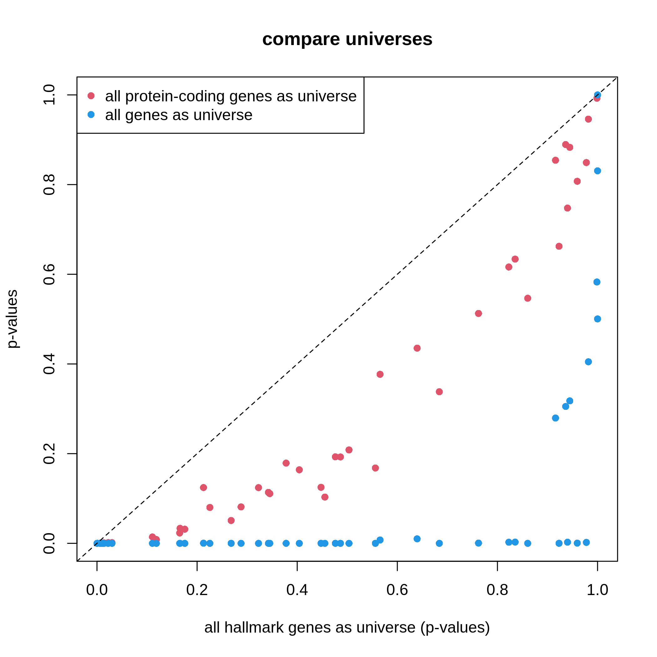
It is very straightforward to see, with a larger universe, there are more significant gene sets, which may produce potentially more false positives. This is definitely worse when using all genes in the genome as universe.
Based on the discussion in this section, the recommendation of using universe is:
- using protein-coding genes,
- using measured genes,
- or using a conservative way with clusterProfiler.
Visualization
clusterProfiler provides a rich set of visualization methods on the GSEA results, from simple visualization to complex ones. Complex visualizations are normally visually fancy but do not transfer too much useful information, and they should only be applied in very specific scenarios under very specific settings; while simple graphs normally do better jobs. Recently the visualization code in clusterProfiler has been moved to a new package enrichplot. Let’s first load the enrichplot package. The full sets of visualizations that enrichplot supports can be found from https://yulab-smu.top/biomedical-knowledge-mining-book/enrichplot.html.
We first re-generate the enrichment table.
R
library(enrichplot)
resTimeGO = enrichGO(gene = timeDEgenes,
                     keyType = "SYMBOL",
                     ont = "BP",
                     OrgDb = org.Mm.eg.db,
                     pvalueCutoff = 1,
                     qvalueCutoff = 1)
resTimeGOTable = as.data.frame(resTimeGO)
head(resTimeGOTable)
OUTPUT
                   ID                Description GeneRatio   BgRatio RichFactor
GO:0050900 GO:0050900        leukocyte migration    54/946 412/25615  0.1310680
GO:0006935 GO:0006935                 chemotaxis    56/946 476/25615  0.1176471
GO:0042330 GO:0042330                      taxis    56/946 478/25615  0.1171548
GO:0030595 GO:0030595       leukocyte chemotaxis    37/946 233/25615  0.1587983
GO:0060326 GO:0060326            cell chemotaxis    43/946 330/25615  0.1303030
GO:0071674 GO:0071674 mononuclear cell migration    34/946 229/25615  0.1484716
           FoldEnrichment    zScore       pvalue     p.adjust       qvalue
GO:0050900       3.548949 10.213913 6.488865e-16 3.281419e-12 9.099632e-13
GO:0006935       3.185549  9.425373 2.121016e-14 4.276849e-11 1.186004e-11
GO:0042330       3.172220  9.387925 2.537186e-14 4.276849e-11 1.186004e-11
GO:0030595       4.299808  9.908597 6.859406e-14 8.672004e-11 2.404815e-11
GO:0060326       3.528237  9.052150 7.528704e-13 7.614531e-10 2.111569e-10
GO:0071674       4.020191  8.990078 4.993702e-12 3.786134e-09 1.049925e-09
                                                                                                                                                                                                                                                                                                                                         geneID
GO:0050900                   Ccr7/Ccl2/Ptn/Prex1/Edn3/Itga4/Padi2/Emp2/Fpr2/Ccl5/S100a8/Sell/Cxcl1/Cd209a/Mdk/Ccl28/Hsd3b7/Ptk2b/S100a9/Lgals3/Tnfsf18/Dusp1/Il33/Nbl1/Itgb3/Trpm4/Retnlg/Itgam/Ppbp/Ccl7/C3/Aire/Alox5/Fut7/Ada/Aoc3/Calr/Pf4/Slamf9/Plg/Adam8/Bst1/Il12a/P2ry12/Grem1/Ascl2/AI182371/Cxcl5/Ch25h/Apod/Gdf15/Ager/Enpp1/Axdnd1
GO:0006935 Ccr7/Ccl2/Ptn/S100a7a/Prex1/Edn3/Padi2/Lsp1/Nr4a1/Fpr2/Ccl5/S100a8/Sell/Cxcl1/Mdk/Cmtm5/Ccl28/Hsd3b7/Ptk2b/S100a9/Cmtm7/Lgals3/Plxnb3/Tnfsf18/Dusp1/Nbl1/Itgb3/Trpm4/Retnlg/Itgam/Ppbp/Ccl7/Casr/Tubb2b/C3/Robo3/Alox5/Stx3/Ccl6/Lpar1/Calr/Nox1/Ptgr1/Pf4/Slamf9/Ntf3/Adam8/Bst1/Il12a/P2ry12/Grem1/AI182371/Cxcl5/Ch25h/Ccl17/Ager
GO:0042330 Ccr7/Ccl2/Ptn/S100a7a/Prex1/Edn3/Padi2/Lsp1/Nr4a1/Fpr2/Ccl5/S100a8/Sell/Cxcl1/Mdk/Cmtm5/Ccl28/Hsd3b7/Ptk2b/S100a9/Cmtm7/Lgals3/Plxnb3/Tnfsf18/Dusp1/Nbl1/Itgb3/Trpm4/Retnlg/Itgam/Ppbp/Ccl7/Casr/Tubb2b/C3/Robo3/Alox5/Stx3/Ccl6/Lpar1/Calr/Nox1/Ptgr1/Pf4/Slamf9/Ntf3/Adam8/Bst1/Il12a/P2ry12/Grem1/AI182371/Cxcl5/Ch25h/Ccl17/Ager
GO:0030595                                                                                                                 Ccr7/Ccl2/Ptn/Prex1/Edn3/Padi2/Fpr2/Ccl5/S100a8/Sell/Cxcl1/Mdk/Ccl28/Hsd3b7/Ptk2b/S100a9/Lgals3/Tnfsf18/Dusp1/Nbl1/Trpm4/Retnlg/Itgam/Ppbp/Ccl7/C3/Alox5/Calr/Pf4/Slamf9/Adam8/Bst1/Il12a/Grem1/AI182371/Cxcl5/Ch25h
GO:0060326                                                                              Ccr7/Ccl2/Ptn/Prex1/Edn3/Padi2/Nr4a1/Fpr2/Ccl5/S100a8/Sell/Cxcl1/Mdk/Ccl28/Hsd3b7/Ptk2b/S100a9/Lgals3/Plxnb3/Tnfsf18/Dusp1/Nbl1/Trpm4/Retnlg/Itgam/Ppbp/Ccl7/C3/Alox5/Ccl6/Lpar1/Calr/Nox1/Pf4/Slamf9/Adam8/Bst1/Il12a/Grem1/AI182371/Cxcl5/Ch25h/Ccl17
GO:0071674                                                                                                                              Ccr7/Ccl2/Itga4/Padi2/Fpr2/Ccl5/Cd209a/Mdk/Hsd3b7/Ptk2b/Lgals3/Tnfsf18/Dusp1/Nbl1/Itgb3/Trpm4/Retnlg/Ccl7/Aire/Alox5/Fut7/Calr/Slamf9/Plg/Adam8/Il12a/P2ry12/Grem1/Ascl2/AI182371/Ch25h/Apod/Ager/Enpp1
           Count
GO:0050900    54
GO:0006935    56
GO:0042330    56
GO:0030595    37
GO:0060326    43
GO:0071674    34
barplot() and dotplot() generate plots for
a small number of significant gene sets. Note the two functions are
directly applied on resTimeGO returned by
enrichGO().
R
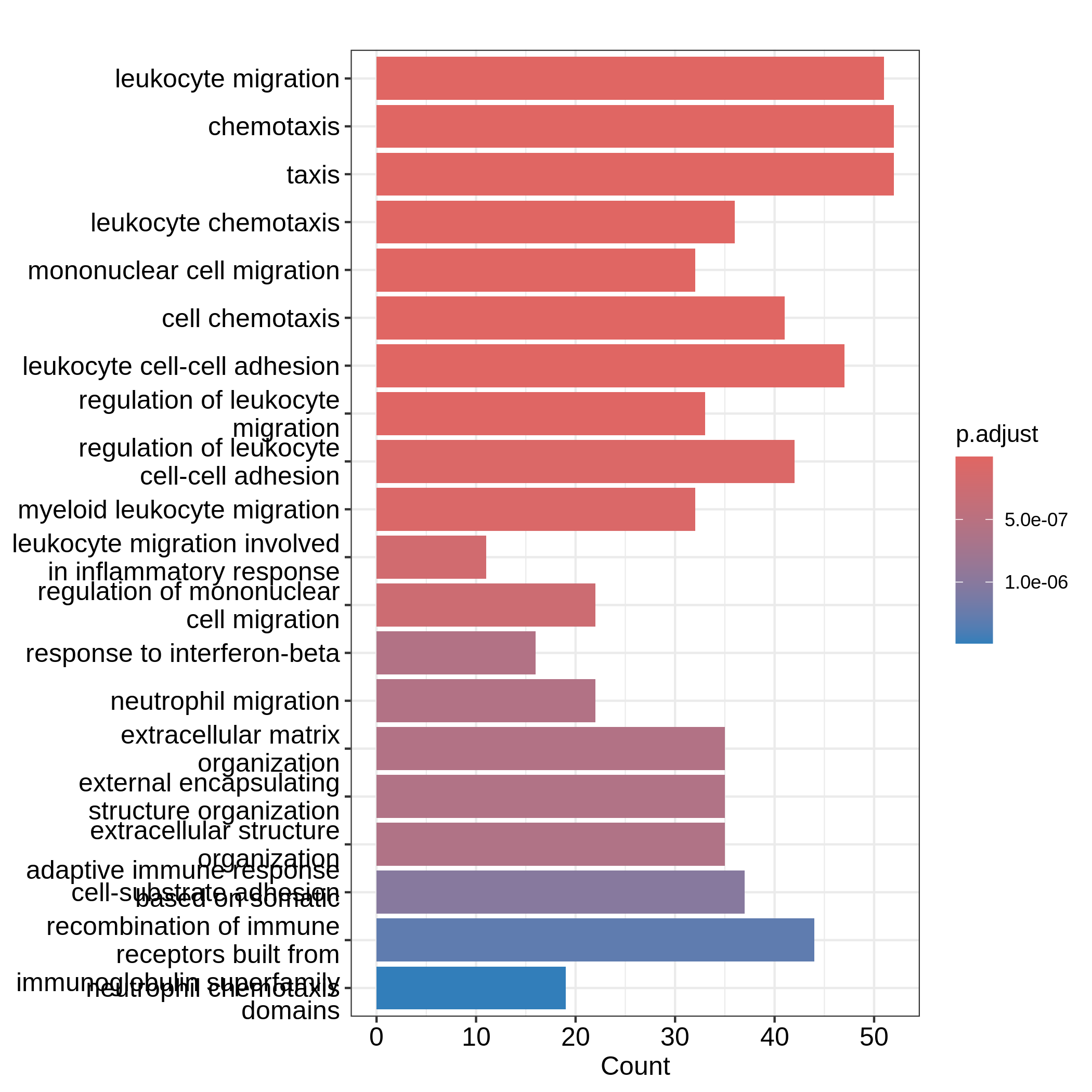
barplot(resTimeGO, showCategory = 20)
R
dotplot(resTimeGO, showCategory = 20)
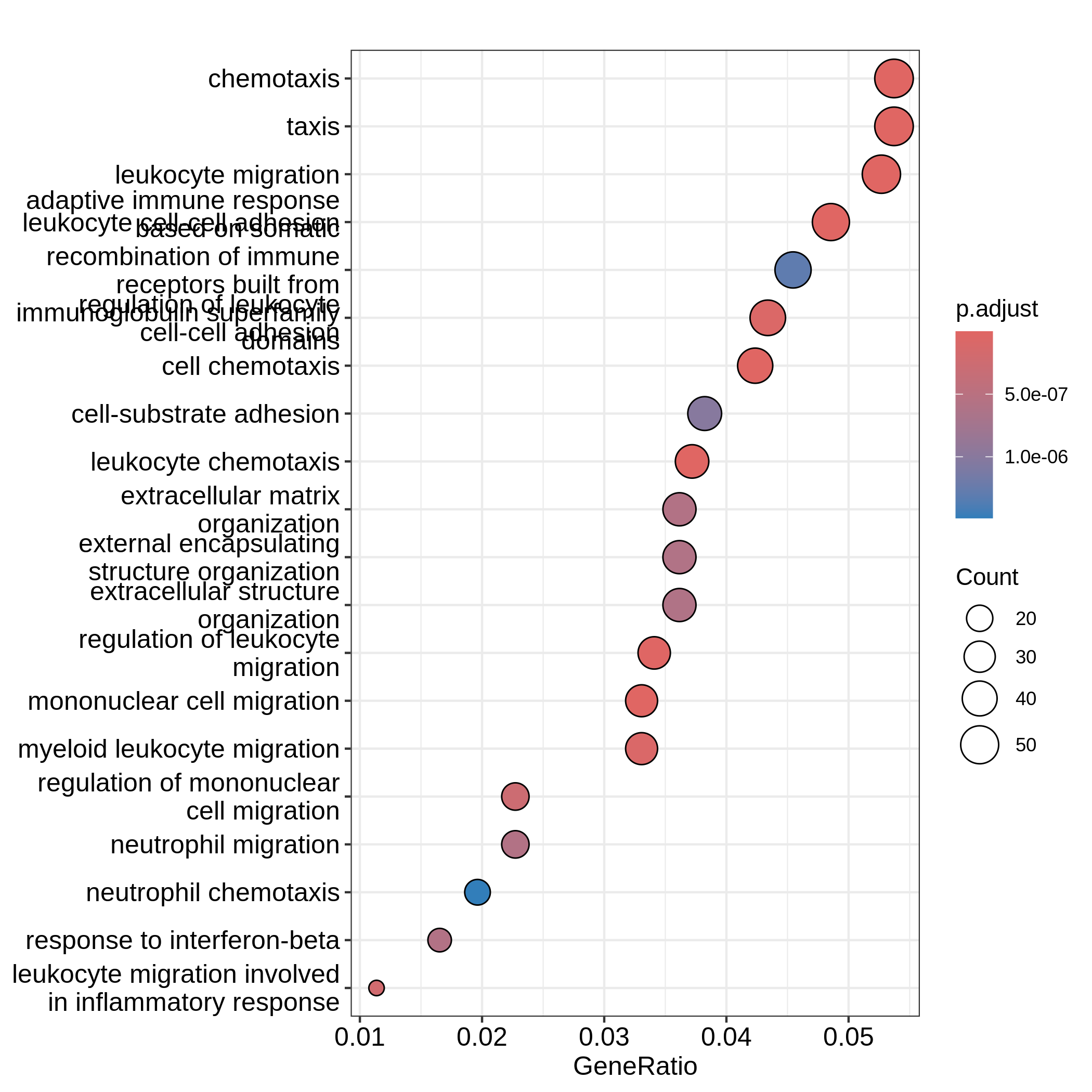
Barplots can map two variables to the plot, one to the height of bars
and the other to the colors of bars; while for dotplot, sizes of dots
can be mapped to a third variable. The variable names are in the colum
names of the result table. Both plots include the top 20 most
significant terms. On dotplot, terms are ordered by the values on x-axis
(the GeneRatio).
Now we need to talk about “what is a good visualization?”. The
essential two questions are “what is the key message a plot
transfers to readers?” and “what is the major graphical element
in the plot?”. In the barplot or dotplot, the major graphical
element which readers may notice the easiest is the height of bars or
the offset of dots to the origin. The most important message of the ORA
analysis is of course “the enrichment”. The two examples from
barplot() and dotplot() actually fail to
transfer such information to readers. In the first barplot where
"Count" is used as values on x-axis, the numer of DE genes
in gene sets is not a good measure of the enrichment because it has a
positive relation to the size of gene sets. A high value of
"Count" does not mean the gene set is more enriched.
It is the same reason for dotplot where "GeneRatio" is
used as values on x-axis. Gene ratio is calculated as the fraction of DE
genes from a certain gene set (GeneRatio = Count/Total_DE_Genes). The
dotplot puts multiple gene sets in the same plot and the aim is to
compare between gene sets, thus gene sets should be “scaled” to make
them comparable. "GeneRatio" is not scaled for different
gene sets and it still has a positive relation to the gene set size,
which can be observed in the dotplot where higher the gene ratio, larger
the dot size. Actually “GeneRatio” has the same effect as “Count”
(GeneRatio = Count/Total_DE_Genes), so as has been explained in the
previous paragraph, "GeneRatio" is not a good measure for
enrichment either.
Now let’s try to make a more reasonable barplot and dotplot to show the enrichment of ORA.
First, let’s define some metrics which measure the “enrichment” of DE genes on gene sets. Recall the denotations in the 2x2 contingency table (we are too far from that!). Let’s take these numbers from the enrichment table.
R
n_11 = resTimeGOTable$Count
n_10 = 983  # length(intersect(resTimeGO@gene, resTimeGO@universe))
n_01 = as.numeric(gsub("/.*$", "", resTimeGOTable$BgRatio))
n = 28943  # length(resTimeGO@universe)
Instead of using GeneRatio, we use the fraction of DE
genes in the gene sets which are kind of like a “scaled” value for all
gene sets. Let’s calculate it:
R
resTimeGOTable$DE_Ratio = n_11/n_01
resTimeGOTable$GS_size = n_01  # size of gene sets
Then intuitively, if a gene set has a higher DE_Ratio
value, we could say DE genes have a higher enrichment6 in it.
We can measure the enrichment in two other ways. First, the log2 fold enrichment, defined as:
\[ \log_2(\mathrm{Fold\_enrichment}) = \frac{n_{11}/n_{10}}{n_{01}/n} = \frac{n_{11}/n_{01}}{n_{10}/n} = \frac{n_{11}n}{n_{10}n_{01}} \]
which is the log2 of the ratio of DE% in the gene set and DE% in the universe or the log2 of the ratio of gene_set% in the DE genes and gene_set% in the universe. The two are identical.
R
resTimeGOTable$log2_Enrichment = log( (n_11/n_10)/(n_01/n) )
Second, it is also common to use z-score which is
\[ z = \frac{n_{11} - \mu}{\sigma} \]
where \(\mu\) and \(\sigma\) are the mean and standard deviation of the hypergeometric distribution. They can be calculated as:
R
hyper_mean = n_01*n_10/n

n_02 = n - n_01
n_20 = n - n_10
hyper_var = n_01*n_10/n * n_20*n_02/n/(n-1)
resTimeGOTable$zScore = (n_11 - hyper_mean)/sqrt(hyper_var)
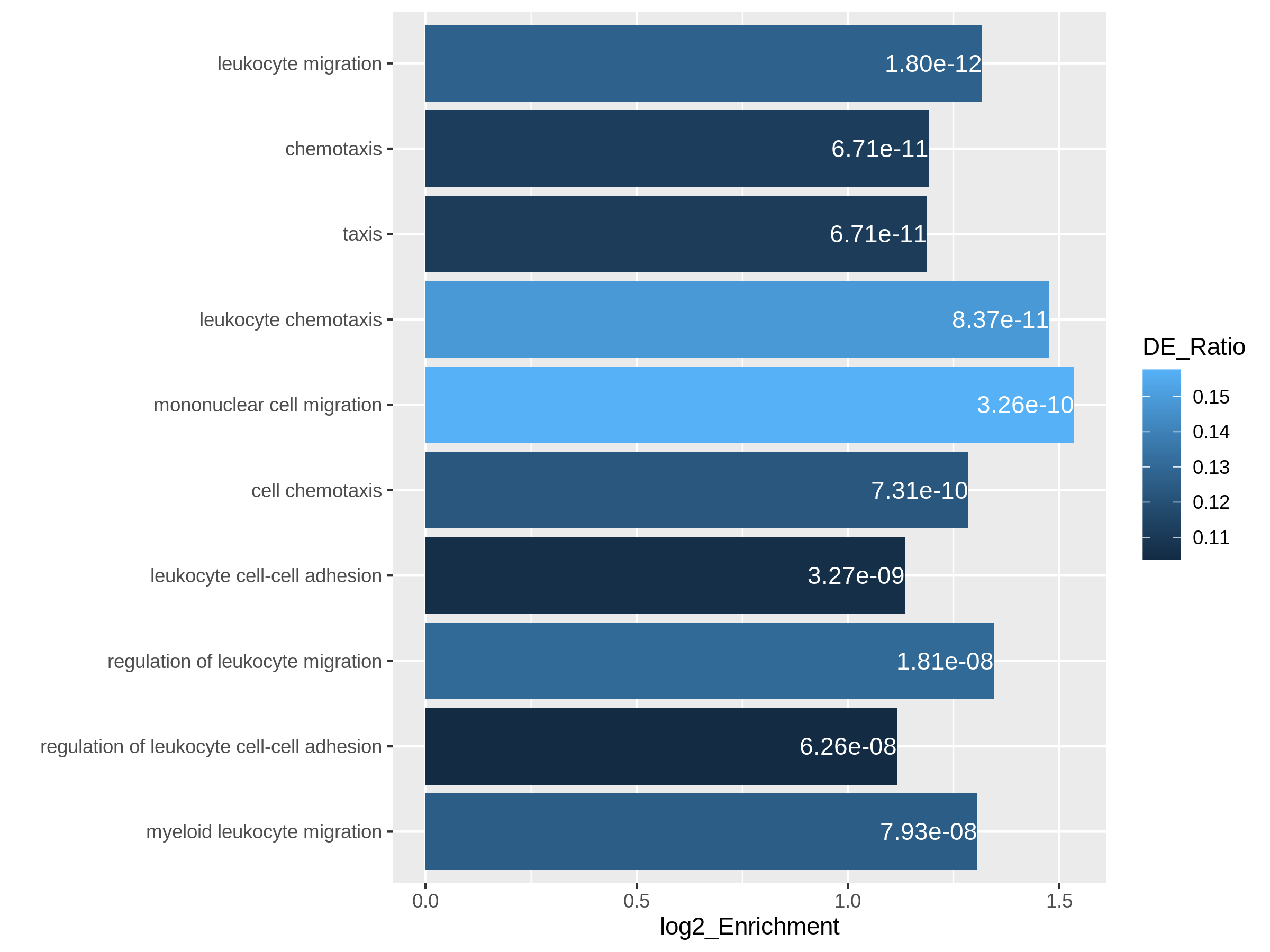
We will use log2 fold change as the primary variable to map to bar
heights and DE_Ratio as the secondary variable to map to
colors. This can be done directly with the ggplot2
package. We also add the adjusted p-values as labels on the
bars.
In resTimeGOTable, gene sets are already ordered by the
significance, so we take the first 10 gene sets which are the 10 most
significant gene sets.
R
library(ggplot2)
ggplot(resTimeGOTable[1:10, ],
        aes(x = log2_Enrichment, y = factor(Description, levels = rev(Description)),
            fill = DE_Ratio)) +
    geom_bar(stat = "identity") +
    geom_text(aes(x = log2_Enrichment,
        label = sprintf("%.2e", p.adjust)), hjust = 1, col = "white") +
    ylab("")
In the next example, we use z-score as the primary variable
to map to the offset to origin, DE_Ratio and
Count to map to dot colors and sizes.
R
ggplot(resTimeGOTable[1:10, ],
        aes(x = zScore, y = factor(Description, levels = rev(Description)),
            col = DE_Ratio, size = Count)) +
    geom_point() +
    ylab("")
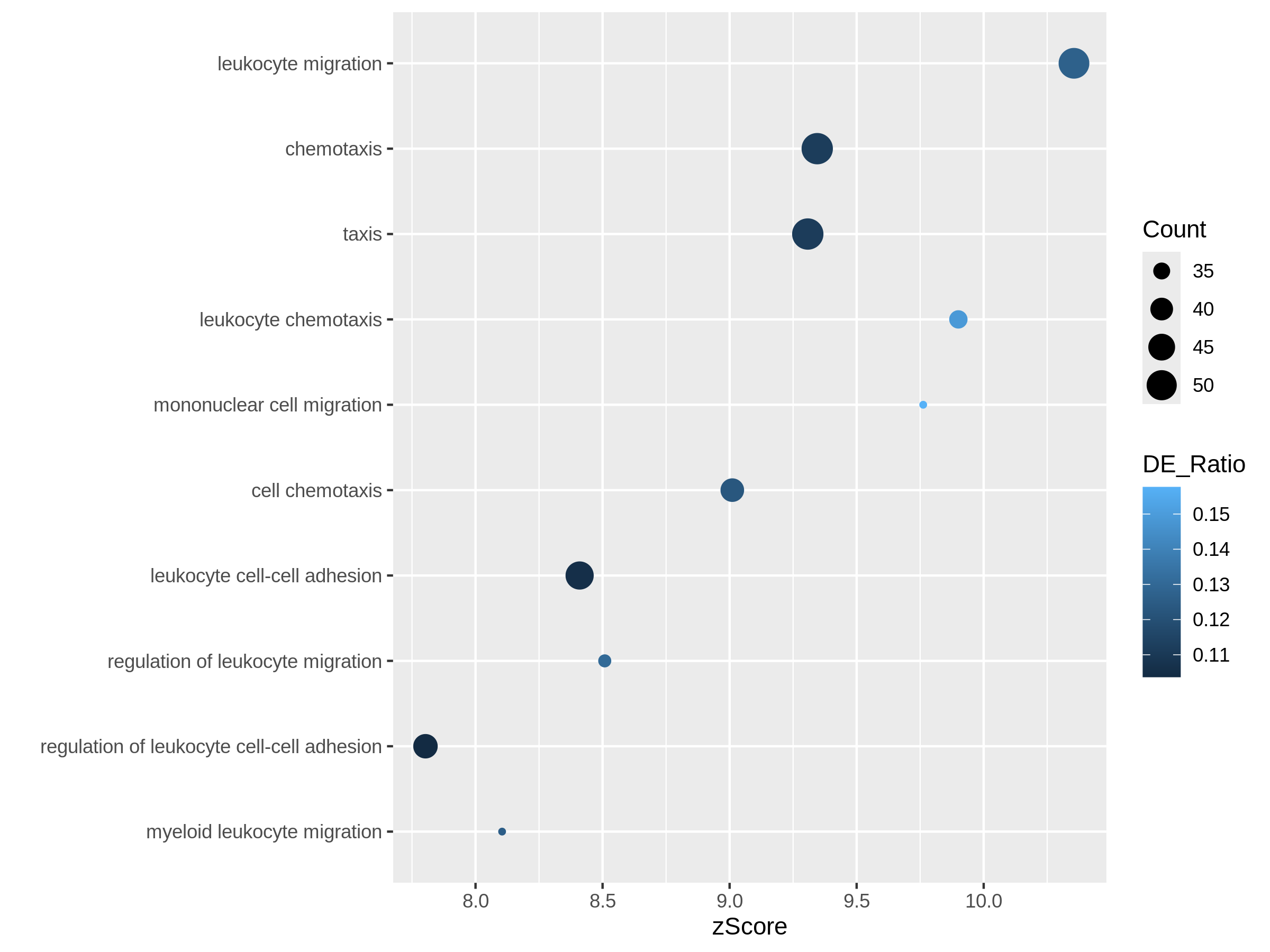
Both plots can highlight the gene set “leukocyte migration involved in inflammatory response” is relatively small but highly enriched.
Another useful visualization is the volcano plot. You may be aware of in differential expression analysis, in the volcano plot, x-axis corresponds to log2 fold changes of the differential expression, and y-axis corresponds to the adjusted p-values. It is actually similar here where we use log2 fold enrichment on x-axis.
Since we only look at the over-representation, the volcano plot is one-sided. We can set two cutoffs on the log2 fold enrichment and adjusted p-values, then the gene sets on the top right region can be thought as being both statistically significant and also biologically sensible.
R
ggplot(resTimeGOTable,
    aes(x = log2_Enrichment, y = -log10(p.adjust),
        color = DE_Ratio, size = GS_size)) +
    geom_point() +
    geom_hline(yintercept = -log10(0.01), lty = 2, col = "#444444") +
    geom_vline(xintercept = 1.5, lty = 2, col = "#444444")
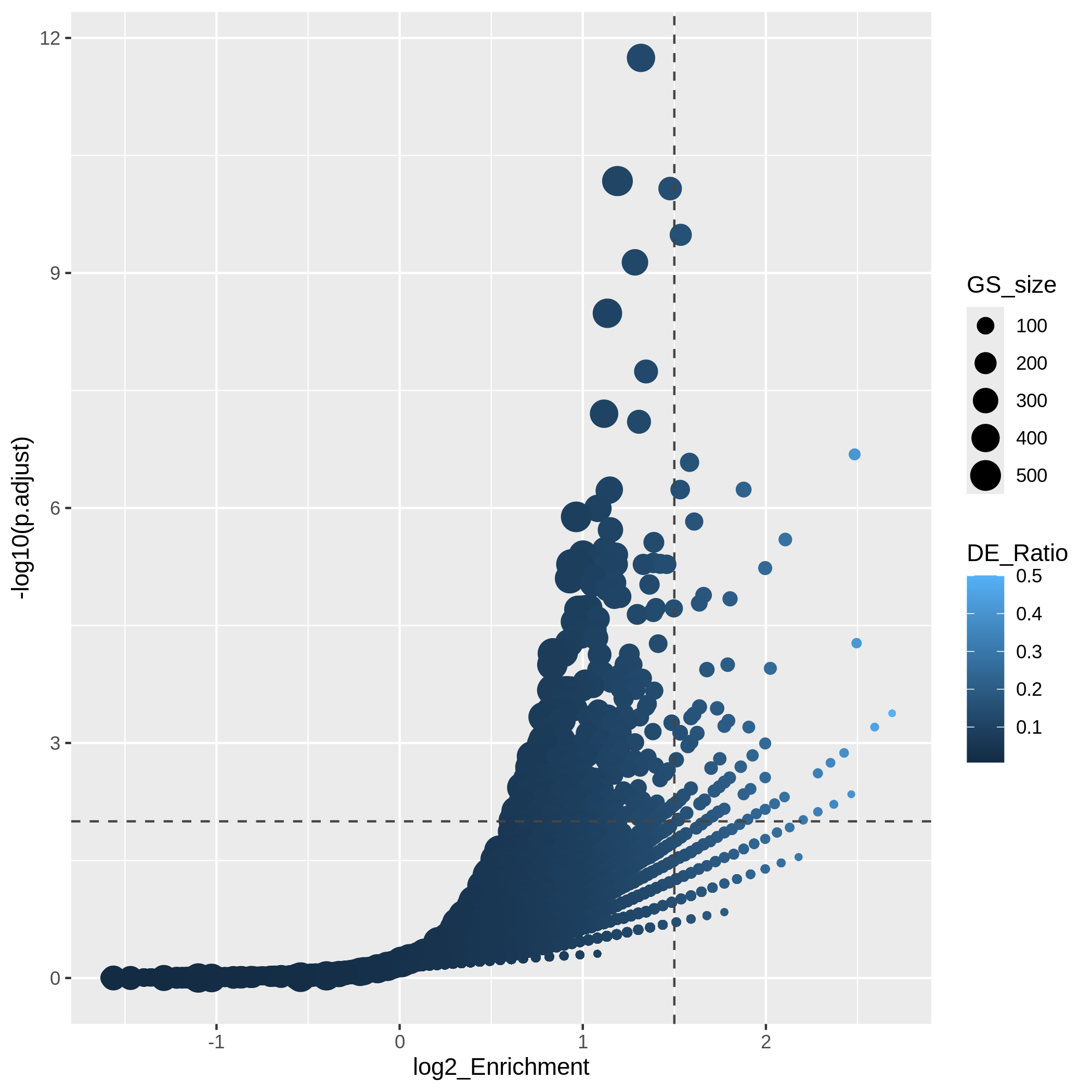
In the “volcano plot”, we can observe the plot is composed by a list
of curves. The trends are especially clear in the right bottom of the
plot. Actually each “curve” corresponds to a same "Count"
value (number of DE genes in a gene set). The volcano plot shows very
clearly that the enrichment has a positive relation to the gene set size
where a large gene set can easily reach a small p-value with a
small DE_ratio and a small log2 fold enrichment, while a small gene set
needs to have a large DE ratio to be significant.
It is also common that we perform ORA analysis on up-regulated genes and down-regulated separately. And we want to combine the significant gene sets from the two ORA analysis in one plot. In the following code, we first generate two enrichment tables for up-regulated genes and down-regulated separately.
R
# up-regulated genes
timeDEup <- as.data.frame(subset(resTime, padj < 0.05 & log2FoldChange > log2(1.5)))
timeDEupGenes <- rownames(timeDEup)

resTimeGOup = enrichGO(gene = timeDEupGenes,
                       keyType = "SYMBOL",
                       ont = "BP",
                       OrgDb = org.Mm.eg.db,
                       universe = rownames(se),
                       pvalueCutoff = 1,
                       qvalueCutoff = 1)
resTimeGOupTable = as.data.frame(resTimeGOup)
n_11 = resTimeGOupTable$Count
n_10 = length(intersect(resTimeGOup@gene, resTimeGOup@universe))
n_01 = as.numeric(gsub("/.*$", "", resTimeGOupTable$BgRatio))
n = length(resTimeGOup@universe)
resTimeGOupTable$log2_Enrichment = log( (n_11/n_10)/(n_01/n) )

# down-regulated genes
timeDEdown <- as.data.frame(subset(resTime, padj < 0.05 & log2FoldChange < -log2(1.5)))
timeDEdownGenes <- rownames(timeDEdown)

resTimeGOdown = enrichGO(gene = timeDEdownGenes,
                       keyType = "SYMBOL",
                       ont = "BP",
                       OrgDb = org.Mm.eg.db,
                       universe = rownames(se),
                       pvalueCutoff = 1,
                       qvalueCutoff = 1)
resTimeGOdownTable = as.data.frame(resTimeGOdown)
n_11 = resTimeGOdownTable$Count
n_10 = length(intersect(resTimeGOdown@gene, resTimeGOdown@universe))
n_01 = as.numeric(gsub("/.*$", "", resTimeGOdownTable$BgRatio))
n = length(resTimeGOdown@universe)
resTimeGOdownTable$log2_Enrichment = log( (n_11/n_10)/(n_01/n) )
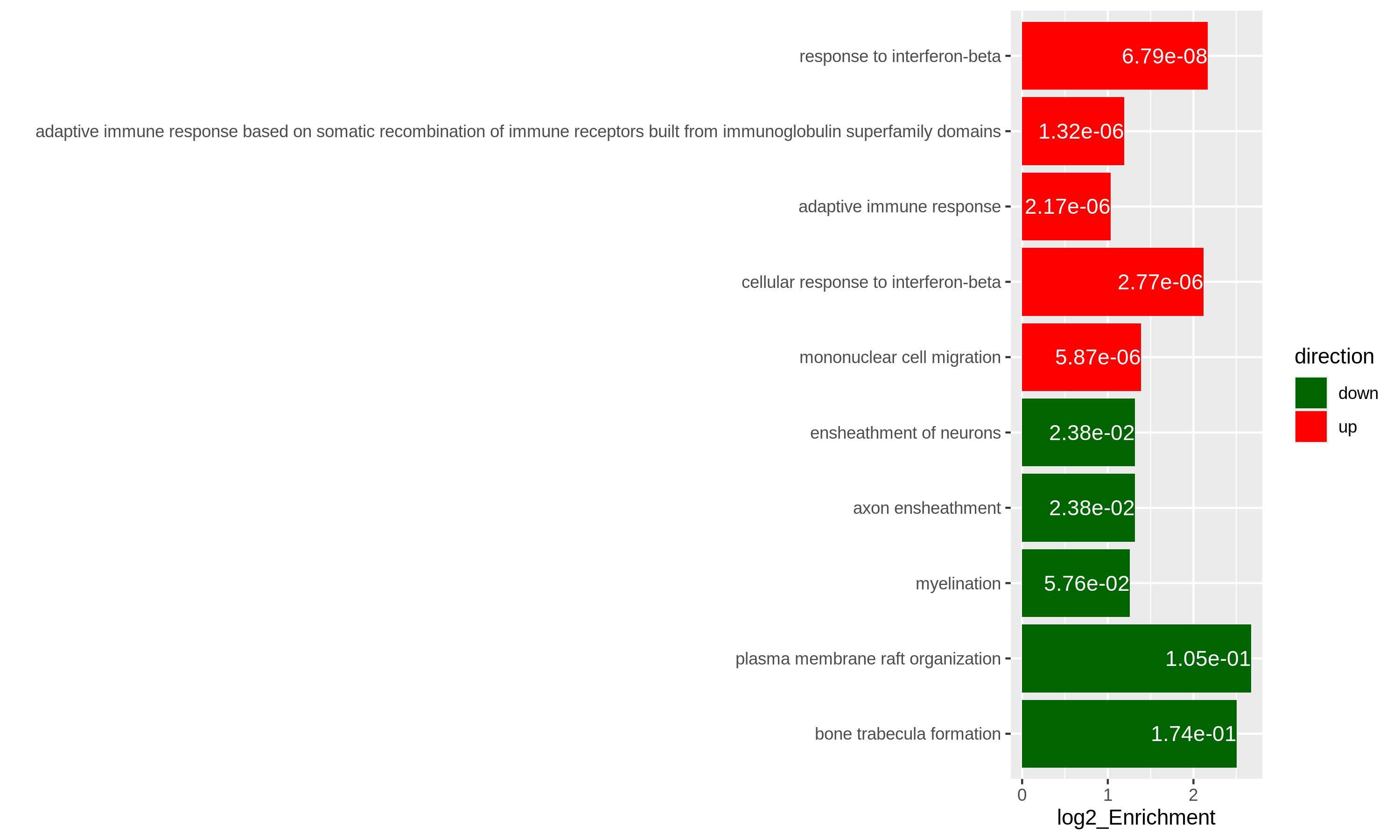
As an example, let’s simply take the first 5 most significant terms for up-regulated genes and the first 5 most significant terms for down-regulated genes. The following ggplot2 code should be easy to read.
R
# The name of the 3rd term is too long, we wrap it into two lines.
resTimeGOupTable[3, "Description"] = paste(strwrap(resTimeGOupTable[3, "Description"]), collapse = "\n")

direction = c(rep("up", 5), rep("down", 5))
ggplot(rbind(resTimeGOupTable[1:5, ],
             resTimeGOdownTable[1:5, ]),
        aes(x = log2_Enrichment, y = factor(Description, levels = rev(Description)),
            fill = direction)) +
    geom_bar(stat = "identity") +
    scale_fill_manual(values = c("up" = "red", "down" = "darkgreen")) +
    geom_text(aes(x = log2_Enrichment,
        label = sprintf("%.2e", p.adjust)), hjust = 1, col = "white") +
    ylab("")
Specifically for GO enrichment, it is often that GO enrichment returns a long list of significant GO terms (e.g. several hundreds). This makes it difficult to summarize the common functions from the long list. The last package we will introduce is the simplifyEnrichment package which partitions GO terms into clusters based on their semantic similarity7 and summarizes their common functions via word clouds.
The input of the simplifyGO() function is a vector of GO
IDs. It is recommended to have at least 100 GO IDs for summarization and
visualization.
R
GO_ID = resTimeGOTable$ID[resTimeGOTable$p.adjust < 0.1]
library(simplifyEnrichment)
simplifyGO(GO_ID)
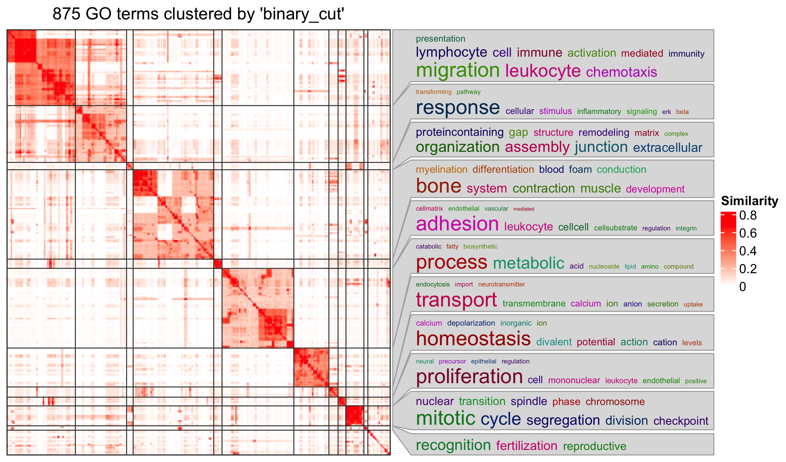
Further reading
ORA analysis actually applies a binary conversion on genes where genes pass the cutoff are set as 1 (DE gene) and others are set as 0 (non-DE gene). This binary transformation over-simplifies the problem and a lot of information are lost. There is second class of gene set enrichment analysis methods which takes the continuous gene-level score as input and weights the importance of a gene in the gene set. Please refer to Subramanian et. al. Gene set enrichment analysis: A knowledge-based approach for interpreting genome-wide expression profiles, PNAS 2005 for more information.
- ORA analysis is based on the gene counts and it is based on Fisher’s exact test or the hypergeometric distribution.
- In R, it is easy to obtain gene sets from a large number of sources.
Genes must be unique in each vector.↩︎
Also note
phyper()can be vectorized.↩︎The definition is from Wikipedia: https://en.wikipedia.org/wiki/Biological_pathway.↩︎
This is actually not true. Indeed
as.data.frame(resTimeGO)only returns the significant GO terms, but the complete enrichment table is still stored inresTimeGO@result. However, directly retrieving the slot of an S4 object is highly unrecommended.↩︎You can also use
select()function:select(org.Mm.eg.db, keys = timeDEgenes, keytype = "SYMBOL", column = "ENTREZID")↩︎If here the term “enrichment” does mean statistically.↩︎
The semantic similarity between GO terms considers the topological relations in the GO hierarchy.↩︎