Content from What is a reprex and why is it useful?

Last updated on 2025-08-26 | Edit this page

Overview

Questions

What steps can you take to solve problems in your code?
What is a minimal reproducible example?
Why are minimal reproducible examples important?
What is the Portal Project dataset?

Objectives

Describe a minimal reproducible example and its requirements.
Recognize how creating a minimal reproducible example can help you solve problems in your code.
List the key steps to creating a minimal reproducible example.
Explain the benefits of creating a minimal reproducible example both for you and for others.
Load in the rodent survey data and briefly explain its contents.

One of the most frustrating parts of learning to code is getting stuck and not knowing what to do! Maybe R gives you an angry red error message you don’t understand, or your code doesn’t seem to be doing what you were expecting and you don’t know why. Maybe you try to use Google to find answers but you can’t quite find the same problem out there. What to do?

Luckily, there are many people in the R and data science communities who are happy to help. However, in order for them to do so, you must give them the right information. Figuring out how to ask a good question can be hard.

Many helpers or forums may ask you to provide example data or a minimal reproducible example (commonly abbreviated as a “reprex”). What even is that? Wouldn’t it be nice if you could just hand over your computer so a helper can see exactly what is happening? That’s exactly what the reprex is for.

What is a reprex?

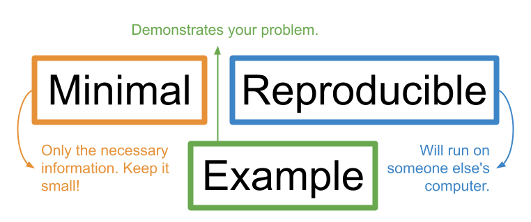
A reprex is essentially a simplified version of your problematic code that clearly demonstrates the problem you are facing (includes only the necessary information to show the problem, nothing more) and will run easily on anyone’s computer.

The Tidyverse documentation puts it simply:

“The goal of a reprex is to package your problematic code in such a way that other people can run it and feel your pain. Then, hopefully, they can provide a solution and put you out of your misery.” - Get help! (Tidyverse)

Why use a reprex?

Reprexes are very important tools to get help when you’re stuck on a coding problem. You may be asked to provide a reprex when you’re working with a statistical consultant (often available at universities) or when posting a question to online help forums (such as StackOverflow or the Posit Community).

As the name suggests, a minimal reproducible example needs to be minimal and reproducible.

Stripping the code and data down to their essential (minimal) parts makes it easy for a helper to zero-in on what might be going wrong.
Making your example reproducible allows a helper to run your code on their own computer so they can easily “tinker” with it to fix it. This makes them more likely to help you.

Callout

Helpers

There are lots of people who might help you with your code: friends, colleagues, mentors, or total strangers online. In this lesson, we will use the term “helper” to refer to the person who is helping you to debug your code. Helpers are the target audience for your minimal reproducible example.

But there’s another hidden reason to make a reprex! The process of making a reprex often leads to a better understanding of your own code. Therefore, you might end up solving the problem yourself without asking for help.

Callout

Rubber duck debugging

The phenomenon of solving one’s own problem during the process of trying to explain it to someone else is often called “rubber duck debugging.” This is a reference to a story about programmers who would explain the problem they were having with their code to a rubber duck they would keep on their desk. Jenny Bryan refers to reprexes as “basically the rubber duck in disguise,” because they force you to unpack your problem to explain it more clearly.

Jenny Bryan shares many other insights about reprexes in her 2018 talk “Help me help you: Creating reproducible examples.”

Making a reprex can be an excellent learning opportunity, but the process can feel daunting when you are not sure where to begin. In this lesson, we will walk through a step by step roadmap you can use whenever you feel stuck, including some first steps for debugging your code and the process of creating a reprex. We’ll talk about each of the steps and provide a workflow that you can follow when you get stuck in the future. At the end, we’ll introduce you to the {reprex} package, a useful tool for creating good minimal reproducible examples. By the end of the lesson you will have gained a better understanding of how to approach error and warning messages, you will feel more confident in your ability to make a reprex, and you will feel more comfortable asking for formal help.

Meet Mickey, your learning companion

Mickey is an ecology grad student who just joined a new lab. Mickey’s lab has been working for many years with data from the Portal Project, a long-term research study of rodents in Portal, Arizona. Mickey would like to explore this data for their research, so they reach out to Remy, a fifth-year grad student who is very familiar with this project. To get Mickey started, Remy sends Mickey an archival dataset of rodent surveys from 1977-1989, and tells Mickey to “play around” with the data in RStudio to get familiar with it.

Mickey has some past experience in R. They attended the “Data Analysis and Visualization in R for Ecologists” Carpentries workshop, and they feel comfortable with the fundamentals of coding in R. Still, Mickey is a little rusty and nervous about their skills and the unfamiliar data.

Callout

Prerequisites and target audience

This workshop assumes some prior experience with working in R and RStudio. We will assume you’ve taken the equivalent of the Data Analysis and Visualization in R for Ecologists workshop and are comfortable with basic commands, and we won’t necessarily explain every line of code in detail.

If you’re much more experienced in R, this workshop is still for you! Even expert coders may not always know how to get unstuck. We hope this workshop will be useful to people with a variety of coding backgrounds.

Mickey starts by loading the data so they can begin to explore it. They also load the {tidyverse}, a set of packages that will be useful for wrangling and visualizing the data.

Let’s go over to RStudio. Make sure that you’re in the RStudio project that you created for this lesson, and that you’ve downloaded the data as a csv and saved it in the “data/” folder.

Callout

As a reminder: Make sure you’re coding in your RStudio project. You can open the project you created by double-clicking the “.Rproj” file from your Finder/File Explorer. Or, from inside of RStudio, navigate to the upper right corner of the screen, click on the blue cube icon, choose “Open Project”, and then select your project to open a new session of RStudio.

Now, we can load in the dataset with the following code:

R

# Loading the tidyverse package
library(tidyverse)

R

# Uploading the dataset that is currently saved in the project's data folder
surveys <- read_csv("data/surveys_complete_77_89.csv")

OUTPUT

Rows: 16878 Columns: 13
── Column specification ────────────────────────────────────────────────────────
Delimiter: ","
chr (6): species_id, sex, genus, species, taxa, plot_type
dbl (7): record_id, month, day, year, plot_id, hindfoot_length, weight

ℹ Use `spec()` to retrieve the full column specification for this data.
ℹ Specify the column types or set `show_col_types = FALSE` to quiet this message.

Mickey loads in the dataset and takes a look at it to find out what type of data was collected during these surveys.

R

# Take a look at the data
glimpse(surveys)

# or you can use
str(surveys)

OUTPUT

Rows: 16,878
Columns: 13
$ record_id       <dbl> 1, 2, 3, 4, 5, 6, 7, 8, 9, 10, 11, 12, 13, 14, 15, 16,…
$ month           <dbl> 7, 7, 7, 7, 7, 7, 7, 7, 7, 7, 7, 7, 7, 7, 7, 7, 7, 7, …
$ day             <dbl> 16, 16, 16, 16, 16, 16, 16, 16, 16, 16, 16, 16, 16, 16…
$ year            <dbl> 1977, 1977, 1977, 1977, 1977, 1977, 1977, 1977, 1977, …
$ plot_id         <dbl> 2, 3, 2, 7, 3, 1, 2, 1, 1, 6, 5, 7, 3, 8, 6, 4, 3, 2, …
$ species_id      <chr> "NL", "NL", "DM", "DM", "DM", "PF", "PE", "DM", "DM", …
$ sex             <chr> "M", "M", "F", "M", "M", "M", "F", "M", "F", "F", "F",…
$ hindfoot_length <dbl> 32, 33, 37, 36, 35, 14, NA, 37, 34, 20, 53, 38, 35, NA…
$ weight          <dbl> NA, NA, NA, NA, NA, NA, NA, NA, NA, NA, NA, NA, NA, NA…
$ genus           <chr> "Neotoma", "Neotoma", "Dipodomys", "Dipodomys", "Dipod…
$ species         <chr> "albigula", "albigula", "merriami", "merriami", "merri…
$ taxa            <chr> "Rodent", "Rodent", "Rodent", "Rodent", "Rodent", "Rod…
$ plot_type       <chr> "Control", "Long-term Krat Exclosure", "Control", "Rod…
spc_tbl_ [16,878 × 13] (S3: spec_tbl_df/tbl_df/tbl/data.frame)
 $ record_id      : num [1:16878] 1 2 3 4 5 6 7 8 9 10 ...
 $ month          : num [1:16878] 7 7 7 7 7 7 7 7 7 7 ...
 $ day            : num [1:16878] 16 16 16 16 16 16 16 16 16 16 ...
 $ year           : num [1:16878] 1977 1977 1977 1977 1977 ...
 $ plot_id        : num [1:16878] 2 3 2 7 3 1 2 1 1 6 ...
 $ species_id     : chr [1:16878] "NL" "NL" "DM" "DM" ...
 $ sex            : chr [1:16878] "M" "M" "F" "M" ...
 $ hindfoot_length: num [1:16878] 32 33 37 36 35 14 NA 37 34 20 ...
 $ weight         : num [1:16878] NA NA NA NA NA NA NA NA NA NA ...
 $ genus          : chr [1:16878] "Neotoma" "Neotoma" "Dipodomys" "Dipodomys" ...
 $ species        : chr [1:16878] "albigula" "albigula" "merriami" "merriami" ...
 $ taxa           : chr [1:16878] "Rodent" "Rodent" "Rodent" "Rodent" ...
 $ plot_type      : chr [1:16878] "Control" "Long-term Krat Exclosure" "Control" "Rodent Exclosure" ...
 - attr(*, "spec")=
  .. cols(
  ..   record_id = col_double(),
  ..   month = col_double(),
  ..   day = col_double(),
  ..   year = col_double(),
  ..   plot_id = col_double(),
  ..   species_id = col_character(),
  ..   sex = col_character(),
  ..   hindfoot_length = col_double(),
  ..   weight = col_double(),
  ..   genus = col_character(),
  ..   species = col_character(),
  ..   taxa = col_character(),
  ..   plot_type = col_character()
  .. )
 - attr(*, "problems")=<externalptr>

Looking over Mickey’s shoulder, Remy explains that the dataset is made up of many individual rodent records (record_id). The date of each record is given by the month, day, and year columns.

The dataset includes data from a number of different study plots that had different treatments applied: plot IDs are given by the plot_id column, and the type of treatment is specified in plot_type.

There is information about the genus and species of each individual caught. There is a species_id column that identifies the species of each individual caught.

In addition, there is a column called taxa that contains higher-level taxonomic information. Most of the observations are rodents, but there are also some birds, rabbits, and reptiles.

R

table(surveys$taxa)

OUTPUT


   Bird  Rabbit Reptile  Rodent
    300      69       4   16148

For each individual caught, the field crew took weight, sex and hindfoot_length measurements when possible, so values are sometimes missing.

Overall, the dataset contains 16,878 rodent observations ranging across years from 1977 through 1989.

With a clear understanding of the data, Mickey is now free to explore on their own. However, Remy notices that Mickey still looks nervous and decides to share a tool they recently found useful: a roadmap to getting unstuck in R by making a reprex.

Remy’s roadmap outlines four key steps for making a reprex. It is also intended to help the user better understand their problem and potentially find a solution along the way. Remy follows these steps any time they get stuck while coding. Indeed, the first portion of the roadmap, which Remy likes to call “code first aid,” includes preliminary steps to help identify and diagnose the problem, such as determining the type of error, reading function documentation, interpreting error messages, and running through the code line by line.

Remy explains that sometimes, these first aid steps are enough to solve code problems. But if not, the rest of the roadmap will lead Mickey through strategies to better understand the problem and demonstrate it to others in a minimal reproducible example (“reprex”).

Remy emphasizes to Mickey that they are happy to keep helping, but they will be very busy trying to finish writing their dissertation. If Mickey can first follow the steps outlined in this roadmap, then Remy can more easily help with whatever Mickey is struggling to resolve.

With an introduction to the dataset and a roadmap to guide them if they get stuck, Mickey feels ready to start coding!

Key Points

Throughout this lesson, we will be walking through a “roadmap” to getting unstuck in R by creating a minimal reproducible example (“reprex”).
A reprex is a simplified version of your problematic code that clearly demonstrates the problem you are facing and will run on anyone’s computer.
A reprex should contain only the minimum required to replicate the problem from any device so that helpers can more easily tinker and debug your code.
The process of building a reprex helps you better understand your code, your data, and your problem so that you will often find the solution yourself!
The surveys dataset includes records of rodents captured in a variety of experimental plots over a 12-year period, including some data about each rodent’s sex and morphology.

Content from Identify the problem and make a plan

Last updated on 2025-08-26 | Edit this page

Overview

Questions

What do I do when I encounter an error?
What do I do when my code outputs something I don’t expect?
Why do errors and warnings appear in R?
How can I find which areas of code are responsible for errors?
How can I fix my code? What other options exist if I can’t fix it?

Objectives

After completing this episode, participants should be able to…

Describe how the desired code output differs from the actual output
Categorize an error message (e.g. syntax error, semantic errors, package-specific errors, etc.)
Describe what an error message is trying to communicate
Identify specific lines and/or functions generating the error message
Use R Documentation to look up function syntax and examples
Quickly fix commonly-encountered R errors using ‘code first aid’
Identify when a problem is better suited for asking for further help, including making a reprex

Let’s take a look in more detail at the first step of the roadmap.

In this episode, we’ll cover what to do when you first encounter an error or undesired output from your code. We’ll cover the basics of identifying errors, fixing them if possible, and determining when to create a reprex. At the end of the lesson, we’ll return to Mickey’s analysis.

The first step in solving a problem is understanding what is going wrong. Sometimes R will help you out by displaying an error message when it is unable to run your code. This is a helpful diagnostic tool that, when interpreted correctly, can quickly lead you to a solution. Other times, R doesn’t encounter any problems running your code, but the output is not what you expected. These problems may require a few extra steps to properly diagnose. We will start with easier scenarios and provide helpful “code first aid” steps as we build up to harder challenges.

Strategy 1: Interpret error messages and change function inputs

R will often let us know there’s a problem by displaying an error message. An error that generates an error message is called a syntax error. Error messages happen when R is not able to run your code (this is in contrast to a warning message, which gives a hint that something could be wrong while the code keeps running). Error messages are sometimes straightforward, but other times they can be very tricky to decipher. In this lesson, will teach some tools for interpreting syntax errors for yourself.

Here’s an example error message. In the last episode, we saw that the taxa column contains information about the higher-level taxon of each organism caught, such as “Rodent” or “Bird”. We decide to look at the distribution of taxa by creating a frequency table.

R

table(taxa)

ERROR

Error: object 'taxa' not found

This code produces an error. What’s going on?

R is telling us that it can’t find taxa in the local environment. That’s because we haven’t told it where to look–recall that taxa is the name of a column in the surveys dataset.

The information from the error message doesn’t specifically tell us how to solve the error, but it can help us realize what went wrong. In this case, we can look back at our previous code and see that we were able to point R to the column using the $ operator:

R

table(surveys$taxa)

OUTPUT


   Bird  Rabbit Reptile  Rodent
    300      69       4   16148

That’s better! Now, let’s make a barplot of this column to show this same information.

R

# Make a plot of the different taxa in the rodents dataset
ggplot(aes(x = surveys$taxa)) + geom_bar()

ERROR

Error in `fortify()`:
! `data` must be a <data.frame>, or an object coercible by `fortify()`,
  or a valid <data.frame>-like object coercible by `as.data.frame()`, not a
  <uneval> object.
ℹ Did you accidentally pass `aes()` to the `data` argument?

It seems like that should have worked, but we got another error message, and this one seems harder to interpret. Once again, let’s go over each part of the error message and see if it provides any clues.

First, we see an error from a function called fortify, which we didn’t even use! Then, there’s a more helpful informational message: “Did you accidentally pass aes() to the data argument?” This does seem to relate to our line of code, as we do pass aes into the ggplot function. But what is this “data argument?”

Strategy 2: Read function documentation

Reading the error message gave us some clues, but it wasn’t enough to fix the problem. Let’s try another strategy. Reading the function documentation can improve our understanding of how the function works, and often that can reveal problems with our code.

Let’s access the documentation for the function ggplot:

R

?ggplot

A Help window pops up in RStudio. [Add discussion of the different sections of function documentation, in general terms, here?] The “Usage” and “Arguments” sections tell us that ggplot takes the argument data, followed by mapping, which uses aes(). The “Arguments” section tells us that if the object passed to that first data argument isn’t already a data frame, ggplot will try to convert it to a data frame using fortify. That function, fortify, sounds familiar from the error message! This gives us an important clue. It looks like we accidentally passed the mapping argument into the position where ggplot expected data in the form of a data frame.

The “Examples” section of the function documentation can be particularly helpful because it shows how functions are used in context. The “Examples” section in the ggplot documentation, under “Pattern 1”, shows exactly how ggplot expects the data and mapping arguments to be written.

Using this information, we can change our code to put the arguments in the right order–first the name of the dataset for the data argument, and then the aes() call for the mapping argument.

R

ggplot(data = surveys, mapping = aes(x = taxa)) + geom_bar()

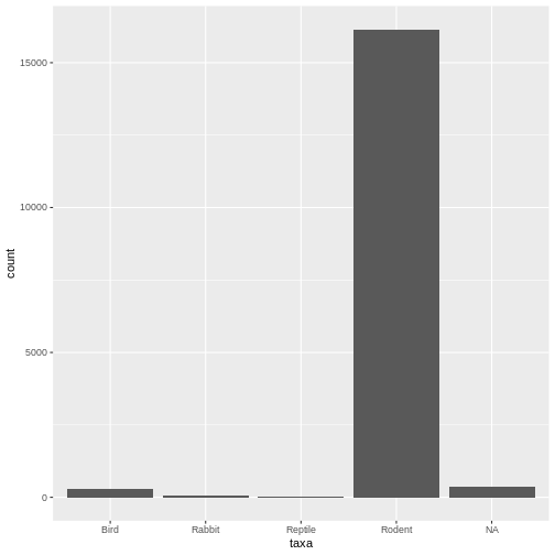
The error message is gone, and it works! Here we see our desired plot. What do you notice about the data?

- Lots of rodents - Some missing values (NAs)

Let’s take a moment to highlight some patterns we’re starting to see in the course of tinkering with our code.

First, we noticed a problem. In this case, the problem was a syntax error, in which the code failed to run and we got an error message.

We carefully read the error message and took a guess at what might be wrong. We changed the inputs to the function accordingly and tried again.

When we encountered another error message, we looked through the function documentation to find more clues about how to fix the error. This helped us see that we were missing an argument.

Another strategy we could have tried would be to copy and paste the error message into a search engine or a generative LLM for more interpretable explanations. And, when all else fails, we can prepare our code into a reproducible example for expert help.

Let’s see if we can use the strategies we’ve learned so far to address a new problem. Here they are, for reference:

Callout

Code first aid strategies

Interpret error messages and tweak inputs
Look at the function documentation
Put the error message into a search engine or a generative LLM

Challenge

Exercise 1: Applying code first aid

Below we see an error message pop up when trying to quantify the counts of genus and species in our dataset. Which of the following interpretations of the error message most aptly describes the problem (hint: look at the ?tally documentation if you’re stuck!)

R

surveys %>% tally(genus, species)

ERROR

Error in `tally()`:
ℹ In argument: `n = sum(genus, na.rm = TRUE)`.
Caused by error in `sum()`:
! invalid 'type' (character) of argument

tally does not accept 'type' (character) arguments. We should change genus and species to factors or numbers and run this line again.
tally does not accept 'type' (character) arguments. There is no way to quantify these data with this function.
tally does not accept 'type' (character) arguments. We need to assign a weight (e.g. 1) to each row so it knows how much to numerically weigh each observation.
tally does not accept 'type' (character) arguments. This function is not intended to group_by two variables and a different function (count) is required instead.

Show me the solution

d is the correct answer!

R

surveys %>% count(genus, species)

OUTPUT

# A tibble: 36 × 3
   genus            species             n
   <chr>            <chr>           <int>
 1 Ammospermophilus harrisi           136
 2 Amphispiza       bilineata         223
 3 Baiomys          taylori             3
 4 Calamospiza      melanocorys        13
 5 Callipepla       squamata           16
 6 Campylorhynchus  brunneicapillus    23
 7 Chaetodipus      penicillatus      382
 8 Crotalus         scutalatus          1
 9 Crotalus         viridis             1
10 Dipodomys        merriami         5675
# ℹ 26 more rows

Semantic errors

Let’s go back to our rodent analysis. We would like to subset the data to include only the Rodent taxon (as opposed to the other taxa included in the dataset: Bird, Rabbit, Reptile or NA). Let’s quickly check to see how much data we’d be throwing out by doing so:

R

table(surveys$taxa)

OUTPUT


   Bird  Rabbit Reptile  Rodent
    300      69       4   16148

We’re interested in the rodents, and thankfully it seems like a majority of our observations will be maintained when subsetting to rodents. But wait… In the barplot above, we could clearly see that there were some NA values. Why don’t we see them here?

This is a new type of problem, called a semantic error: the R code ran without any error messages, but it produced an unexpected output. Because there is no error message, semantic errors can be sneaky and hard to notice!

We can’t use our first code first aid strategy here, since there is no error message to read. So let’s jump straight to strategy 2, reading the function documentation.

R

?table

OUTPUT

Help on topic 'table' was found in the following packages:

  Package               Library
  vctrs                 /home/runner/.local/share/renv/cache/v5/linux-ubuntu-jammy/R-4.5/x86_64-pc-linux-gnu/vctrs/0.6.5/c03fa420630029418f7e6da3667aac4a
  base                  /home/runner/.cache/R/renv/sandbox/linux-ubuntu-jammy/R-4.5/x86_64-pc-linux-gnu/9a444a72


Using the first match ...

The documentation for table provides some clues. The “Usage” and “Arguments” sections show us an argument called useNA that accepts “no”, “ifany”, and “always”, but it’s not immediately apparent which one we should use to show our NA values. When we look at “Examples”, we find something else that looks helpful:

R

table(a)                 # does not report NA's
table(a, exclude = NULL) # reports NA's

Aha! So it looks like we can use exclude = NULL to report NAs in our table. Let’s try that.

R

table(surveys$taxa, exclude = NULL)

OUTPUT


   Bird  Rabbit Reptile  Rodent    <NA>
    300      69       4   16148     357

Problem solved! Now the NA values show up in the table. We see that by subsetting to the “Rodent” taxa, we would losing about 357 NAs, which themselves could be rodents! However, in this case, it seems a small enough portion to safely omit. Let’s subset our data to the rodent taxon.

R

# Just rodents
rodents <- surveys %>% filter(taxa == "Rodent")

Challenge

Exercise 2: Syntax vs. semantic errors

There are 3 lines of code below, and each attempts to create the same plot. Identify which produces a syntax error, which produces a semantic error, and which correctly creates the plot (hint: this may require you inferring what type of graph we’re trying to create!)

ggplot(rodents) + geom_bin_2d(aes(month, plot_type))
ggplot(rodents) + geom_tile(aes(month, plot_type), stat = "count")
ggplot(rodents) + geom_tile(aes(month, plot_type))

Show me the solution

In this case, A correctly creates the graph, plotting as colors in the tile the number of times an observation is seen. It essentially runs the following lines of code:

R

rodents_summary <- rodents %>% group_by(plot_type, month) %>% summarize(count=n())

OUTPUT

`summarise()` has grouped output by 'plot_type'. You can override using the
`.groups` argument.

R

ggplot(rodents_summary) + geom_tile(aes(month, plot_type, fill=count))

B is a syntax error, and will produce the following error:

R

ggplot(rodents) + geom_tile(aes(month, plot_type), stat = "count")

ERROR

Error in `geom_tile()`:
! Problem while computing stat.
ℹ Error occurred in the 1st layer.
Caused by error in `setup_params()`:
! `stat_count()` must only have an x or y aesthetic.

Finally, C is a semantic error. It does produce a plot, which is rather meaningless:

R

ggplot(rodents) + geom_tile(aes(month, plot_type))

The steps to identifying the problem and in code first aid matches what we’ve seen above. However, here seeing the problem arise in our code may be much more subtle, and comes from us recognizing output we don’t expect or know to be wrong. Even if the code is run, R may give us warning or informational messages which pop up when executing your code. Most of the time, however, it’s up to the coder to be vigilant and be sure steps are running as they should. Interpreting the problem may also be more difficult as R gives us little or no indication about how it’s misinterpreting our intent.

Callout

Generally, the more your code deviates from just using base R functions, or the more you use specific packages, both the quality of documentation and online help available from search engines and Googling gets worse and worse. While base R errors will often be solvable in a couple of minutes from a quick ?help check or a long online discussion and solutions on a website like Stack Overflow, errors arising from little-used packages applied in bespoke analyses might merit isolating your specific problem to a reproducible example for online help, or even getting in touch with the developers! Such community input and questions are often the way packages and documentation improves over time.

Identifying the problem

In the previous section, it was evident which function was causing a syntax or semantic error. But sometimes, identifying the problem may be trickier. It may be difficult to determine which lines or sections of code are producing the error.

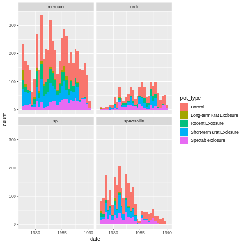
Let’s take a look at another code example. Our goal: to see which k-rat species appear in different plot types over the years.

R

# Example: identifying a more complex error

# Just k-rats
krats <- rodents %>% filter(genus == "Dipadomys") #filter the dataset to just include the kangaroo rat genus

# plot a histogram of how many observations are seen in each plot type over an x axis of years.
ggplot(krats, aes(year, fill = plot_type)) + 
  geom_histogram() +
  facet_wrap(~species)

ERROR

Error in `combine_vars()`:
! Faceting variables must have at least one value.

Uh-oh. Another error here, when we try to make a ggplot. But what is “combine_vars?” And then: “Faceting variables must have at least one value” What does that mean?

This is not an easily interpretable error message from ggplot, and our code looks like it should run. This time we put the data argument in the right place, we included aes(), and we didn’t misspell anything.

Considering this chunk of code, let’s take a step back. Is it possible that we’re looking at the wrong code? What if the error isn’t in the ggplot code itself? Let’s look at the krats dataset to make sure it looks normal.

R

krats

OUTPUT

# A tibble: 0 × 13
# ℹ 13 variables: record_id <dbl>, month <dbl>, day <dbl>, year <dbl>,
#   plot_id <dbl>, species_id <chr>, sex <chr>, hindfoot_length <dbl>,
#   weight <dbl>, genus <chr>, species <chr>, taxa <chr>, plot_type <chr>

It’s empty! Something must have gone wrong not with ggplot, but with the code we used to create the krats object.

Strategy 4: Using `print()` to show information

We can use a print statement to see which genera are included in the original rodents dataset.

R

print(rodents %>% count(genus))

OUTPUT

# A tibble: 12 × 2
   genus                n
   <chr>            <int>
 1 Ammospermophilus   136
 2 Baiomys              3
 3 Chaetodipus        382
 4 Dipodomys         9573
 5 Neotoma            904
 6 Onychomys         1656
 7 Perognathus        553
 8 Peromyscus        1271
 9 Reithrodontomys   1412
10 Rodent               4
11 Sigmodon           103
12 Spermophilus       151

This tells us two things. For one, we noticed that we have misspelled Dipodomys, which we can now fix.

Our print() call also tells us that we should expect a data frame with 9573 values after subsetting to the genus Dipodomys. This will be useful to check our work after fixing the misspelling.

R

# Example: identifying a more complex error

# Just k-rats
krats <- rodents %>% filter(genus == "Dipodomys") #filter the dataset to just include the kangaroo rat genus (fixed misspelling)

# check dimensions of krats
dim(krats) # 9573, as expected!

OUTPUT

[1] 9573   13

R

# plot a histogram of how many observations are seen in each plot type over an x axis of years.
ggplot(krats, aes(year, fill = plot_type)) + 
  geom_histogram() +
  facet_wrap(~species)

OUTPUT

`stat_bin()` using `bins = 30`. Pick better value with `binwidth`.

Our improved code here looks good. Checking the dimensions of our subsetted data frame using dim() function confirms we now have all the Dipodomys observations, and our plot is looking better.

Routinely printing out information about your dataset can be a good way to check that your intermediate results make sense.

Summary: Code first aid

Let’s update our list of code first aid strategies:

Callout

Code first aid strategies, detailed version

Identify the problem area

add print statements immediately upstream or downstream of problem areas
check the desired output from functions
see whether any intermediate output can be further isolated and examined separately

Act on parts of the error we can understand

interpreting error messages
changing input to a function
checking on the control flow of code (e.g. for loops, if/else)

Reading the R documentation for relevant functions

reading the documentation’s Description, Usage, Arguments, Details
testing out code from the Examples section

Quick online help with a search engine / generative LLM

Copying error messages for more interpretable explanations
Describing your error in the hopes of an already-solved solution
Seeing if an LLM generates equivalent error-free code solving the same goal

We can now understand these steps as a continuous cycle of zeroing in on the problem more and more precisely. Whenever one of the first aid steps helps us identify a part of the code that is failing, we can zoom in on that piece of code and restart the checklist.

If the first aid steps are enough to solve the problem, great! If not, we can stop trying once we get stuck or don’t understand anymore how the code is failing. At that point, we can isolate the specific code area and use it to create a reprex in order to get help from someone else. We’ll delve more into the process of creating a reprex in the next episode.

Challenge

Exercise 3: Isolating the problem

The following lines of code are not working correctly.

A. What type of error is this? B. Using the toolbox of code first aid strategies, can you isolate the problem area?

R

# Goal: run a chi square test to see whether kangaroo rat observations in the `control` plot type differ significantly between different plot_ids (hopefully not!)

control_plot_data <-  krats %>% filter(plot_type == "Control")

n_control_plots <- length(control_plot_data$plot_id)
exp_proportions <- rep(1/n_control_plots, n_control_plots)

plot_counts <- control_plot_data %>% group_by(plot_id) %>% summarize(n = n())

# Chisq test -- do count values vary significantly by plot id? 

chisq.test(plot_counts$n, p = exp_proportions)

ERROR

Error in chisq.test(plot_counts$n, p = exp_proportions): 'x' and 'p' must have the same number of elements

Show me the solution

An isolated version of the problem area might look like:

R

n_control_plots <- length(control_plot_data$plot_id)
exp_proportions <- rep(1/n_control_plots, n_control_plots)

# Chisq test -- do count values vary significantly by plot id? 

chisq.test(plot_counts$n, p = exp_proportions)

ERROR

Error in chisq.test(plot_counts$n, p = exp_proportions): 'x' and 'p' must have the same number of elements

If we decide to move the plot_counts line right after the first control_plot_data line, as plot_counts seems to be calculated correctly. Here, we can see there’s probably something wrong with the p argument: exp_proportions is very long, much longer than the number of control plots! Let’s solve the problem.

R

n_control_plots <- length(unique(control_plot_data$plot_id))
exp_proportions <- rep(1/n_control_plots, n_control_plots)

# Chisq test -- do count values vary significantly by plot id? 

chisq.test(plot_counts$n, p = exp_proportions)

OUTPUT


	Chi-squared test for given probabilities

data:  plot_counts$n
X-squared = 79.977, df = 7, p-value = 1.392e-14

We can see that some plots have significantly more or fewer counts than others! Observations of kangaroo rats are not random – rather, some plots seem to attract the kangaroo rats more than others.

When should I prepare my code for a reprex?

If you’ve isolated the problem area and tried using code first aid strategies, but the error persists, it may be time to get some help.

In a classroom setting, we may be used to raising our hand, pointing at our code, and saying “I’m not sure what’s wrong.” But outside of the classroom, helpers have limited time, bandwidth, and requisite knowledge to help. That’s why reproducing the problem with a reproducible example is an essential skill to getting unstuck: it allows you to ask for expert help with a problem that’s clearly identified, self-contained, and reproducible, and allows the expert to quickly see whether they’ve got the requisite skills to answer your question!

Back to our analysis: Mickey tries to get unstuck

Back in the lab, Mickey is happily coding along, exploring the data. Let’s follow their analysis and see how they use code first aid and prepare the code for a reprex.

Mickey is interested in understanding how kangaroo rat weights differ across species and sexes, so they create a quick visualization.

R

# Barplot of rodent species by sex
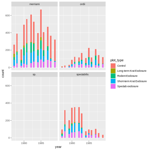
ggplot(surveys, aes(x = species, fill = sex)) +
  geom_bar()

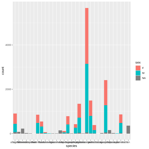
Whoa, this is really overwhelming! Mickey forgot that the dataset includes data for a lot of different species, not just kangaroo rats. Mickey is only interested in two kangaroo rat species: Dipodomys ordii (Ord’s kangaroo rat) and Dipodomys spectabilis (Banner-tailed kangaroo rat).

Mickey also notices that there are three categories for sex: F, M, and what looks like a blank field when there is no sex information available. For the purposes of comparing weights, Mickey wants to focus only rodents of known sex.

Mickey filters the data to include only the two focal species and only rodents whose sex is F or M.

R

# Filter to focal species and known sex
rodents_subset <- surveys %>%
  filter(species == c("ordii", "spectabilis"),
         sex == c("F", "M"))

Because these scientific names are long, Mickey also decides to add common names to the dataset. They start by creating a data frame with the common names, which they will then join to the rodents_subset dataset:

R

# Add common names
common_names <- data.frame(species = unique(rodents_subset$species), common_name = c("Ord's", "Banner-tailed"))
common_names

OUTPUT

      species   common_name
1 spectabilis         Ord's
2       ordii Banner-tailed

But looking at the common names dataset reveals a problem! The common names are not properly matched to the scientific names. For example, the genus Ordii should correspond to Ord’s kangaroo rat, but currently, it is matched with the Banner-tailed kangaroo rat instead.

Discussion

Challenge

Is this a syntax error or a semantic error? Explain why.
What “code first aid” steps might be appropriate here? Which ones are unlikely to be helpful?

Mickey re-orders the names and tries the code again. This time, it works! The common names are joined to the correct scientific names. Mickey joins the common names to rodents_subset.

R

# Try again, re-ordering the common names
common_names <- data.frame(species = sort(unique(rodents_subset$species)), common_name = c("Ord's", "Banner-Tailed"))
rodents_subset <- left_join(rodents_subset, common_names, by = "species")

Now, Mickey is ready to start learning about kangaroo rat weights. They start by running a quick linear regression to predict weight based on species and sex.

R

# Explore k-rat weights
weight_model <- lm(weight ~ species + sex, data = rodents_subset)
summary(weight_model)

OUTPUT


Call:
lm(formula = weight ~ species + sex, data = rodents_subset)

Residuals:
     Min       1Q   Median       3Q      Max
-109.531   -7.991    3.239   11.469   48.469

Coefficients: (1 not defined because of singularities)
                   Estimate Std. Error t value Pr(>|t|)
(Intercept)          47.991      1.136   42.23   <2e-16 ***
speciesspectabilis   73.540      1.420   51.79   <2e-16 ***
sexM                     NA         NA      NA       NA
---
Signif. codes:  0 '***' 0.001 '**' 0.01 '*' 0.05 '.' 0.1 ' ' 1

Residual standard error: 20.58 on 910 degrees of freedom
  (31 observations deleted due to missingness)
Multiple R-squared:  0.7466,	Adjusted R-squared:  0.7464
F-statistic:  2682 on 1 and 910 DF,  p-value: < 2.2e-16

The negative coefficient for common_nameOrd's tells Mickey that Ord’s kangaroo rats are significantly less heavy than Banner-tailed kangaroo rats.

But something is wrong with the coefficients for sex. Why are there NA values for sexM? Let’s directly visualize weight by species and sex to see.

R

# Weight by species and sex
rodents_subset %>%
  ggplot(aes(y = weight, x = species, fill = sex)) +
  geom_boxplot()

WARNING

Warning: Removed 31 rows containing non-finite outside the scale range
(`stat_boxplot()`).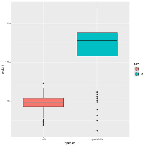

When Mickey visualizes the data, they see a problem in the graph, too. As the model showed, Ord’s kangaroo rats are significantly smaller than Banner-tailed kangaroo rats. But something is definitely wrong! Because the boxes are colored by sex, we can see that all of the Banner-tailed kangaroo rats are male and all of the Ord’s kangaroo rats are female. That can’t be right! What are the chances of catching all one sex for two different species?

To verify that the problem comes from the data, not from the plot code, Mickey creates a two-way frequency table, which confirms that there are no observations of female spectabilis or male ordii in rodents_subset. Something definitely seems wrong. Those rows should not be missing.

R

# Subsetted dataset
table(rodents_subset$sex, rodents_subset$species)

OUTPUT


    ordii spectabilis
  F   333           0
  M     0         610

To double check, Mickey looks at the original dataset.

R

# Original dataset
table(rodents$sex, rodents$species)

OUTPUT


    albigula eremicus flavus fulvescens fulviventer harrisi hispidus
  F      474      372    222         46           3       0       68
  M      368      468    302         16           2       0       42

    leucogaster maniculatus megalotis merriami ordii penicillatus  sp.
  F         373         160       637     2522   690          221    4
  M         397         248       680     3108   792          155    5

    spectabilis spilosoma taylori torridus
  F        1135         1       0      390
  M        1232         1       3      441

Not only were there originally males and females present from both ordii and spectabilis, but the original numbers were way, way higher! It looks like somewhere along the way, Mickey lost a lot of observations.

While we don’t have the time today, let’s assume Mickey worked their way through the code first aid steps, but weren’t able to solve the problem.

They decide to return to Remy’s road map to figure out what to do next.

Since code first aid was not enough to solve this problem, it looks like it’s time to ask for help using a reprex.

Key Points

The first step to getting unstuck is identifying a problem, isolating the problem area, and interpreting the problem
Often, using “code first aid” – acting on error messages, looking at data, inputs, etc., pulling up documentation, asking a search engine or LLM, can help us to quickly fix the error on our own.
If code first aid doesn’t work, we can ask for help and prepare a reproducible example (reprex) with a defined problem and isolated code
We’ll cover future steps to prepare a reproducible example (reprex) in future episodes.

Content from Minimal reproducible code

Last updated on 2025-08-26 | Edit this page

Overview

Questions

Why is it important to make a minimal code example?
Which part of my code is causing the problem?
Which parts of my code should I include in a minimal example?
How can I tell whether a code snippet is reproducible or not?
How can I make my code reproducible?

Objectives

Explain the value of a minimal code snippet.
Identify packages or other dependencies needed to run the code.
Simplify a script down to a minimal code example.
Evaluate whether a piece of code is reproducible as is or not. If not, identify what is missing.
Edit a piece of code to make it reproducible

When we left off in the previous episode, Mickey had discovered a problem with their code–many kangaroo rat observations were missing from a subset of the data after they filtered the dataset down to the kangaroo rat species of interest.

Mickey tried some code first aid steps but wasn’t able to solve the problem. They consulted Remy’s road map and saw that the next step is to make a reprex.

Making a reprex

Step 1: Minimize the code

Mickey has written a lot of code so far. The code is also a little messy–for example, after fixing the previous errors, they sometimes commented out the old code and kept it for future reference.

Let’s take a look at the script as it stands so far.

R

# Minimal reproducible example script
# Loading the tidyverse package
library(tidyverse)
# Uploading the dataset that is currently saved in the project's data folder
surveys <- read_csv("data/surveys_complete_77_89.csv")

# Take a look at the data
glimpse(surveys)

# or you can use
str(surveys)

table(surveys$taxa)

# Barplot of rodent species by sex
ggplot(rodents, aes(x = species, fill = sex)) +
  geom_bar()

# Filter to focal species and known sex
rodents_subset <- surveys %>%
  filter(species == c("ordii", "spectabilis"),
         sex == c("F", "M"))

# Add common names
# common_names <- data.frame(species = unique(rodents_subset$species), common_name = c("Ord's", "Banner-tailed"))
# common_names

# Try again, re-ordering the common names
common_names <- data.frame(species = sort(unique(rodents_subset$species)), common_name = c("Ord's", "Banner-Tailed"))
rodents_subset <- left_join(rodents_subset, common_names, by = "species")

# Explore k-rat weights
weight_model <- lm(weight ~ species + sex, data = rodents_subset)
summary(weight_model)

# Weight by species and sex
rodents_subset %>%
  ggplot(aes(y = weight, x = species, fill = sex)) +
  geom_boxplot()

# Subsetted dataset
table(rodents_subset$sex, rodents_subset$species)

# Original dataset
table(surveys$sex, surveys$species)

Discussion

Exercise 1: Reflection

As you look at this script and think through trying to debug it, how do you feel?
Mickey’s first instinct is to send the script to Remy and tell them about the error. Imagine that you are Remy, an advanced graduate student whose priority is finishing your dissertation. Your new labmate Mickey has just sent you this script, asking for help debugging it. How do you feel when you get Mickey’s email? What advice might you give Mickey?

When asking someone else for help, it is important to simplify your code as much as possible to make it easier for the helper to understand what is wrong. Simplifying code helps to reduce frustration and overwhelm when debugging an error in a complicated script. The more that we can make the process of helping easy and painless for the helper, the more likely it is that they will take the time to help.

Create a new script

Why do you think it’s a good idea to create a new script?

To make the task of simplifying the code less overwhelming, let’s create a separate script for our reprex. This will let us experiment with simplifying our code while keeping the original script intact.

Let’s create and save a new, blank R script and give it a name, such as “reprex-script.R”

Callout

Making an R script

There are several ways to make an R script:

File > New File > R Script
Click the white square with a green plus sign at the top left corner of your RStudio window
Use a keyboard shortcut: Cmd + Shift + N (on a Mac) or Ctrl + Shift + N (on Windows)

Let’s go ahead and copy over all of our code so we have an exact copy of the full analysis script. This way, we can make as many changes to it as we want and still keep the original code untouched.

Now, we will follow an iterative process to simplify our script.

A. Identify the symptom of the problem. What are you observing that shows you something is wrong?

B. Remove some code that is not central to demonstrating the problem.

C. Run the simplified code and make sure that the symptom is still present. Does your example still reproduce the problem?

A. Identify a symptom of the problem

Let’s figure out which line of code, when you run it, clearly shows that something is wrong. For a syntax error, this is straightforward: it’s the line of code that generates the error message. But our error here is a semantic error. The code runs, but it returns the wrong result. So let’s think instead about what line of code created a result that we could clearly see was incorrect.

This is a little tricky in our case, because we first noticed something was wrong when we looked at the output of the linear model. That model output could be a perfectly reasonable symptom to use!

R

summary(weight_model)

ERROR

Error: object 'weight_model' not found

But let’s not discount the work we’ve already done to diagnose this problem! Something looked strange about this model, so we made a plot. Something looked strange about the plot, so we double checked the dataset used to create both the model and the plot. By comparing that dataset with the original, un-subsetted data, we were able to determine that something was wrong.

To summarize, we have already determined:

The problem: There are many observations missing from rodents_subset that should not have been removed.

The symptom (lines that show that something is wrong): Comparison between the species and sex counts in the original and subsetted datasets.

In particular, this comparison shows us that there are no observations of female spectabilis or male ordii in rodents_subset, but there were plenty in the original dataset, and that in general, there were many fewer rows for both species in the subset than the original.

R

# Subsetted dataset
table(rodents_subset$sex, rodents_subset$species)

ERROR

Error: object 'rodents_subset' not found

R

# Original dataset
table(surveys$sex, surveys$species) # there are no observations of female spectabilis or male ordii in `rodents_subset`, even though there were in the original dataset.

OUTPUT


    albigula audubonii bilineata brunneicapillus chlorurus clarki eremicus
  F      474         0         0               0         0      0      372
  M      368         0         0               0         0      0      468

    flavus fulvescens fulviventer fuscus gramineus harrisi hispidus leucogaster
  F    222         46           3      0         0       0       68         373
  M    302         16           2      0         0       0       42         397

    leucophrys maniculatus megalotis melanocorys merriami ordii penicillatus
  F          0         160       637           0     2522   690          221
  M          0         248       680           0     3108   792          155

    scutalatus  sp. spectabilis spilosoma squamata taylori torridus viridis
  F          0    4        1135         1        0       0      390       0
  M          0    5        1232         1        0       3      441       0

These two lines of code, and the observation we made about them, will be our guide as we simplify the script further.

We can now start removing pieces of code that we believe are not central to our problem. After each removal, we can re-run the code and make sure that our symptom persists. If the symptom changes, we have either solved our problem (yay for rubber duck debugging!) or we removed a line of code that was actually essential to reproducing our problem.

B. Remove some code that is not central to demonstrating the problem.

Let’s start identifying pieces of code to remove. In general, we can remove code that does not create variables for later use (for example, exploratory plots, models, or descriptive functions such as head() or summary()). We can also get rid of code that adds complexity to the analysis that is not relevant to the problem at hand.

Let’s start by removing the broken code that we commented out earlier, back when we tried to join the common names and it didn’t work because they were in the wrong order.

Code to remove:

R

# Add common names
# common_names <- data.frame(species = unique(rodents_subset$species), common_name = c("Ord's", "Banner-tailed"))
# common_names

Actually, now that we think about it, those common names are not directly related to the problem at all! The “common_name” column might be useful later on, but for our reprex we can probably remove that part of the code without changing the outcome.

Code to remove:

R

# Try again, re-ordering the common names
common_names <- data.frame(species = sort(unique(rodents_subset$species)), common_name = c("Ord's", "Banner-Tailed"))
rodents_subset <- left_join(rodents_subset, common_names, by = "species")

After removing both of those pieces of code, our script is a little shorter:

R

# Minimal reproducible example script
# Loading the tidyverse package
library(tidyverse)
# Uploading the dataset that is currently saved in the project's data folder
surveys <- read_csv("data/surveys_complete_77_89.csv")

# Take a look at the data
glimpse(surveys)

# or you can use
str(surveys)

table(surveys$taxa)

# Barplot of rodent species by sex
ggplot(surveys, aes(x = species, fill = sex)) +
  geom_bar()

# Filter to focal species and known sex
rodents_subset <- surveys %>%
  filter(species == c("ordii", "spectabilis"),
         sex == c("F", "M"))

# Explore k-rat weights
weight_model <- lm(weight ~ species + sex, data = rodents_subset)
summary(weight_model)

# Weight by species and sex
rodents_subset %>%
  ggplot(aes(y = weight, x = species, fill = sex)) +
  geom_boxplot()

# Subsetted dataset
table(rodents_subset$sex, rodents_subset$species)

# Original dataset
table(surveys$sex, surveys$species)  # there are no observations of female spectabilis or male ordii in `rodents_subset`, even though there were in the original dataset.

C. Run the simplified code and make sure that the symptom is still present. Does your example still reproduce the problem?

Now it’s time to re-run the script to make sure we haven’t removed anything essential. Remember to pay attention to the symptom of the problem at the end and make sure that the essential observation hasn’t changed. Sure enough, those observations are still missing. We have succeeded in simplifying our code while still demonstrating the problem!

Great progress, but this script is still pretty long and complicated. Can we remove more things?

Challenge

Exercise 2: Minimizing code

Minimizing code is an iterative process. Repeat steps B and C above several more times. Which other lines of code can you remove to make this script more minimal? After removing each part, be sure to re-run the code to make sure that it still reproduces the error.

Show me the solution

The barplot of species and sex (ggplot) can be removed because it generates a plot but does not create any variables that are used later.
Similarly, our end visualization of weight by species and sex (boxplot) can be removed.
The weight model and the summary can be removed
Any other informational functions that could have been run in the console, such as table() or print(), head(), or str() can be removed.
The essential parts to keep are the lines that access the dataset in the first place, subset it down to rodents_subset, and then diagnose the problem (the table() calls at the end).

After repeating steps B and C over and over again, we arrive at a much more minimal script.

R

# Loading the tidyverse package
library(tidyverse)

surveys <- read_csv("data/surveys_complete_77_89.csv")

# Filter to focal species and known sex
rodents_subset <- surveys %>%
  filter(species == c("ordii", "spectabilis"),
         sex == c("F", "M"))

# Subsetted dataset
table(rodents_subset$sex, rodents_subset$species)

# Original dataset
table(surveys$sex, surveys$species) # there are no observations of female spectabilis or male ordii in `rodents_subset`, even though there were in the original dataset.

Mickey is really getting the hang of this! They scrutinize the example to see if there’s anything else that can be cut. They realize that the code still runs perfectly fine if they remove library(tidyverse)–since they already loaded the {tidyverse} package, there should be no need to load it again!

Mickey realizes that they might be able to narrow the example down eeeeeeven more. They try removing the species filter and only filtering by sex. Now the minimal example looks like this:

R

surveys <- read_csv("data/surveys_complete_77_89.csv")

# Filter to known sex
rodents_subset <- surveys %>%
  filter(sex == c("F", "M"))

# Subsetted dataset
table(rodents_subset$sex, rodents_subset$species)

# Original dataset
table(surveys$sex, surveys$species) # still missing a lot of rows!

Something is different–we no longer have zero rows for two of the species/sex combos. But this example still demonstrates our problem. Remember, we previously stated the problem as “There are many observations missing from rodents_subset that should not have been removed.” And sure enough, if we look closely here, we can see that our species/sex counts have changed from 690 F ordii/792 M ordii and 1135 F spectabilis/1232 M spectabilis to 333/393 and 568/610, respectively. The problem persists! We are still mysteriously missing rows.

Callout

If you had chosen to remove the sex filter instead of removing the species filter, the same point would be made. The numbers would be different, but we would still see fewer rows in the subsetted data frame. Either one works!

Callout

If you hadn’t noticed that you could simplify this example even further, that would still be okay! Minimizing code is an art, not an exact science. The more minimal you can make your code, the better, but a helper will still have a much easier time working on your problem if you’ve removed some extraneous steps, even if you haven’t narrowed it down 100%. Don’t let the perfect be the enemy of the good!

Okay, so our minimal snippet looks like this:

R

surveys <- read_csv("data/surveys_complete_77_89.csv")

# Filter to known sex
rodents_subset <- surveys %>%
  filter(sex == c("F", "M"))

# Subsetted dataset
table(rodents_subset$sex, rodents_subset$species)

# Original dataset
table(surveys$sex, surveys$species) # still missing a lot of rows!

This is great progress! Remy will find this minimal code snippet much more approachable than the long script that Mickey started with.

Discussion

Exercise 3: Have we made a reprex?

Mickey is really proud of their efforts to minimize the code! They email the minimal code snippet to Remy to ask for help. Remy notices immediately that this code is much easier to read and understand. They open up the script and try to run it in R.

What do you think will happen when Remy tries to run the code from this reprex script?
What should Mickey do next to improve the minimal reproducible example?

We haven’t yet included enough code to allow a helper, such as Remy, to run the code on their own computer. If Remy tries to run the reprex script in its current state, they will encounter errors because they don’t have access to the same R environment that Mickey does.

That’s why it’s so important to include dependencies in your reprex.

Include dependencies

A dependency is a piece of code that other pieces of code depend on in order to function properly.

R code consists primarily of functions and variables. In order to make our minimal examples truly reproducible, we have to give our helpers access to all the functions and all the variables that are necessary to run our code.

First, let’s talk about functions. Functions in R typically come from packages. You can access them by loading the package into your environment.

To make sure that your helper has access to the packages necessary to run your reprex, you will need to include calls to library() for whichever packages are used in the code. For example, if your code uses the function lmer from the lme4 package, you would have to include library(lme4) at the top of your reprex script to make sure your helper has the lme4 package loaded and can run your code.

Callout

Default packages

Some packages, such as {base} and {stats}, are loaded in R by default, so you might not have realized that a lot of commonly-used functions, such as dim, colSums, mean, and length actually come from those packages!

You can see a complete list of the functions that come from the {base} and {stats} packages by running library(help = "base") or library(help = "stats") in your console.

But, you actually don’t need to worry too much about this because your helpers’ RStudio versions will also have {base} and {stats} preinstalled!

Let’s do this for our own reprex. We can start by identifying all the functions used, and then we can figure out where each function comes from to make sure that we tell our helper to load the right packages.

Discussion

Exercise 4: Which packages should we load?

The functions used in our minimal example are read_csv(), filter(), c(), and table().

Identify the package that each of the functions comes from and modify the minimal example so that it explicitly loads those packages. :::solution library(dplyr) library(readr)

filter() comes from dplyr, and read_csv()comes from{readr}.c()andtable()come from{base}`, which is loaded by default, so we don’t need to include a library() call for this.

Bonus if you notice that we also use the %>% operator, which comes from dplyr too, so we definitely need to make sure that dplyr is loaded!

Extra challenge: did we use any other operators? Where do they come from?

:::

We can update our minimal code to include those library() calls.

R

library(readr)
library(dplyr)

surveys <- read_csv("data/surveys_complete_77_89.csv")

# Filter to known sex
rodents_subset <- surveys %>%
  filter(sex == c("F", "M"))

# Subsetted dataset
table(rodents_subset$sex, rodents_subset$species)

# Original dataset
table(surveys$sex, surveys$species) # still missing a lot of rows!

Callout

Installing vs. loading packages

We included calls to library() to load the packages we need. But what if our helper doesn’t have all of these packages installed? Won’t the code not be reproducible?

Packages need to be installed one time before they can be loaded with library(). Typically, we don’t include install.packages() in our code for each of the packages that we include in the library() calls, because install.packages() doesn’t need to be repeated every time the script is run. We can assume that our helper will see library(specialpackage) and know that they need to go install “specialpackage” on their own.

Technically, this does make that part of the code not reproducible! But it’s also more “polite” than explicitly including install.packages(). Our helper might have their own way of managing package versions, and forcing them to install a package when they run our reprex risks messing up their workflow. It is a common convention to stick with library() and let the helper figure it out from there.

Discussion

Exercise 5: Which packages are essential?

In each of the following code snippets, identify the necessary packages (or other code) to make the example reproducible.

weight_model <- lm(weight ~ common_name + sex, data = rodents_subset)
tab_mod(weight_model)

mod <- lmer(weight ~ hindfoot_length + (1|plot_type), data = rodents)
summary(mod)

rodents_processed <- process_rodents_data(rodents)
glimpse(rodents_processed)

This exercise should take about 10 minutes. :::solution a. lm is part of base R, so there’s no package needed for that. tab_mod comes from the package sjPlot. You could add libary(sjPlot) to this code to make it reproducible. b. lmer is a linear mixed modeling function that comes from the package lme4. summary is from base R. You could add library(lme4) to this code to make it reproducible. c. process_rodents_data is not from any package that we know of, so it was probably an originally-created function. In order to make this example reproducible, you would have to include the definition of process_rodents_data. glimpse is probably from dplyr, but it’s worth noting that there is also a glimpse function in the pillar package, so this might be ambiguous. This is another reason it’s important to specify your packages–if you leave your helper guessing, they might load the wrong package and misunderstand your error!

:::::::::::::::::::::::::::::::::::::::::::

Including library() calls will definitely help Remy run the code. But this code still won’t work as written because Remy does not have access to the same objects that Mickey used in the code. Along with functions, objects are the second type of dependency we need to watch out for when writing reprexes.

The code as written relies on rodents_subset, which Remy will not have access to if they try to run the code. That means that we’ve succeeded in making our example minimal, but it is not reproducible: it does not allow someone else to reproduce the problem!

In the next episode, we will learn how to handle perhaps the most thorny part of creating reprexes: dealing with datasets.

Discussion

Exercise 6: Reflection

Let’s take a moment to reflect on this process.

What’s one thing you learned in this episode? An insight; a new skill; a process?
What is one thing you’re still confused about? What questions do you have?

This exercise should take about 5 minutes.

Key Points

Making a reprex is the next step after trying code first aid.
In order to make a good reprex, it is important to simplify your code
Simplify code by removing parts not directly related to the question
Give helpers access to the functions used in your code by loading all necessary packages

Content from Minimal reproducible data

Last updated on 2025-08-26 | Edit this page

Overview

Questions

What is a minimal reproducible dataset, and why do I need it?
How do I create a minimal reproducible dataset?
Can I just use my own data?

Objectives

Describe a minimal reproducible dataset
Appreciate the different approaches and viewpoints on providing example data
Identify the relevant aspects of your data
Create a suitable reprex dataset from scratch
Share your own dataset in a way that is minimal, accessible, and reproducible
Subset a built-in dataset to use in your reprex

4.1 What is a minimal reproducible dataset and why do I need it?

Now that Mickey has narrowed down their problem area and stripped down their code to make it minimal, they need to ensure it is reproducible; this means it needs to be accessible and executable such that anyone else can simoly copy-paste the code into their system and replicate their issue. Importantly, a code snippet will usually require data objects in order to run! Therefore, every reprex requires a minimal reproducible dataset to use with the code.

Furthermore, as we have seen previously, sometimes the source of the problem isn’t actually the code, but rather the data! Providing an appropriate example, or mock dataset allows a helper to better investigate and manipulate that data to fix the problem.

Callout

Remember: your helper may not have access to your computer and files!

You might be used to always uploading data from separate files, but helpers can’t access those files. Even if you sent someone a file, they would need to put it in the right directory, make sure to load it in exactly the same way, make sure their computer can open it, etc. Since the goal is to make everyone’s lives as easy as possible, we need to think about our data in a different way–as a mock object created in the script itself.

As with the code, a reprex dataset should also be minimal–free of unnecessary information. By removing extraneous information and only keeping what is required to replicate the issue, we can ensure our helper will be able to easily see how the data is structured and where the problem arises. While it may sometimes feel like unnecessary effort, the process of creating a minimal dataset will not only help others help you, but also allow you to better understand your data and often discover the source of the problem without the need for external help.

In summary, just like with the code, a minimal reproducible dataset must be:

minimal: it only contains information required to run your minimal code. You can also think of this as being relevant to the problem (keep only what is necessary).
reproducible: it must be accessible to someone without your computer, and it must consistently replicate your problem. This means it also needs to be complete, meaning there are no dependencies that have been omitted (e.g., packages).

Callout

Pro-tip

An example of what minimal reproducible examples look like can also be found in the ?help section, in R Studio. Just scroll all the way down to where there are examples listed. These will usually be minimal and reproducible, since they are intended to be directly copy-pasted and run by anyone.

For example, let’s look at the function mean:

R

?mean

We see examples that can be run directly on the console, with no additional code.

R

x <- c(0:10, 50)
xm <- mean(x)
c(xm, mean(x, trim = 0.10))

OUTPUT

[1] 8.75 5.50

In this case, x is the mock dataset consisting of just 1 variable. Notice how it was created as part of the example. This will be your goal with your reprex.

Challenge

Exercise 1: Test your knowledge! (3 mins)

The datasets listed below are not well suited for use in a reprex. Can you explain why? Copy each one onto your own R script to check whether they are reproducible. What did you find?

sample_data <- read_csv(“/Users/kaija/Desktop/RProjects/ResearchProject/data/sample_dataset.csv”)
sample_data <- data.frame(species = species_vector, weight = c(10, 25, 14, 26, 30, 17))

Show me the solution

Not reproducible because it is a screenshot.
Not reproducible because it is a path to a file that only exists on someone else’s computer and therefore you do not have access to it using that path.
Not reproducible because we are not given the source for species_vector.

Challenge

Extra Practice (optional)

Let’s say we want to know the average weight of all the species in our rodents dataset. We try to use the following code…

R

mean(rodents$weight)

OUTPUT

[1] NA

…but it returns NA! We don’t know why that is happening and we want to ask for help.

Which of the following represents a minimal reproducible dataset for this code? Can you describe why the other ones are not?

sample_data <- data.frame(month = rep(7:9, each = 2), hindfoot_length = c(10, 25, 14, 26, 30, 17))
sample_data <- data.frame(weight = rnorm(10))
sample_data <- data.frame(weight = c(100, NA, 30, 60, 40, NA))
sample_data <- sample(rodents$weight, 10)
sample_data <- rodents_modified[1:20,]

Show me the solution

The correct answer is C!

does not include the variable of interest (weight).
does not produce the same problem (NA result with a warning message)–the code runs just fine.
minimal and reproducible.
is not reproducible. Sample randomly samples 10 items; sometimes it may include NAs, sometime it may not (not guaranteed to reproduce the error). It can be used if a seed is set (see next section for more info).
uses a dataset that isn’t accessible without previous data wrangling code–the object rodents_modified doesn’t exist.

4.2 Can I just use my own data?

While Mickey is grateful to Remy for providing them with a roadmap to follow when they need help, they still feel it would be much easier and faster to just send Remy their whole dataset rather than creating a different one. If they give Remy access to everything, can’t he still help?

Challenge

Exercise 2: Reflect (3 mins)

When Mickey feels like sharing their own data would be easier, for whom do you think they are referring? Who would find it easier, Mickey or Remy?
Can you think of any reasons why sharing the original data may not be possible or recommended?

Show me the solution

Mickey is thinking that it would be easier for themselves, not necessarily for Remy.

Remember: one of the goals of creating a reprex is to help the helpers. They don’t have to help, they are volunteering their time. As such, they deserve to be treated with kindness and respect. If you find yourself getting frustrated at how much time and effort creating a reprex might be taking, remember that (1) trusting the process may reveal the solution along the way; and (2) being kind, clear, and helpful will reward you with a quicker, more accurate solution.
There are several reasons why sharing the original data may not be possible or recommended. The original dataset may be:

too large - the Portal dataset is ~35,000 rows with 13 columns and contains data for decades. That’s a lot!
private - the dataset might not be published yet, it may not be yours to share, or maybe it includes protected information such as personal medical information or the location of endangered species.
hard to send - on most online forums, you can’t attach supplemental files (more on this later). Even if you are just sending data to a colleague, file paths can get complicated, the data might be too large to attach, etc.
complicated - it would be hard to locate the relevant information. One example to steer away from are needing a ‘data dictionary’ to understand all the meanings of the columns (e.g. what is “plot type” in ratdat?) We don’t our helper to waste valuable time to figure out what everything means.
highly derived/modified from the original file. You may have already done a bunch of preliminary data wrangling you don’t want to include when you send the example, so you would need to provide the intermediate dataset directly to your helper.

Mickey is not entirely wrong. While there are instances when it is not possible or advisable to share original data, there are also many ways around such challenges and some instances may indeed benefit from keeping the original data. However, it is still important to provide helpers with data that is minimal and reproducible. Therefore, while Mickey does not have to create a brand new example dataset, they should at least work to make their original data minimal and accessible (see the above reflection exercise), and this may not end up being easier or faster than creating a mock dataset from scratch.

In summary, there are multiple ways to provide a minimal, reproducible dataset for a reprex, including using a simplified version of the original dataset. In the following section we will highlight 3 common approaches.

4.3 Three different approaches

In general, there are 3 common ways to provide minimal reproducible data for a reprex.

Add a few lines of code to create a mock dataset with the same key characteristics as the original data.
Subset the original data to be minimal and reproducible.
Subset a dataset that is already provided by R (e.g., cars, npk, penguins, etc.). For a complete list, use library(help = "datasets").

Callout

Pros and Cons

The developers of this lesson believe everyone is entitled to use any option they prefer, therefore the rest of this episode will expand on each of the 3 approaches listed above. However, within the data science community, opinions differ on which method is best recommended. Below is a summary table of advantages and disadvantages of each approach based on many conversations with several data science groups.

	Advantages	Disadvantages
Data from Scratch	Often the most concise Easiest for helpers Helps problem-solve along the way (e.g., identify what data aspects are generating the problem) More universally applicable: Easy to share, collaborate, teach, and understand Avoids privacy/security concerns Lets you clearly illustrate the sought outcome Uses important-to-learn skills Easier with practice	Can be intimidating Requires good understanding of your data Harder to generate if the error is idiosyncratic or dependent on having a large dataset Time-consuming if unpracticed Iterative (you may need to trial and error a few times to replicate the problem) More likely to require analogies, less interpretable/concrete, more likely to require greater context Risks generating XY problems–make sure you are asking the right question/replicating the right problem
R-built Data	Simple and easy to share–no need to provide additional data Familiar–helpers already know the data structure Potentially faster than starting from scratch (i.e. faster than generating rows/columns de novo). No privacy/security concerns Can easily be manipulated or simplified Generalizes the problem	May require a good mental model of the problem Harder if the error is idiosyncratic Greatest risk of generating XY problems–make sure you are asking the right question/replicating the right problem Iterative (you may need to trial and error a few times to replicate the problem) Need to re-think the question so it matches a different dataset and context–mental gymnastics Still need to choose which dataset and variables are more appropriate
Your Data	Can require the least mental effort Problem is easy to replicate even if you don’t understand it at all Accurately represents the actual problem; avoids XY problems. Richer context may intrigue/motivate helpers Can be quicker if dataset is small May be required for idiosyncratic problems that are based on aspects of the data itself that you don’t know about (e.g. when the data itself, rather than the code per se, is central to the problem) Captures data structures that are difficult or time-consuming to replicate if you are a novice	Less growth-minded if chosen as an “easy way out”–skips the learning process and any insights you could have gained. Easy to do poorly and think that you’re doing it well; perceived “easiness” leads to overcomplication/confusion Leaves all the work to the helpers if you don’t also work to minimize it–less motivation for harder work Could obfuscate the problem if not minimized–less likely to find a quick answer More difficult to share–may be large/messy Security/privacy/sanitizeation problems

4.4 Creating a mock dataset from scratch

While starting from scratch can be daunting at first, it becomes easier and faster with practice. Once you are familiar with the basic building blocks, it is a very straight-forward method of creating a minimal reproducible dataset. This is also the preferred method for other activities that require a reprex (e.g., teaching, collaborating, developing, etc.), and it often provides valuable problem-solving insights. So let’s breakdown this process to be more digestible!

Mickey is still new at this and has 2 pressing questions:

How do I create a dataset from scratch?
How do I know which key aspects of my data to recreate?

Let’s start with the first.

There are many ways one can create a dataset in R (these should be familiar if you took the Carpentries lesson Data Analysis and Visualization in R for Ecologists).

You can start by creating vectors using c()

R

vector <- c(1,2,3,4) 
vector

OUTPUT

[1] 1 2 3 4

You can also add some randomness by sampling from a vector using sample().

For example you can sample numbers 1 through 10 in a random order

R

x <- sample(1:10)
x

OUTPUT

 [1]  7  8  4  6  1 10  3  5  2  9

Or you can randomly sample from a normal distribution

R

x <- rnorm(10)
x

OUTPUT

 [1]  0.2513454  0.5913126 -1.3471443  0.8039914  0.1522019  0.5335401
 [7] -0.6697545  0.6394825 -0.3165660 -0.8280896

You can also use letters to create factors.

R

x <- sample(letters[1:4], 20, replace=T)
x

OUTPUT

 [1] "c" "d" "a" "c" "d" "c" "a" "a" "a" "b" "b" "b" "d" "b" "b" "d" "a" "a" "b"
[20] "b"

Remember that a data frame is just a collection of vectors. You can create a data frame using data.frame (or tibble in the dplyr package), and then define a vector for each variable.

R

data <- data.frame (x = sample(letters[1:3], 20, replace=T), 
                    y = rnorm(1:20))
head(data)

OUTPUT

  x          y
1 a -0.3781020
2 c -0.2510934
3 c -0.6544835
4 c  1.9972867
5 c -0.2187458
6 b -1.7033189

However, when sampling at random you must remember to set.seed() before sending it to someone to make sure you both get the same numbers!

Callout

For more handy functions for creating data frames and variables, see the [cheatsheet]. Some questions may require specific formats. For these, you can use any of the provided as.someType functions: as.factor, as.integer, as.numeric, as.character, as.Date, as.xts.

Discussion

Exercise 3: You try! (5 mins)

Create a data frame with:

A. One categorical variable with 2 levels and one continuous variable.

B. One continuous variable that is normally distributed.

C. Name, sex, age, and treatment type.

4.5 Identifying the relevant aspects of your data

No matter which approach you choose to take for providing a dataset, they key is always to identify which elements of the original data are necessary, or relevant, to replicate the problem. To do so, here are a few guiding questions:

Which variables are necessary to replicate the problem?
What data type (discrete or continuous) is each variable?
How many levels and/or observations are necessary?
Do the values need to be distributed in a specific way?
Are there any NAs that could be relevant?

Let’s check back with Mickey and the minimal code they settled on:

R

# Mickey's minimal code [ UPDATE AS NEEDED ]

library(dplyr)
library(ggplot2)

rodents<-read.csv('data/surveys_complete_77_89.csv')

rodents_subset <- rodents %>%
  filter(species == c("ordii", "spectabilis"),
         sex == c("F", "M"))

table(rodents_subset$sex, rodents_subset$species)

OUTPUT


    ordii spectabilis
  F   333           0
  M     0         610

R

table(rodents$sex, rodents$species)

OUTPUT


    albigula audubonii bilineata brunneicapillus chlorurus clarki eremicus
          62        69       223              23        11      1       14
  F      474         0         0               0         0      0      372
  M      368         0         0               0         0      0      468

    flavus fulvescens fulviventer fuscus gramineus harrisi hispidus leucogaster
        15          0           0      2         3     136        2          16
  F    222         46           3      0         0       0       68         373
  M    302         16           2      0         0       0       42         397

    leucophrys maniculatus megalotis melanocorys merriami ordii penicillatus
             2           9        33          13       45     3            6
  F          0         160       637           0     2522   690          221
  M          0         248       680           0     3108   792          155

    scutalatus  sp. spectabilis spilosoma squamata taylori torridus viridis
             1   18          42       149       16       0       28       1
  F          0    4        1135         1        0       0      390       0
  M          0    5        1232         1        0       3      441       0

To make sure Remy can work on this anywhere, Mickey needs to ensure he has the required dataset to run the code.

Challenge

Exercise 4: Quick, think! (2 mins)

Based on the current minimal code, which dataset does Mickey need to recreate? Hint: they currently have two datasets, rodents and rodents_subset.

Show me the solution

Mickey needs to provide a mock dataset to replace the original rodents dataset.

Let’s take a closer look at the dataset we need to substitute and then answer the questions outlined earlier.

R

head(rodents)

OUTPUT

  record_id month day year plot_id species_id sex hindfoot_length weight
1         1     7  16 1977       2         NL   M              32     NA
2         2     7  16 1977       3         NL   M              33     NA
3         3     7  16 1977       2         DM   F              37     NA
4         4     7  16 1977       7         DM   M              36     NA
5         5     7  16 1977       3         DM   M              35     NA
6         6     7  16 1977       1         PF   M              14     NA
        genus  species   taxa                plot_type
1     Neotoma albigula Rodent                  Control
2     Neotoma albigula Rodent Long-term Krat Exclosure
3   Dipodomys merriami Rodent                  Control
4   Dipodomys merriami Rodent         Rodent Exclosure
5   Dipodomys merriami Rodent Long-term Krat Exclosure
6 Perognathus   flavus Rodent        Spectab exclosure

Discussion

Exercise 5: Your turn! (5 mins)

Try to answer the following questions on your own to determine what we need to include in our minimal reproducible dataset:

Which variables does Mickey need to replicate their problem?
What data type (discrete or continuous) is each variable?
How many levels and/or observations are necessary?
Do the values need to be distributed in a specific way?
Are there any NAs that could be relevant?

Let’s go over the answers together and help Mickey build a dataset as we go along!

How many variables does Mickey need to reproduce their problem?

They need species, sex, and maybe a third identifier like record_id. This means they potentially need 3 vectors (remember, each column in a dataframe is essentially a vector, and in “tidy data” should correspond with a variable; each row is then an observation).

R

# create 3 variables: species, sex, and maybe record_id

# a vector for species:

# a vector for sex:

# a vector for record_id:

What data type (discrete or continuous) is each variable?

Species and sex are both discrete (categorical) variables, while record ID would be more continuous.

R

# create 3 variables: species, sex, and maybe record_id

# a vector for species: categorical 

# a vector for sex: categorical

# a vector for record_id: continuous

How many levels and/or observations are necessary?

Since Mickey is filtering their dataset down to 2 categories for both species and sex, that means they need at least 3 levels in each to start with. In terms of number of observations there don’t seem to be specific restrictions other than they probably want at least 1 observation per original category, so 2*3=6, or they can just pick a generally nice number like 10. This is where creating a reprex dataset becomes a bit more of an art than a science; it is common to use trial and error until the problem is replicated accurately.

R

# create 3 variables: species, sex, and maybe record_id

# a vector for species: categorical with 3 levels 

# a vector for sex: categorical with 3 levels 

# a vector for record_id: continuous, ~10

Do the values need to be distributed in a specific way?

This question probably isn’t going to be relevant most of the time, but certainly worth considering. If Mickey needed a longer dataset of measurements they may have wanted to make sure it was normally distributed. If they needed a longer dataset of counts they may have wanted to make sure it was Poisson distributed. Or maybe they had binary data. But in this case, Mickey has a fairly short dataset and the code doesn’t include anything that should vary depending on the distribution, so it probably doesn’t matter. Again, this process can be one of trial and error. They can always come back to this question if they are unable to replicate their problem (hint: in which case the distribution may be related to the problem they are having!).

Are there any NAs that could be relevant?

Mickey’s data does have NAs for the sex variable. It might not matter or it could be important, so let’s have them put in NAs in the mock dataset just in case.

R

# create 3 variables: species, sex, and maybe record_id

# a vector for species: categorical with 3 levels
species <- sample(letters, 3, replace=F) 
          # or name 3 categories like we do with sex below
species

OUTPUT

[1] "p" "a" "g"

R

# a vector for sex: categorical with 3 levels, one of which is NA 
sex <- c('M','F',NA)
sex

OUTPUT

[1] "M" "F" NA

R

# a vector for record_id: continuous, ~10 
record_id <- 1:10 
record_id

OUTPUT

 [1]  1  2  3  4  5  6  7  8  9 10

R

# Now let's go "sampling" and put our "obervations" in a dataframe
sample_data <- data.frame(
  # record_id stays the same, since these are our 10 "observations"
  record_id = record_id,
  # randomly select 10 observations from our list of species
  species = sample(species, 10, replace=T),
  # randomly select 10 observations from our list of sexes
  sex = sample(sex, 10, replace=T)
)

# Look at our new dataset
sample_data

OUTPUT

   record_id species  sex
1          1       p    F
2          2       a    M
3          3       p    F
4          4       a    F
5          5       a    M
6          6       p    M
7          7       g    F
8          8       p    F
9          9       p <NA>
10        10       a    M

And just like that we helped Mickey create a mock dataset from scratch! Notice that they could also have compiled the same type of dataset in a single line by creating each vector within data.frame()

R

sample2_data <- data.frame(
  record_id = 1:10,
  species = sample(letters[1:3], 10, replace=T),
  sex = sample(c('M','F', NA), 10, replace=T)
)

sample2_data

OUTPUT

   record_id species  sex
1          1       b    M
2          2       a    F
3          3       a    M
4          4       b    F
5          5       c    F
6          6       a    F
7          7       a    M
8          8       c    M
9          9       a    M
10        10       c <NA>

Important: Notice that the outputs of the two datasets are not the same. If you want the outputs to be EXACTLY the same each time, but you are using sample() which is an inherently random process, you must first use set.seed() and share that with your helper too.

R

set.seed(1) # set seed before recreating the sample
sample_data <- data.frame(
  record_id = 1:10,
  species = sample(letters[1:3], 10, replace=T),
  sex = sample(c('M','F', NA), 10, replace=T)
)
sample_data

OUTPUT

   record_id species  sex
1          1       a <NA>
2          2       c    M
3          3       a    M
4          4       b    M
5          5       a    F
6          6       c    F
7          7       c    F
8          8       b    F
9          9       b <NA>
10        10       c    M

Callout

Adding a set.seed() at the start of your reprex will ensure anyone else who runs the same code in the same order will always get the same results. However, if using it more generally, you may want to read more about it. For example, in the example below we set a seed of 2 and then run sample(10) twice. You will notice that the output of each sample run is not the same. However, if you run the whole code again, you will see that each of the outputs actually do stay the same.

R

set.seed(2)
sample(10)

OUTPUT

 [1]  5  6  9  1 10  7  4  8  3  2

R

sample(10)

OUTPUT

 [1]  1  3  6  2  9 10  7  5  4  8

Great! Now we need to check whether the mock dataset works with the minimal code Mickey created earlier. Does it run? Does it replicate the problem they were having?

R

# Minimal code [or whatever we end up with] 
sample_subset <- sample_data %>% # replace rodents with our sample dataset
  filter(species == c("a", "b"), # replace species with those from our sample dataset
         sex == c("F", "M")) # this can stay the same because we recreated it the same

table(sample_subset$sex, sample_subset$species)

OUTPUT


    a b
  F 1 0
  M 0 1

It works! The sample size has unexpectedly been reduced to just 2 observations, when we would have expected a sample of 8, based on the sample_data output above. Wherever the issue may lie, we were able to successfully replicate it in this minimal reproducible example.

4.6 Using the original data set

Even if you master the art of creating mock datasets, there may be occasions in which your data or problem is too complex and you can’t seem to replicate the issue. Or maybe you still think using your original data would just be easier.

In cases when you want to make your own data minimal and reproducible, you will want to take a similar approach to what we did in Episode 3 when making the code minimal. Keep what is essential, get rid of the rest. In other words, we will want to subset our data into a smaller, more digestible chunk.

The question still arises: how do I know what is essential?

Use the same guiding questions that we used earlier!

Which variables are necessary to replicate the problem?
What data type (discrete or continuous) is each variable? (perhaps less necessary, since you are keeping the original variables)
How many levels and/or observations are necessary? (we don’t want to get rid of more than we need)
Do the values need to be distributed in a specific way? (worth keeping in mind in terms of how we are removing observations)
Are there any NAs that could be relevant?

Based on our previous answers we end up with:

We need species, sex, and maybe record_id
Species and sex are categorical, record_id is a continuous count of our observations.
As we said earlier, we want 3 each for species and sex, which happens to already be the case. And we could reduce our record_id size to ~10.
Not really, but we want to make sure that when we reduce the number of observations we still have observations in each of the 3 levels in species and sex.
NA’s are present in the sex variable, so let’s make sure we keep at least one.

Now that we have a clearer goal, let’s subset the data.

Useful functions for subsetting a dataset include subset(), head(), tail(), and indexing with [] (e.g., iris[1:4,]). Alternatively, you can use tidyverse functions like select(), and filter() from the tidyverse. You can also use the same sample() functions we covered earlier.

Note: you should already have an understanding of how to subset or wrangle data using the tidyverse from the Data Analysis and Visualization in R for Ecologists. If not, go check it out!

R

# Mickey's minimal code [ UPDATE AS NEEDED ]

library(dplyr)
library(ggplot2)

rodents<-read.csv('data/surveys_complete_77_89.csv')

rodents_subset <- rodents %>%
  filter(species == c("ordii", "spectabilis"),
         sex == c("F", "M"))

table(rodents_subset$sex, rodents_subset$species)

OUTPUT


    ordii spectabilis
  F   333           0
  M     0         610

R

table(rodents$sex, rodents$species)

OUTPUT


    albigula audubonii bilineata brunneicapillus chlorurus clarki eremicus
          62        69       223              23        11      1       14
  F      474         0         0               0         0      0      372
  M      368         0         0               0         0      0      468

    flavus fulvescens fulviventer fuscus gramineus harrisi hispidus leucogaster
        15          0           0      2         3     136        2          16
  F    222         46           3      0         0       0       68         373
  M    302         16           2      0         0       0       42         397

    leucophrys maniculatus megalotis melanocorys merriami ordii penicillatus
             2           9        33          13       45     3            6
  F          0         160       637           0     2522   690          221
  M          0         248       680           0     3108   792          155

    scutalatus  sp. spectabilis spilosoma squamata taylori torridus viridis
             1   18          42       149       16       0       28       1
  F          0    4        1135         1        0       0      390       0
  M          0    5        1232         1        0       3      441       0

Given that the code that is going wrong is that which creates rodents_subset, we need to create a minimal reproducible version of rodents! We can then insert our new_rodents dataset in place of the original rodents one.

Step 1: select the variables of interest

R

# subset rodent into new_rodent to make it minimal
# Note: there are many ways you could do this!
new_rodents <- rodents %>% 
  # 1. select the variables of interest
  select(record_id, species, sex)
  # PAUSE. Does this work so far?
new_rodents

OUTPUT

   record_id      species sex
1          1     albigula   M
2          2     albigula   M
3          3     merriami   F
4          4     merriami   M
5          5     merriami   M
6          6       flavus   M
7          7     eremicus   F
8          8     merriami   M
9          9     merriami   F
10        10       flavus   F
11        11  spectabilis   F
12        12     merriami   M
13        13     merriami   M
14        14     merriami
15        15     merriami   F
16        16     merriami   F
17        17  spectabilis   F
18        18 penicillatus   M
19        19       flavus
20        20  spectabilis   F
21        21     merriami   F
22        22     albigula   F
23        23     merriami   M
24        24     hispidus   M
25        25     merriami   M
26        26     merriami   M
27        27     merriami   M
28        28     merriami   M
29        29 penicillatus   M
30        30  spectabilis   F
31        31     merriami   F
32        32     merriami   F
33        33     merriami   F
 [ reached 'max' / getOption("max.print") -- omitted 16845 rows ]

Step 2-5: reduce the number of observations to ~10 while making sure the dataset still contains at least 3 species and at least 3 sexes

While the rest is just one step, it is the trickiest, because this is where we want to ensure the key elements of our original dataset, as defined earlier, are preserved.

Discussion

Exercise 6: Your Turn! (5 mins)

How would you continue the subsetting pipeline? How could you reduce the number of observations while making sure you still have at least 3 species and 3 sexes left? Hint: there is no single right answer! Trial and error works wonders.

R

set.seed(1)
new_rodents <- rodents %>% 
  # 1. select the variables of interest
  select(record_id, species, sex) %>%
  slice_sample(n=4, replace = F, by='sex')
new_rodents

OUTPUT

   record_id     species sex
1       2359    merriami   M
2      16335    albigula   M
3       9910       ordii   M
4       8278       ordii   M
5      12038    merriami   F
6       7862   megalotis   F
7       9221    albigula   F
8       1335 spectabilis   F
9       3320 melanocorys
10       343      flavus
11     14482        <NA>
12      9376   spilosoma

The code ran without issues, hooray! But do we end up with what we were looking for?

Do we have ~10 observations? Yes! 9 seems good enough
Do we have at least 3 species? Yes! We have 7 (we could choose to reduce this further)
Do we have at least 3 sexes? Yes! M, F, and blank

Great! All of our requirements are fulfilled. Now let’s see if it replicates Mickey’s problem when we add it to their minimal code.

Note: slice_sample() and similar functions allow you to specify and customize how exactly you want that sample to be taken (check the documentation!). For example, you can specify a proportion of rows to select, specify how to order variables, whether ties [may require more explanation] should be kept together, or even whether to weigh certain variables. All of this allows you to keep aspects of your dataset that may be relevant and hard to replicate otherwise.

Remember the minimal code:

R

rodents_subset <- rodents %>%
  filter(species == c("ordii", "spectabilis"),
         sex == c("F", "M"))

table(rodents_subset$sex, rodents_subset$species)

OUTPUT


    ordii spectabilis
  F   333           0
  M     0         610

R

table(rodents$sex, rodents$species)

OUTPUT


    albigula audubonii bilineata brunneicapillus chlorurus clarki eremicus
          62        69       223              23        11      1       14
  F      474         0         0               0         0      0      372
  M      368         0         0               0         0      0      468

    flavus fulvescens fulviventer fuscus gramineus harrisi hispidus leucogaster
        15          0           0      2         3     136        2          16
  F    222         46           3      0         0       0       68         373
  M    302         16           2      0         0       0       42         397

    leucophrys maniculatus megalotis melanocorys merriami ordii penicillatus
             2           9        33          13       45     3            6
  F          0         160       637           0     2522   690          221
  M          0         248       680           0     3108   792          155

    scutalatus  sp. spectabilis spilosoma squamata taylori torridus viridis
             1   18          42       149       16       0       28       1
  F          0    4        1135         1        0       0      390       0
  M          0    5        1232         1        0       3      441       0

We now want to replace rodents with our new_rodents. Do we need to change anything else?

We actually still have ordii and spectabilis as species in our list, so we can keep it as is. Same for sex. So we’re all set!

R

new_subset <- new_rodents %>%
  filter(species == c("ordii", "spectabilis"),
         sex == c("F", "M"))

The code ran without any errors! But does it replicate Mickey’s problem?

Take a step back to remind yourself of what you are looking for. What was the problem we had identified?

The number of rows that remain after the filter is lower than expected.

So what would we expect to see with this new dataset? Since it is nice and short, this makes it a lot easier to predict the outcome.

We are asking for the 2 ordii rows, both males, and the 1 spectabilis row, which is female.

R

table(new_subset$sex, new_subset$species)

OUTPUT

< table of extent 0 x 0 >

Instead we end up with nothing! Why aren’t we getting the rows we are asking for?

Maybe our table is just wrong, let’s look at the actual dataset we end up with

R

new_subset

OUTPUT

[1] record_id species   sex
<0 rows> (or 0-length row.names)

Still nothing! What is going on?? We don’t have an answer, but we certainly replicated a problem that occurs when we filter the data. Time to ask for help!

But wait, Mickey’s dataset is now minimal and relevant, but is it reproducible (accessible outside their device)? Not yet. We created a subset of their original dataset rodents but this came from a file on their computer. They could share the csv file and add a line of code that uploads it… but we already said this is not good practice for a reprex, and it makes it hard to ask for help on a community website. Remember, the more steps required, the less likely someone will want to help.

Thankfully, there is a nifty function dput() that can help us out. Let’s try it and see what happens.

R

dput(new_rodents)

OUTPUT

structure(list(record_id = c(2359L, 16335L, 9910L, 8278L, 12038L,
7862L, 9221L, 1335L, 3320L, 343L, 14482L, 9376L), species = c("merriami",
"albigula", "ordii", "ordii", "merriami", "megalotis", "albigula",
"spectabilis", "melanocorys", "flavus", NA, "spilosoma"), sex = c("M",
"M", "M", "M", "F", "F", "F", "F", "", "", "", "")), class = "data.frame", row.names = c(NA,
-12L))

It spit out a hard-to-read but not excessively long chunk of code. This code, when run, will recreate the new_rodents dataset! We can also break it down and label it further to help the reader.

R

reprex_data <- structure(list(
  
# a unique identifier
record_id = c(2359L, 16335L, 9910L, 8278L, 12038L, 7862L, 9221L, 1335L, 9862L, 14979L, 11333L, 351L), 

# a list of species
species = c("merriami", "albigula", "ordii", "ordii", "merriami", "megalotis", "albigula", "spectabilis", "harrisi", "merriami", "spilosoma", "leucogaster"), 

# a list of sexes. Note: this includes some blanks!
sex = c("M", "M", "M", "M", "F", "F", "F", "F", "", "", "", "")),

class = "data.frame", row.names = c(NA, -12L))

print(reprex_data)

OUTPUT

   record_id     species sex
1       2359    merriami   M
2      16335    albigula   M
3       9910       ordii   M
4       8278       ordii   M
5      12038    merriami   F
6       7862   megalotis   F
7       9221    albigula   F
8       1335 spectabilis   F
9       9862     harrisi
10     14979    merriami
11     11333   spilosoma
12       351 leucogaster

Ta-da! Now anyone can easily recreate Mickey’s minimal dataset and use it to run the minimal code. Now, was that really easier than creating a dataset from scratch?

Some of you may still be thinking that you could just use dput() on the original dataset. And it would work. But that wouldn’t be very considerate to those who are trying to help.

Discussion

Exercise 7: Try it! (1 min)

Try running dput(rodents) in your script.

It becomes a huge chunk of code! When clearly we don’t need all of that.

Remember, we want to keep everything minimal for many reasons:

to make it easy for our helpers to understand our data and code
to allow helpers to quickly focus their efforts on the right factors
to make the problem-solving process as easy and painless as possible
bonus: to help us better understand and zero-in on the source of our problem, often stumbling upon a solution along the way

Nevertheless, it remains an option for when your data appears too complex or you are not quite sure where your problem lies and therefore are not sure what minimal components are needed to reproduce the example. In other words, when you don’t have a good mental model of what the problem is even after going through the initial steps we outlined earlier in the lesson.

4.7 Using an R-built dataset

The last approach we mentioned is to build a minimal reproducible dataset based on the datasets that already exist within R (and therefore everyone would have access to).

A list of readily available datasets can be found using library(help="datasets"). You can then use ? in front of the dataset name to get more information about the contents of the dataset.

For a more detailed discussion of the benefits of using this approach see the Pros and Cons callout in section 4.3.

This approach essentially blends the skills you already learned in the first two. You need to identify a dataset with appropriate variables that match the “key elements” of the original dataset. You then need to further reduce that dataset to a minimal, relevant, number or rows. Once again, you can use the previously learned functions such as select(), filter(), or sample().

Since you already learned everything you need, why not try it yourself?

Challenge

Exercise 8: Extra Challenge (10 mins)

Using the “HairEyeColor” dataset, create a minimal reproducible dataset for the same issue and minimal code we have been exploring.

Start by using ?HairEyeColor to read a description of the dataset and View(HairEyeColor) to see the actual dataset.
Which variables would be a good match for our situation? What are our requirements?
How can we subset this dataset to make it minimal and still replicate our issue?

Show me the solution

Remember, there are many possible solutions! The most important feature is that the example dataset can replicate the issue when used within our minimal code.

The following is 1 possible solution:

We selected Hair and Eye as replacements for species and sex because they are both categorical and have at least 3 levels. We don’t strictly need anything else. We will call our new rodents replacement hyc. We set a seed because we want a random sample.

R

set.seed(1)

# the dummy dataset
hyc <- as.data.frame(HairEyeColor) %>% # oh no! Needs to be converted to df -- might need to change example or have them figure that one out... or we can give them this first line.
  select(Hair, Eye) %>%
  slice_sample(n=10)
print(hyc)

OUTPUT

    Hair   Eye
1  Black Hazel
2  Blond Brown
3    Red  Blue
4  Black Brown
5  Brown Brown
6    Red  Blue
7    Red Hazel
8  Brown Green
9  Brown Brown
10   Red Brown

R

# the minimal code
hyc_subset <- hyc %>%
  filter(Hair == c('Red','Blonde'),
         Eye == c('Blue', 'Brown'))

# illustrating the issue
table(hyc_subset$Hair, hyc_subset$Eye)

OUTPUT


        Brown Blue Hazel Green
  Black     0    0     0     0
  Brown     0    0     0     0
  Red       0    1     0     0
  Blond     0    0     0     0

R

# the whole subset
print(hyc_subset)

OUTPUT

  Hair  Eye
1  Red Blue

R

# But we know there are more!
table(hyc$Hair, hyc$Eye) # Reds have 2 Blue and 1 Brown, and Blonds have 1 Brown!

OUTPUT


        Brown Blue Hazel Green
  Black     1    0     1     0
  Brown     2    0     0     1
  Red       1    2     1     0
  Blond     1    0     0     0

Callout

What about NAs?

If your data has NAs and they may be causing the problem, it is important to include them in your example dataset. You can find where there are NAs in your dataset by using is.na, for example: is.na(krats$weight). This will return a logical vector or TRUE if the cell contains an NA and FALSE if not. The simplest way to include NAs in your dummy dataset is to directly include it in vectors: x <- c(1,2,3,NA). You can also subset a dataset that already contains NAs, or change some of the values to NAs using mutate(ifelse()) or substitute all the values in a column by sampling from within a vector that contains NAs.

One important thing to note when subsetting a dataset with NAs is that subsetting methods that use a condition to match rows won’t necessarily match NA values in the way you expect. For example

R

test <- data.frame(x = c(NA, NA, 3, 1), y = rnorm(4))
test %>% filter(x != 3)

OUTPUT

  x          y
1 1 -0.3053884

R

# you might expect that the NA values would be included, since “NA is not equal to 3”. But actually, the expression NA != 3 evaluates to NA, not TRUE. So the NA rows will be dropped!
# Instead you should use is.na() to match NAs
test %>% filter(x != 3 | is.na(x))

OUTPUT

   x          y
1 NA  0.4874291
2 NA  0.7383247
3  1 -0.3053884

Great work! You created a minimal reproducible example. In the next episode, you will learn about reprex, a package that can help you double-check that your example is properly reproducible by running it in a clean environment. (As an added bonus, reprex will format your example nicely so it’s easy to post to places like Slack, GitHub, and StackOverflow.)

Key Points

A minimal reproducible dataset (a) contains the minimum number of lines, variables, and categories, in the correct format, to replicate your problem; and (b) must be fully reproducible, meaning that someone else can run the same code from anywhere without additional steps.
To make it accessible, you can create a dataset from scratch using as.data.frame, you can use an R-built dataset like cars, or you can use a subset of your own dataset and then use dput() to generate reproducible code.

Bonus: Additional Practice

Here are some more practice exercises if you wish to test your knowledge

Discussion

Extra Practice? Would need to change from mpg, since that’s from ggplot

For each of the following, identify which data are necessary to create a minimal reproducible dataset using mpg.

We want to know how the highway mpg has changed over the years
We need a list of all “types” of cars and their fuel type for each manufacturer
We want to compare the average city mpg for a compact car from each manufacturer

(I copied these from excercise 6 in the google doc… but I’m not sure that they are getting at the point of the lesson…)

Challenge

Another Excercise

Each of the following examples needs your help to create a dataset that will correctly reproduce the given result and/or warning message when the code is run. Fix the dataset shown or fill in the blanks so it reproduces the problem.

set.seed(1) sample_data <- data.frame(fruit = rep(c(“apple”, “banana”), 6), weight = rnorm(12)) ggplot(sample_data, aes(x = fruit, y = weight)) + geom_boxplot() HELP: how do I insert an image from clipboard?? Is it even possible?
bodyweight <- c(12, 13, 14, , ) max(bodyweight) [1] NA
sample_data <- data.frame(x = 1:3, y = 4:6) mean(sample_data$x) [1] NA Warning message: In mean.default(sample_data$x): argument is not numeric or logical: returning NA
sample_data <- ____ dim(sample_data) NULL

Show me the solution

“fruit” needs to be a factor and the order of the levels must be specified: sample_data <- data.frame(fruit = factor(rep(c("apple", "banana"), 6), levels = c("banana", "apple")), weight = rnorm(12))
one of the blanks must be an NA
?? + what’s really the point of this one?
sample_data <- data.frame(x = factor(1:3), y = 4:6)

Content from Asking your question

Last updated on 2025-08-26 | Edit this page

Overview

Questions

How can I verify that my example is reproducible?
How can I easily share a reproducible example with a mentor or helper, or online?
How do I ask a good question?

Objectives

Use the reprex package to test whether an example is reproducible.
Use the reprex package to format reprexes for posting online.
Understand the benefits and drawbacks of different help forums.
Have a road map to follow when posting a question to make sure it’s a good question.
Understand what the {reprex} package does and doesn’t do.

Congratulations on finishing your reprex! In this episode, we will introduce a tool, the reprex package. This package will help you check that your example is truly reproducible and format it nicely to make it easy to present to a helper, either in person or online.

There are three principles to remember when you think about sharing your reprex with other people: Reproducibility, formatting, and context.

1. Reproducibility

Haven’t we already talked a lot about reproducibility?

Yes! We have discussed variables and packages, minimal datasets, and making sure that the problem is meaningfully reproduced by the data that you choose. But there are some reasons that a code snippet that appears reproducible in your own R session might not actually be runnable by someone else.

You forgot to account for the origins of some functions and/or variables. We went through our code methodically, but what if we missed something? It would be nice to confirm that the code is as self-contained as we thought it was.
Your code accidentally relies on objects in your R environment that won’t exist for other people. For example, imagine you defined a function my_awesome_custom_function() in a project-specific functions.R script, and your code calls that function.

A function called "my_awesome_custom_function" is lurking in my R environment. I must have defined it a while ago and forgotten! Code that includes this function will not run for someone else unless the function definition is also included in the reprex.

R

my_awesome_custom_function("the kangaroo rat dataset")

ERROR

Error in my_awesome_custom_function("the kangaroo rat dataset"): could not find function "my_awesome_custom_function"

I might conclude that this code is reproducible–after all, it works when I run it! But unless I remembered to include the function definition in the reprex itself, nobody will be able to run the code.

A corrected reprex would look like this:

R

my_awesome_custom_function <- function(x){print(paste0(x, " is awesome!"))}
my_awesome_custom_function("the kangaroo rat dataset")

OUTPUT

[1] "the kangaroo rat dataset is awesome!"

Your code depends on some particular characteristic of your R or RStudio environment that is not the same as your helper’s environment. [more details here]

There are so many components to remember when thinking about reproducibility, especially for more complex problems. Wouldn’t it be nice if we had a way to double check our examples? Luckily, the reprex package will help you test your reprexes in a clean, isolated environment to make sure they’re actually reproducible.

The most important function in the reprex package is called reprex(). Here’s how to use it.

First, install and load the reprex package.

R

#install.packages("reprex")
library(reprex)

Second, write some code. This is your reproducible example.

R

(y <- 1:4)

OUTPUT

[1] 1 2 3 4

R

mean(y)

OUTPUT

[1] 2.5

Third, highlight that code and copy it to your clipboard (e.g. Cmd + C on Mac, or Ctrl + C on Windows).

Finally, type reprex() into your console.

# (with the target code snippet copied to your clipboard already...)
# In the console:
reprex()

reprex will grab the code that you copied to your clipboard and run that code in an isolated environment. It will return a nicely formatted reproducible example that includes your code and and any results, plots, warnings, or errors generated.

The generated output will be on your computer’s clipboard by default. Then, you can paste it into GitHub, StackOverflow, Slack, or another venue.

Callout

Callout: The `reprex` package workflow

The reprex package workflow takes some getting used to. Instead of copying your code into the function, you simply copy it to the clipboard (a mysterious, invisible place to most of us) and then let the blank, empty reprex() function go over to the clipboard by itself and find it.

And then the completed, rendered reprex replaces the original code on the clipboard and all you need to do is paste, not copy and paste.

Let’s practice this one more time. Here’s some very simple code:

R

library(ggplot2)
library(dplyr)
mpg %>% 
  ggplot(aes(x = factor(cyl), y = displ))+
  geom_boxplot()

Let’s highlight the code snippet, copy it to the clipboard, and then run reprex() in the console.

# In the console:
reprex()

The result, which was automatically placed onto my clipboard and which I pasted here, looks like this:

R

library(ggplot2)
library(dplyr)
#> 
#> Attaching package: 'dplyr'
#> The following objects are masked from 'package:stats':
#> 
#>     filter, lag
#> The following objects are masked from 'package:base':
#> 
#>     intersect, setdiff, setequal, union
mpg %>% 
  ggplot(aes(x = factor(cyl), y = displ))+
  geom_boxplot()

^{Created on 2024-12-29 with reprex v2.1.1}

Nice and neat! It even includes the plot produced, so I don’t have to take screenshots and figure out how to attach them to an email or something.

The formatting is great, but reprex really shines when you treat it as a helpful collaborator in your process of building a reproducible example (including all dependencies, providing minimal data, etc.)

Let’s see what happens if we forget to include library(ggplot2) in our small reprex above.

R

library(dplyr)
mpg %>% 
  ggplot(aes(x = factor(cyl), y = displ))+
  geom_boxplot()

As before, let’s copy that code to the clipboard, run reprex() in the console, and paste the result here.

# In the console:
reprex()

R

library(dplyr)
#> 
#> Attaching package: 'dplyr'
#> The following objects are masked from 'package:stats':
#> 
#>     filter, lag
#> The following objects are masked from 'package:base':
#> 
#>     intersect, setdiff, setequal, union
mpg %>% 
  ggplot(aes(x = factor(cyl), y = displ))+
  geom_boxplot()
#> Error in ggplot(., aes(x = factor(cyl), y = displ)): could not find function "ggplot"

^{Created on 2024-12-29 with reprex v2.1.1}

Now we get an error message indicating that R cannot find the function ggplot! That’s because we forgot to load the ggplot2 package in the reprex.

This happened even though we had ggplot2 already loaded in our own current RStudio session. reprex deliberately ignores any packages already loaded, running the code in a clean, isolated R session that’s different from the R session we’ve been working in. This simulates the experience of someone else trying to run your reprex on their own computer.

Let’s return to our previous example with the custom function.

R

my_awesome_custom_function("the kangaroo rat dataset")

OUTPUT

[1] "the kangaroo rat dataset is awesome!"

# In the console:
reprex()

R

my_awesome_custom_function("the kangaroo rat dataset")
#> Error in my_awesome_custom_function("the kangaroo rat dataset"): could not find function "my_awesome_custom_function"

^{Created on 2024-12-29 with reprex v2.1.1}

By contrast, if we include the function definition:

R

my_awesome_custom_function <- function(x){print(paste0(x, " is awesome!"))}
my_awesome_custom_function("the kangaroo rat dataset")

OUTPUT

[1] "the kangaroo rat dataset is awesome!"

# In the console:
reprex()

R

my_awesome_custom_function <- function(x){print(paste0(x, " is awesome!"))}
my_awesome_custom_function("the kangaroo rat dataset")
#> [1] "the kangaroo rat dataset is awesome!"

^{Created on 2024-12-29 with reprex v2.1.1}

Testing it out

Now that we’ve met our new reprex-making collaborator, let’s use it to test out the reproducible example we created in the previous episode.

Here’s the code we wrote:

R

# Mickey's reprex script
# XXX THIS IS NOT FINISHED--NEED TO INSERT FINAL DATA EXAMPLE!

# Load necessary packages to run the code
library(ggplot2)

rodents_subset %>% # XXX replace with simulated dataset
  ggplot(aes(y = weight, x = common_name, fill = sex)) +
  geom_boxplot() # wait, why does this look weird?

# Investigate
table(rodents_subset$sex, rodents_subset$species)
table(rodents$sex, rodents$species)

Time to find out if our example is actually reproducible! Let’s copy it to the clipboard and run reprex(). Since we want to give Jordan a runnable R script, we can use venue = "r".

# In the console:
reprex(venue = "r")

It worked!

R

#replace with final output

Now we have a beautifully-formatted reprex that includes runnable code and all the context needed to reproduce the problem.

Callout

Callout: Including information about your R session

Another nice thing about reprex is that you can choose to include information about your R session, in case your error has something to do with your R settings rather than the code itself. You can do that using the session_info argument to reprex().

For example, try running the following reprex, setting session_info = TRUE, and observe what happens.

R

library(ggplot2)
library(dplyr)
mpg %>%
  ggplot(aes(x = factor(cyl), y = displ))+
  geom_boxplot()

# In the console:
reprex(session_info = TRUE)

Formatting

The output of reprex() is markdown, which can easily be copied and pasted into many sites/apps. However, different places have slightly different formatting conventions for markdown. reprex lets you customize the output of your reprex according to where you’re planning to post it.

The default, venue = "gh", gives you “GitHub-Flavored Markdown”, which is a particular type of markdown that works well when posted on GitHub. Another format you might want is “r”, which gives you a runnable R script, with commented output interleaved with pieces of code.

Check out the formatting options in the help file with ?reprex, and try out a few depending on the destination of your reprex!

Callout

Callout: `reprex` can’t do everything for you

People often mention reprex as a useful tool for creating reproducible examples, but it can’t do the work of crafting the example for you! The package doesn’t locate the problem, pare down the code, create a minimal dataset, or automatically include package dependencies.

A better way to think of reprex is as a tool to check your work as you go through the process of creating a reproducible example, and to help you polish up the result.

Context

The final thing to consider when preparing your reproducible example is adding some context so that helpers know a little about your problem and what you’re trying to achieve.

Some context to include: 1. Tell us a little bit about your problem. One sentence should be enough. What domain are you working in? What are these data about? What do the relevant variables mean?

This is particularly important if you have provided a subset of your own data instead of creating a minimal dataset from scratch. Your helper will need to interpret the column names and understand what type of data they are looking at.

Explain what you expected to happen, or what you were trying to achieve, and how it is different from what happened instead.

The contrast between what happened and what was supposed to happen is particularly important for semantic errors, in which the “error” is not always obvious when running the code. The code ran–but you have decided that the output is “wrong” somehow, or that it “didn’t work”. Why? How do you know that? Your helper needs to know that what you got was not what you expected, and they need to know what you expected in order to help you achieve that outcome.

For example, let’s say you made the following plot:

R

rodents %>%
  ggplot(aes(x = plot_type, y = hindfoot_length, color = plot_type))+
  geom_boxplot()

WARNING

Warning: Removed 2003 rows containing non-finite outside the scale range
(`stat_boxplot()`).

This plot doesn’t look the way you want it to look, and you’re not sure why, so you decide to make a reprex. You load the required packages (ggplot2 and dplyr), and you substitute an existing dataset, mtcars, instead of rodents, which you know your helpers won’t have access to. Your reprex looks like this:

R

library(ggplot2)
library(dplyr)
mpg %>%
  ggplot(aes(x = class, y = displ, color = class))+
  geom_boxplot()

It’s minimal! It’s reproducible! But… what is the problem? This is a perfectly reasonable plot, so without context, your helper won’t know what’s wrong. Let’s explain it to them.

R

library(ggplot2)
library(dplyr)
mpg %>%
  ggplot(aes(x = class, y = displ, color = class))+
  geom_boxplot()

R

# I want to make a boxplot where each of the categories has its own color. But even though I set color = class here, only the outlines of the boxplots got colored in, and the inside is still white. How do I change this so that the whole box is colored in?

Discussion

Exercise 1: What makes a good description?

For each of the following reprexes, improve the description given. a. I’m trying to plot the displacements of different cars. I made this boxplot, but the boxes are showing up in the wrong order. How do I fix this? Here is my minimal reproducible example.

R

library(ggplot2)
library(dplyr)
mpg %>%
  ggplot(aes(x = class, y = displ, color = class))+
  geom_boxplot()

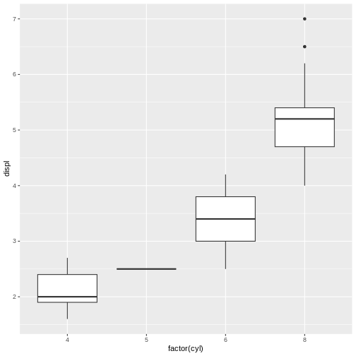
I’m working with this data about cars. The class column refers to the type of car–for example, “compact” class means that the car is quite small, while “pickup” would be a pickup truck. For each car, I also have information about the city and highway mileage, and the transmission, and the number of cylinders, as well as the displacement. This dataset has 234 rows and 11 columns, although this is an example dataset because my real dataset is much larger and has more like 500,000 rows. Anyway, in this example, I want to make a boxplot of displacement where each of the categories has its own color. But even though I set color = class here, only the outlines of the boxplots got colored in, and the inside is still white. How do I make the inside a different color? Here’s a reprex.

R

library(ggplot2)
library(dplyr)
mpg %>%
  ggplot(aes(x = class, y = displ, color = class))+
  geom_boxplot()

Help, my code isn’t working! It says I have too many elements. I made a reprex so you can see the data and the error message. I hope that’s helpful. Thank you so much!

R

library(ggplot2)
table(mpg)

ERROR

Error in table(mpg): attempt to make a table with >= 2^31 elements

As we wrap up this lesson, let’s work on adding some context for Mickey’s reprex so they’ll be ready to send it to Remy or post it online.

Discussion

Exercise 2: Adding context

Working with the person next to you, write a brief description of Mickey’s problem that they could include with their reprex when they post it online.

Make sure that the description gives a little bit of background, describes what Mickey was trying to achieve, and describes what happened instead.

When you’re done, compare notes between the groups and see if you can come up with a final reprex for Mickey!

Key Points

The reprex package makes it easy to format and share your reproducible examples.
The reprex package helps you test whether your reprex is reproducible, and also helps you prepare the reprex to share with others.
Following a certain set of steps will make your questions clearer and likelier to get answered.

Overview

Questions

Objectives

Exercise 1 (think, pair, share): When you get stuck

Exercise 2 (think, pair, share): Helping someone else

What is a reprex?

Why use a reprex?

Helpers

Rubber duck debugging

Meet Mickey, your learning companion

Prerequisites and target audience

R

R

OUTPUT

R

OUTPUT

R

OUTPUT

Overview

Questions

Objectives

Strategy 1: Interpret error messages and change function inputs

R

ERROR

R

OUTPUT

R

ERROR

Strategy 2: Read function documentation

R

R

Code first aid strategies

Exercise 1: Applying code first aid

R

ERROR

Show me the solution

R

OUTPUT

Semantic errors

R

OUTPUT

R

OUTPUT

R

R

OUTPUT

R

Exercise 2: Syntax vs. semantic errors

Show me the solution

R

OUTPUT

R

R

ERROR

R

Identifying the problem

R

ERROR

R

OUTPUT

Strategy 4: Using print() to show information

R

OUTPUT

R

OUTPUT

R

OUTPUT

Summary: Code first aid

Code first aid strategies, detailed version

Exercise 3: Isolating the problem

R

ERROR

Show me the solution

R

ERROR

R

OUTPUT

When should I prepare my code for a reprex?

Back to our analysis: Mickey tries to get unstuck

R

Strategy 4: Using `print()` to show information