All in One View
Content from Introduction
Last updated on 2026-06-05 | Edit this page
Estimated time: 90 minutes
Overview
Questions
- What is Natural Language Processing?
- Why should we learn NLP fundamentals?
- How is text different from other data?
- How can we extract structure from text?
Objectives
- Explain what is Natural Language Processing
- Enumerate relevant NLP applications
- Describe the relationship between NLP and LLMs
- Explain why NLP fundamentals are important for text processing tasks
- Enumerate basic pre-processing operations when working with text
- Extract basic properties from text using the spaCy library
What is NLP?
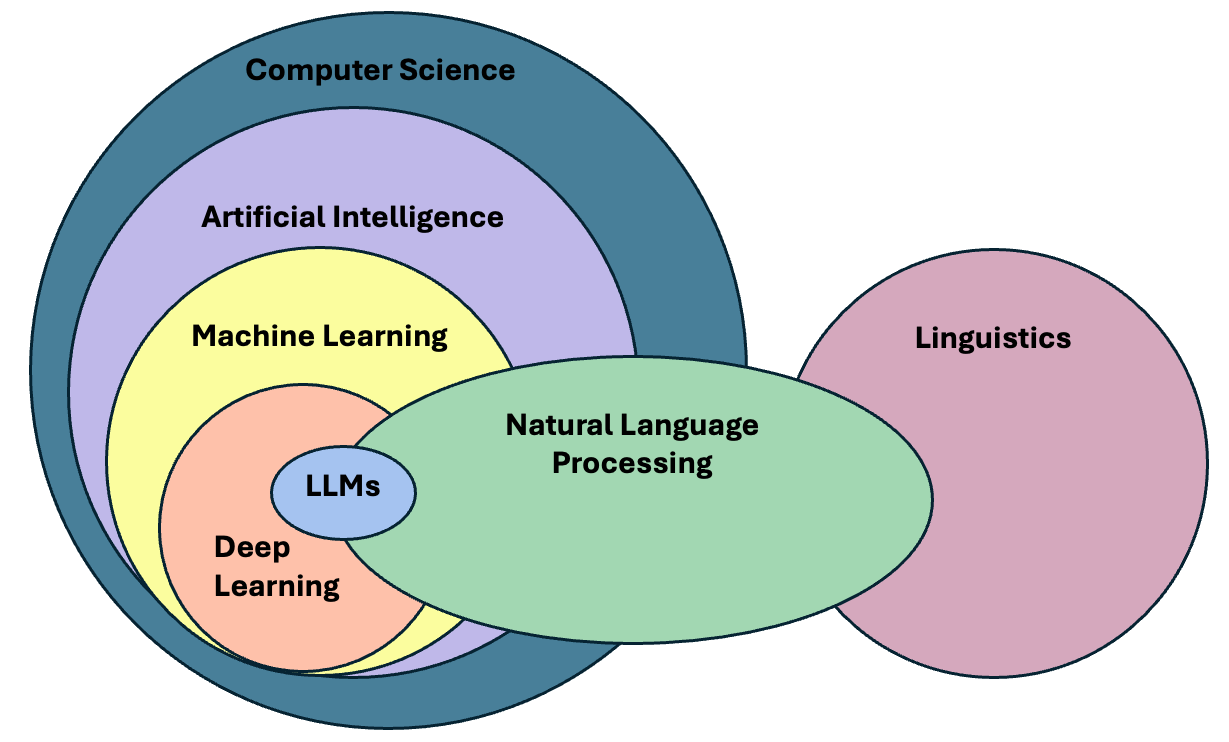
Natural language processing (NLP) is an area of research and application that focuses on making human languages processable for computers, so that they can perform useful tasks. It is therefore not a single method, but a collection of techniques that help us deal with linguistic inputs. The range of techniques spans from simple word counts, to Machine Learning (ML) methods, all the way up to complex Deep Learning (DL) architectures.
We use the term “natural language”, as opposed to “artificial language” such as programming languages, which are by design constructed to be easily formalized into machine-readable instructions. In contrast to programming languages, natural languages are complex, ambiguous, and heavily context-dependent, making them challenging for computers to process. To complicate matters, there is not only a single human language. More than 7000 languages are spoken around the world, each with its own grammar, vocabulary, and cultural context.
In this course we will mainly focus on written language, specifically written English. We leave out audio and speech, as they require a different kind of input processing. But consider that we use English only as a convenience so we can address the technical aspects of processing textual data. While ideally most of the concepts from NLP apply to most languages, one should always be aware that certain languages require different approaches to solve seemingly similar problems. We would like to encourage the usage of NLP in other less widely known languages, especially if it is a minority language. You can read more about this topic in this blogpost.
NLP in the real world
Name three to five tools/products that you use on a daily basis and that you think leverage NLP techniques. To do this exercise you may make use of the Web.
These are some of the most popular NLP-based products that we use on a daily basis:
- Agentic Chatbots (ChatGPT, Perplexity)
- Voice-based assistants (e.g., Alexa, Siri, Cortana)
- Machine translation (e.g., Google translate, DeepL, Amazon translate)
- Search engines (e.g., Google, Bing, DuckDuckGo)
- Keyboard autocompletion on smartphones
- Spam filtering
- Spell and grammar checking apps
- Customer care chatbots
- Text summarization tools (e.g., news aggregators)
- Sentiment analysis tools (e.g., social media monitoring)
We can already find differences between languages in the most basic step for processing text. Take the problem of segmenting text into meaningful units, most of the times these units are words, in NLP we call this task tokenization. A naive approach is to obtain individual words by splitting text by spaces, as it seems obvious that we always separate words with spaces. Just as human beings break up sentences into words, phrases and other units in order to learn about grammar and other structures of a language, NLP techniques achieve a similar goal through tokenization. Let’s see how can we segment or tokenize a sentence in English:
PYTHON
english_sentence = "Tokenization isn't always trivial."
english_words = english_sentence.split(" ")
print(english_words)
print(len(english_words))
OUTPUT
['Tokenization', "isn't", 'always', 'trivial.']
4
The words are mostly well separated, however we do not get fully formed words (we have punctuation with the period after “trivial” and also special cases such as the abbreviation of “is not” into “isn’t”). But at least we get a rough count of the number of words present in the sentence.
Let’s now look at the same example in Chinese:
PYTHON
# Chinese Translation of "Tokenization is not always trivial"
chinese_sentence = "标记化并不总是那么简单"

chinese_words = chinese_sentence.split(" ")
print(chinese_words)
print(len(chinese_words))
OUTPUT
['标记化并不总是那么简单']
1
The same example however did not work in Chinese, because Chinese does not use spaces to separate words. This is an example of how the idiosyncrasies of human language affects how we can process them with computers. We therefore need to use a tokenizer specifically designed for Chinese to obtain the list of well-formed words in the text. Here we use a “pre-trained” tokenizer called MicroTokenizer, which uses a dictionary-based approach to correctly identify the distinct words:
PYTHON
import MicroTokenizer  # A popular Chinese text segmentation library
chinese_sentence = "标记化并不总是那么简单"
chinese_words = MicroTokenizer.cut(chinese_sentence)
print(chinese_words)
# ['mark', 'transform', 'and', 'no', 'always', 'so', 'simple']
print(len(chinese_words))  # Output: 7
OUTPUT
['标记', '化', '并', '不', '总是', '那么', '简单']
7
We can trust that the output is valid because we are using a verified
library - MicroTokenizer, even though we don’t speak
Chinese. Another interesting aspect is that the Chinese sentence has
more words than the English one, even though they convey the same
meaning. This shows the complexity of dealing with more than one
language at a time, as is the case in task such as Machine
Translation (using computers to translate speech or text from
one human language to another).
A short history of word separation
As any historian would know, word separation in written texts is a relatively new development. You can check this yourself next time you visit a city with ancient monuments. Word separation, as oddly as it might sound today, is an example of technology.
Natural Language Processing deals with the challenges of correctly processing and generating text in any language. This can be as simple as counting word frequencies to detect different writing styles, using statistical methods to classify texts into different categories, or using deep neural networks to generate human-like text by exploiting word co-occurrences in large amounts of texts.
Why should we learn NLP Fundamentals?
In the past decade, NLP has evolved significantly, especially in the field of deep learning, to the point that it has become embedded in our daily lives. One just needs to look at the term Large Language Models (LLMs), the latest generation of NLP models, which is now ubiquitous in news media and tech products we use on a daily basis.
The term LLM now is often (and wrongly) used as a synonym of Artificial Intelligence. We could therefore think that today we just need to learn how to manipulate LLMs in order to fulfill our research goals involving textual data. The truth is that Language Modeling has always been part of the core tasks of NLP, therefore, by learning NLP you will understand better where are the main ideas behind LLMs coming from.
LLM is a blanket term for an assembly of large neural networks that are trained on vast amounts of text data with the objective of optimising for language modelling. Generative models are optimised to output human-like text, but can also used to perform other tasks. Indeed, the surprising and fascinating properties that emerge from training models at this scale allows us to solve different complex tasks such as answering elaborate questions, translating languages, solving complex problems, generating narratives that emulate reasoning, and many more. All of this with a single tool.
It is important, however, to pay attention to what is happening behind the scenes in order to trace sources of errors and biases that get hidden in the complexity of these models. The purpose of this course is precisely to take a step back and understand that:
- There are a wide variety of tools available, beyond LLMs, that do not require so much computing power
- Sometimes a much simpler method than an LLM is available that can solve our problem at hand
- If we learn how previous approaches to solve linguistic problems were designed, we can better understand the limitations of LLMs and how to use them effectively
- LLMs excel at confidently delivering information, without any regards for correctness. This calls for a careful design of evaluation metrics that give us a better understanding of the quality of the generated content.
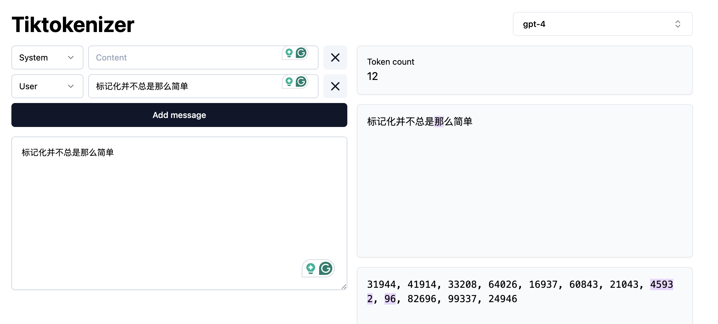
Let’s go back to our problem of segmenting text and see what ChatGPT has to say about tokenizing Chinese text:
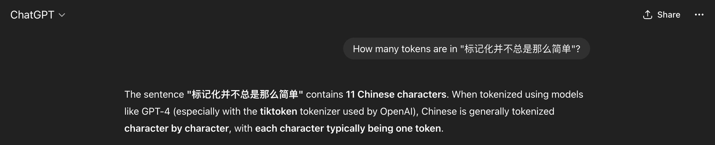
We got what sounds like a straightforward confident answer. However, it is not clear how the model arrived at this solution. Second, we do not know whether the solution is correct or not. In this case ChatGPT made some assumptions for us, such as choosing a specific kind of tokenizer to give the answer, and since we do not speak the language, we do not know if this is indeed the best approach to tokenize Chinese text. If we understand the concept of Token (which we will today!), then we can be more informed about the quality of the answer, whether it is useful to us, and therefore make a better use of the model.
And by the way, ChatGPT was almost correct, in the specific case of the gpt-4 tokenizer, the model will return 12 tokens (not 11!) for the given Chinese sentence.
We can also argue if the statement “Chinese is generally tokenized character by character” is an overstatement or not. In any case, the real question here is: Are we ok with almost correct answers? Please note that this is not a call to avoid using LLM’s but a call for a careful consideration of usage and more importantly, an attempt to explain the mechanisms behind via NLP concepts.
Language as Data
From a more technical perspective, NLP focuses on applying advanced statistical techniques to linguistic data. This is a key factor, since we need a structured dataset with a well defined set of features in order to manipulate it numerically. Your first task as an NLP practitioner is to understand what aspects of textual data are relevant for your application. Afterwards you can apply techniques to systematically extract meaningful features from unstructured data (if using statistics or Machine Learning) or choose an appropriate neural architecture (if using Deep Learning) that can help solve our problem at hand.
What is a word?
When dealing with language, our basic data unit is usually a word. We deal with sequences of words and with how they relate to each other to generate meaning in text pieces. Thus, our first step will be to load a text file and provide it with basic structure by splitting it into valid words (this is known as tokenization)!
Token vs Word
For simplicity, in the rest of the course we will use the terms “word” and “token” interchangeably, but as we just saw they do not always have the same granularity. Originally the concept of token comprised dictionary words, numeric symbols and punctuation. Nowadays, tokenization has also evolved and became an optimization task on its own (How can we segment text in a way that neural networks learn optimally from text?). Tokenizers allow one to reconstruct or revert back to the original pre-tokenized form of tokens or words, hence we can afford to use token and word as synonyms. If you are curious, you can visualize how different state-of-the-art tokenizers split text in this WebApp
Let’s open a file, read it into a string and split it by spaces. We will print the original text and the list of “words” to see how they look:
PYTHON
with open("data/84_frankenstein_or_the_modern_prometheus.txt") as f:
  text = f.read()

print(text[:150])
print("\nLength:", len(text))

print("\nProto-Tokens:")
proto_tokens = text.split(" ")
print(proto_tokens[:50])
print(len(proto_tokens))
OUTPUT
Letter 1


St. Petersburgh, Dec. 11th, 17--

TO Mrs. Saville, England

You will rejoice to hear that no disaster has accompanied the
commencement of a

Length: 421419

Proto-Tokens:
['Letter', '1\n\n\nSt.', 'Petersburgh,', 'Dec.', '11th,', '17--\n\nTO', 'Mrs.', 'Saville,', 'England\n\nYou', 'will', 'rejoice', 'to', 'hear', 'that', 'no', 'disaster', 'has', 'accompanied', 'the\ncommencement', 'of', 'an', 'enterprise', 'which', 'you', 'have', 'regarded', 'with', 'such', 'evil\nforebodings.', '', 'I', 'arrived', 'here', 'yesterday,', 'and', 'my', 'first', 'task', 'is', 'to', 'assure\nmy', 'dear', 'sister', 'of', 'my', 'welfare', 'and', 'increasing', 'confidence', 'in']
71197
Splitting by white space is possible but needs several extra steps to
get clean words as we know them. We can also use the python
split() function, which will basically strip any
whitespace-like character (including new lines) and get some
improvements:
PYTHON
print("\nProto-Tokens:")
proto_tokens = text.split()
print(proto_tokens[:50])
print(len(proto_tokens))
OUTPUT
Proto-Tokens:
['Letter', '1', 'St.', 'Petersburgh,', 'Dec.', '11th,', '17--', 'TO', 'Mrs.', 'Saville,', 'England', 'You', 'will', 'rejoice', 'to', 'hear', 'that', 'no', 'disaster', 'has', 'accompanied', 'the', 'commencement', 'of', 'an', 'enterprise', 'which', 'you', 'have', 'regarded', 'with', 'such', 'evil', 'forebodings.', 'I', 'arrived', 'here', 'yesterday,', 'and', 'my', 'first', 'task', 'is', 'to', 'assure', 'my', 'dear', 'sister', 'of', 'my']
74942
however still several extra steps are needed to separate out punctuation appropriately, and perhaps the rules become cumbersome.
Data Formatting
Texts come from various sources and are available in different formats (e.g., Microsoft Word documents, PDF documents, ePub files, plain text files, Web pages etc.). The first step is to obtain a clean text representation that can be transferred into Python UTF-8 strings that our scripts can manipulate.
Data formatting operations might include:
- Remove HTML tags (e.g., if you are extracting text from Web pages)
- Strip non-meaningful punctuation (e.g., “The quick brown fox jumps over the lazy dog and con- tinues to run across the field.)
- Strip footnotes, headers, tables, images etc.
- Remove URLs or phone numbers
- Removal of special or noisy characters (from scanned texts, for
example):
- Random symbols: “The total cost is $120.00#” → remove #
- Incorrectly recognized letters or numbers: 1 misread as l, 0 as O, etc. Example: “l0ve” → should be “love”
- Control or formatting characters: , ppearing in the middle of sentences. Example: “Pleaseform.” → “Please submit your form.”
- Non-displayable characters: �, �, or other placeholder symbols where OCR failed. Example: “Th� quick brown fox” → “The quick brown fox”
And what if you need to extract text from MS Word docs or PDF files or Web pages? There are various Python libraries for helping you extract and manipulate text from these kinds of sources.
- For MS Word documents python-docx is popular.
- For (text-based) PDF files PyPDF2 and PyMuPDF are widely used. Note that some PDF files are encoded as images (pixels) and not text. For digitizing printed text, you can use OCR (Optical Character Recognition) libraries such as pytesseract to convert the image to machine-readable text.
- For scraping text from websites, BeautifulSoup and Scrapy are some common options.
- LLMs also have something to offer here, and the field is moving pretty fast. There are some interesting open source LLM-based document parsers and OCR-like extractors such as Marker, or PyMuPDF4LLM, just to mention a couple.
The spaCy NLP Library
A more sophisticated approach to segment text files is by using specialized NLP libraries. One of the most popular is spaCy. SpaCy is a free open-source library that focuses on implementing NLP techniques to process text (in several languages, not just English) and extract insights form it in a functional and scalable fashion. Here we will start by using it to segment the text into human-readable tokens. To start, we need to download the pre-trained model, in this case we only need the small English version:
This is a model that spaCy already trained for us on a subset of web English data. Hence, the model already “knows” how to obtain clean tokens from English text. When the model processes a string, it does not only do the splitting for us but already provides more advanced linguistic properties of the tokens (such as part-of-speech tags, or named entities). You can check more languages and models in the spacy documentation.
Now we will see how spaCy help us to process text and extract interesting properties from it.
Tokenization
Tokenization is a foundational operation in NLP, as it helps to
create structure from raw text. This structure is a basic requirement
and input for modern NLP algorithms to attribute and interpret meaning
from text. This operation involves the segmentation of the text into
smaller units referred to as tokens. Tokens can be
sentences (e.g. 'the happy cat'), words
('the', 'happy', 'cat'), subwords
('un', 'happiness') or characters
('c','a', 't'). Different NLP algorithms may require
different choices for the token unit. And different languages may
require different approaches to identify or segment these tokens.
To see how tokenization works using spaCy, let’s now import the model and use it to parse our document:
PYTHON
import spacy

nlp = spacy.load("en_core_web_sm") # we load the small English model for efficiency

doc = nlp(text)
print(type(doc))  # Should be <class 'spacy.tokens.doc.Doc'>
print(len(doc)) # the length of the doc is the number of tokens
print(doc[:50]) # however if we print the doc we get the "raw" text of the first 50 tokens, not the tokens themselves
OUTPUT
<class 'spacy.tokens.doc.Doc'>
94553
Letter 1


St. Petersburgh, Dec. 11th, 17--

TO Mrs. Saville, England

You will rejoice to hear that no disaster has accompanied the
commencement of an enterprise which you have regarded with such evil
forebodings.  I arrived here yesterday
Now let’s access the tokens with spaCy and see what we get:
PYTHON
# SpaCy-Tokens
tokens = [token.text for token in doc] # Note that spacy tokens are actually python objects
print(tokens[:50])
print(len(tokens))
OUTPUT
['Letter', '1', '\n\n\n', 'St.', 'Petersburgh', ',', 'Dec.', '11th', ',', '17', '-', '-', '\n\n', 'TO', 'Mrs.', 'Saville', ',', 'England', '\n\n', 'You', 'will', 'rejoice', 'to', 'hear', 'that', 'no', 'disaster', 'has', 'accompanied', 'the', '\n', 'commencement', 'of', 'an', 'enterprise', 'which', 'you', 'have', 'regarded', 'with', 'such', 'evil', '\n', 'forebodings', '.', ' ', 'I', 'arrived', 'here', 'yesterday']
94553A good word tokenizer for example, does not simply break up a text based on spaces and punctuation, but it should be able to distinguish:
- abbreviations that include points (e.g.: e.g.)
- times (11:15) and dates written in various formats (01/01/2024 or 01-01-2024)
- word contractions such as don’t, these should be split into do and n’t
- URLs
Many older tokenizers are rule-based, meaning that they iterate over a number of predefined rules to split the text into tokens, which is useful for splitting text into word tokens for example. Modern large language models use subword tokenization, which learn to break text into pieces that are statistically convenient, this makes them more flexible but less human-readable.
The differences look subtle at the beginning, but if we carefully inspect the way spaCy splits the text, we can see the advantage of using a specialized tokenizer.
We do not have to depend necessarily on the Doc and
Token spaCy objects. Once we tokenized the text with a
spaCy model, we can extract the list of words as a list of strings and
continue our text analysis:
Text Properties
There are several useful features that spaCy provides us with, beyond word tokenization. Again, it all depends on what your requirements are. For example, we can choose to extract only symbols, or only alphanumerical tokens, and more advanced linguistic properties, for example we can remove punctuation and only keep alphanumerical tokens (or “normal words”):
PYTHON
only_words = [token for token in doc if token.is_alpha]  # Only alphanumerical tokens
print(only_words[:50])
print(len(only_words))
OUTPUT
[Letter, Petersburgh, TO, Saville, England, You, will, rejoice, to, hear, that, no, disaster, has, accompanied, the, commencement, of, an, enterprise, which, you, have, regarded, with, such, evil, forebodings, I, arrived, here, yesterday, and, my, first, task, is, to, assure, my, dear, sister, of, my, welfare, and, increasing, confidence, in, the]
75062
or keep only the verbs from our text, based on the Part-of-Speech tag that is predicted for each token:
PYTHON
only_verbs = [token for token in doc if token.pos_ == "VERB"]  # Only verbs
print(only_verbs[:10])
print(len(only_verbs))
OUTPUT
[rejoice, hear, accompanied, regarded, arrived, assure, increasing, walk, feel, braces]
10148Another important choice at the data formatting level is to decide at what granularity do you need to perform the NLP task:
- Are you analyzing phenomena at the word level? For example, detecting abusive language (based on a known vocabulary).
- Do you need to first extract sentences from the text and do analysis at the sentence level? For example, extracting entities in each sentence.
- Do you need full chunks of text? (e.g. paragraphs or chapters?) For example, summarizing each paragraph in a document.
- Or perhaps you want to extract patterns at the document level? For example each full book should have one genre tag (Romance, History, Poetry).
Sometimes your data will be already available at the desired granularity level. If this is not the case, then during the tokenization step you will need to figure out how to obtain the desired granularity level.
SpaCy also predicts the sentences under the hood for us. It might seem trivial to you as a human reader to recognize where a sentence begins and ends. But for a machine, just like finding words, finding sentences is a task on its own, for which sentence-segmentation models exist. In the case of spaCy, we can access the sentences like this:
PYTHON
sentences = [sent.text for sent in doc.sents] # Sentences are also python objects
print(sentences[:5])
print(len(sentences))
OUTPUT
['Letter 1 St. Petersburgh, Dec. 11th, 17-- TO Mrs. Saville, England You will rejoice to hear that no disaster has accompanied the commencement of an enterprise which you have regarded with such evil forebodings.', 'I arrived here yesterday, and my first task is to assure my dear sister of my welfare and increasing confidence in the success of my undertaking.', 'I am already far north of London, and as I walk in the streets of Petersburgh, I feel a cold northern breeze play upon my cheeks, which braces my nerves and fills me with delight.', 'Do you understand this feeling?', 'This breeze, which has traveled from the regions towards which I am advancing, gives me a foretaste of those icy climes.']
3317
Note that in this case each sentence is a Python object, and the
property .text returns an untokenized string (in terms of
words). But we can still access the list of word tokens inside each
sentence object if we want:
Lowercasing
Removing uppercases to e.g. avoid treating “Dog” and “dog” as two different words could also be useful, for example to train word vector representations, where we want to merge both occurrences as they represent exactly the same concept. Lowercasing can be done with Python directly as:
Beware that lowercasing the whole string as a first step might affect
the tokenizer behavior since tokenization benefits from information
provided by case-sensitive strings. We can therefore tokenize first
using spaCy and then obtain the lowercase strings of each token using
the .lower_ property:
Lemmatization
Another way to normalize words in a text is to transform them into
their dictionary form. Consider how “eating”, “ate”, “eaten”
are all variations of the root verb “eat”. Each variation is known as an
inflection of the root word. Conversely, we say that the word
“eat” is the lemma for the words “eating”, “eats”, “eaten”,
“ate” etc. Lemmatization is therefore the process of rewriting each word
in a given input text as its lemma. You can also use lemmatization for
generating word embeddings. For example, you can have a single vector
for eat instead of one vector per verb tense.
Lemmatization is not only a possible preprocessing step in NLP but
also an NLP task on its own, with different algorithms for it. Therefore
we also tend to use pre-trained models to perform lemmatization. Using
spaCy we can access the lemmmatized version of each token with the
lemma_ property (notice the underscore!):
Note that the list of lemmas is now a list of strings.
Named Entities
The default spaCy pipeline already runs more advanced tasks, such as Named Entity Recognition (NER), the task of identifying words or phrases that refer to unique real-world instances (normally proper nouns). You can access the entities with:
We can also see what named entities the model predicted based on the tokens:
OUTPUT
1713
DATE Dec. 11th
CARDINAL 17
PERSON Saville
GPE England
DATE yesterday
Note that this is a case where lowercasing your text can significantly lower the performance of your model. This is because words that start with an uppercase (not preceded by a period) usually represent proper nouns that map into Entities, for example:
PYTHON
import spacy
# Preserving uppercase characters increases the likelihood that an NER model
# will correctly identify Apple and Will as a company (ORG) and a person (PER)
# respectively.
str1 = "My next laptop will be from Apple, Will said."
# Lowercasing can reduce the likelihood of accurate labeling
str2 = "my next laptop will be from apple, will said."

nlp = spacy.load("en_core_web_sm")
ents1 = [ent.text for ent in nlp(str1).ents]
ents2 = [ent.text for ent in nlp(str2).ents]

print(ents1)
print(ents2)
OUTPUT
['Apple', 'Will']
[]Computing stats with spaCy
Use the spaCy Doc object to compute an aggregate statistic about the
Frankenstein book. HINT: Use the python set,
dictionary or Counter objects to hold the
accumulative counts. For example:
- Give the list of the 20 most common verbs in the book
- How many different Places are identified in the book? (Label = GPE)
- How many different entity categories are in the book?
- Who are the 10 most mentioned PERSONs in the book?
- Or any other similar aggregate you want…
Let’s describe the solution to obtain all the different entity categories. For that we should iterate the whole text and keep a python set with all the seen labels.
PYTHON
entity_types = set()

for ent in doc.ents:
    entity_types.add(ent.label_)

print(entity_types)
print(len(entity_types))
OUTPUT
{'CARDINAL', 'GPE', 'WORK_OF_ART', 'ORDINAL', 'DATE', 'LAW', 'PRODUCT', 'QUANTITY', 'ORG', 'TIME', 'PERSON', 'LOC', 'LANGUAGE', 'FAC', 'NORP'}
15NLP Libraries
Related to the need of shaping our problems into a known task, there
are several existing NLP libraries which provide a wide range of models
that we can use out-of-the-box (without further need of modification).
We already saw simple examples using spaCy for English and
MicroTokenizer for Chinese. Again, as a non-exhaustive
list, we mention some widely used NLP libraries in Python:
What did we learn in this lesson?
- NLP is a subfield of Articifial Intelligence that, with help from Linguistics, deals with processing, understanding, and generating natural language data.
- Linguistic data has unique properties that make it challenging to process computationally: it is unstructured, ambiguous, context-dependent, and varies significantly across the 7000+ human languages.
- Tokenization is the foundational step in NLP: splitting text into meaningful units (tokens) creates the structure that all downstream algorithms require.
- Language Modeling is a subset of NLP, not a synonym for AI: understanding NLP fundamentals (tokenization, statistical models, evaluation, …) can help to trace errors, detect biases, and use LLMs more critically and effectively.
- Text pre-processing is a pipeline of decisions: character cleaning, tokenization, lowercasing, and lemmatizing are common steps that can be used to improve the performance of your task.
- Libraries like spaCy are very light and make it practical to extract linguistic features (tokens, lemmas, part-of-speech tags, named entities, and sentence boundaries) from text in different languages with minimal code.
Content from A Primer on Linguistics
Last updated on 2026-05-20 | Edit this page
Estimated time: 60 minutes
Overview
Questions
- How is language approached from a Machine Learning perspective?
- What does it mean to do Language Modeling?
- What linguistic properties should we consider when dealing with texts?
Objectives
- Identify the most relevant existing NLP tasks
- Describe what the Language Modeling task is
- Explain why automatic processing of language is difficult
- Demonstrate linguistic concepts by coding short examples with text data
Natural language exhibits a set of properties that make it more challenging to process than other types of data such as tables, spreadsheets or time series. To address this, we can first visit the existing different ways of abstracting the problems when dealing with texts. This is what is called an NLP task: deciding on the important aspects that interest us in a the text and how to extract them. We will then revisit basic linguistic concepts that make text processing difficult in general. Language is hard to process because it is compositional, ambiguous, discrete and sparse. Let’s visit each of these concepts and understand them.
NLP tasks
There are several ways to describe the tasks that NLP solves. From the Machine Learning perspective, we have:
- Unsupervised tasks: exploiting existing patterns from large amounts of text.
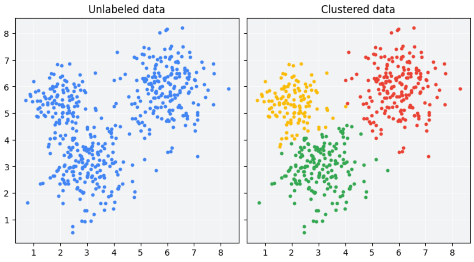
- Supervised tasks: learning to classify texts given a labeled set of examples
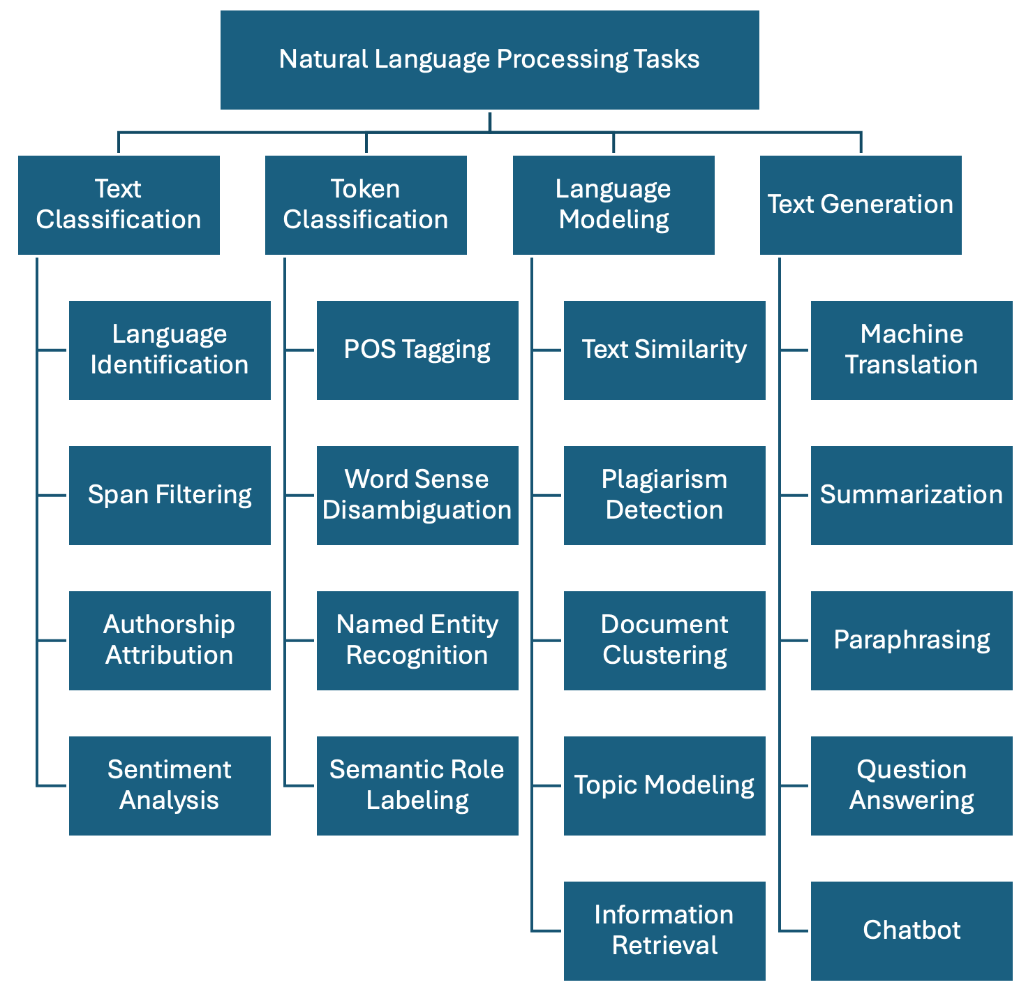
Regardless of the chosen method, we show one possible taxonomy of NLP tasks below. The tasks are grouped together with some of their most prominent applications. This is a non-exhaustive list, as in reality there are hundreds of them, but it is a good start:
-
Text Classification: Assign one or more labels to a given piece of text. This text is usually referred to as a document and in our context this can be a sentence, a paragraph, a book chapter, etc…
- Language Identification: determining the language in which a particular input text is written.
- Spam Filtering: classifying emails into spam or not spam based on their content.
- Authorship Attribution: determining the author of a text based on its style and content (based on the assumption that each author has a unique writing style).
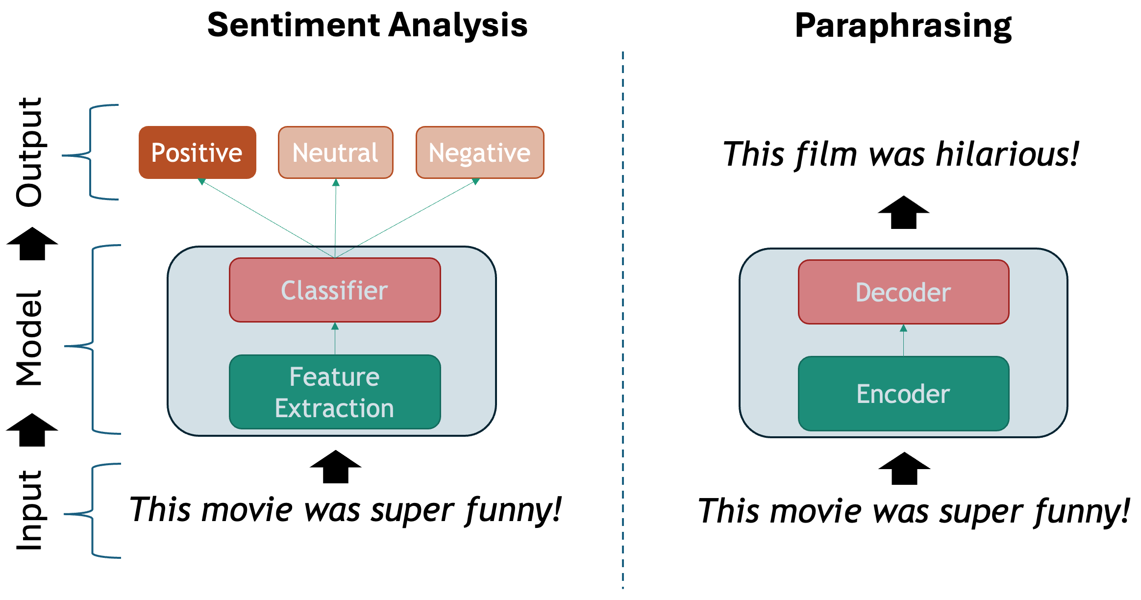
- Sentiment Analysis: classifying text into positive, negative or neutral sentiment. For example, in the sentence “I love this product!”, the model would classify it as positive sentiment.
-
Token Classification: The task of individually assigning one label to each word in a document. This is a one-to-one mapping; however, because words do not occur in isolation and their meaning depend on the sequence of words to the left or the right of them, this is also called Word-In-Context Classification or Sequence Labeling and usually involves syntactic and semantic analysis.
- Part-Of-Speech Tagging: is the task of assigning a part-of-speech label (e.g., noun, verb, adjective) to each word in a sentence.
- Chunking: splitting a running text into “chunks” of words that together represent a meaningful unit: phrases, sentences, paragraphs, etc.
- Word Sense Disambiguation: based on the context what does a word mean (think of “book” in “I read a book.” vs “I want to book a flight.”)
- Named Entity Recognition: recognize world entities in text, e.g. Persons, Locations, Book Titles, or many others. For example “Mary Shelley” is a person, “Frankenstein or the Modern Prometheus” is a book, etc.
- Semantic Role Labeling: the task of finding out “Who did what to whom?” in a sentence: information from events such as agents, participants, circumstances, subject-verb-object triples etc.
- Relation Extraction: the task of identifying named relationships between entities in a text, e.g. “Apple is based in California” has the relation (Apple, based_in, California).
- Co-reference Resolution: the task of determining which words refer to the same entity in a text, e.g. “Mary is a doctor. She works at the hospital.” Here “She” refers to “Mary”.
- Entity Linking: the task of disambiguation of named entities in a text, linking them to their corresponding entries in a knowledge base, e.g. Mary Shelley’s biography in Wikipedia.
-
Language Modeling: Given a sequence of words, the model predicts the next word. For example, in the sentence “The capital of France is _____”, the model should predict “Paris” based on the context. This task was initially useful for building solutions that require speech and optical character recognition (even handwriting), language translation and spelling correction. Nowadays this has scaled up to the LLMs that we know. A byproduct of pre-trained Language Modeling is the vectorized representation of texts which allows to perform specific tasks such as:
- Text Similarity: The task of determining how similar two pieces of text are.
- Plagiarism detection: determining whether a piece of text, B, is close enough to another known piece of text, A, which increases the likelihood that it was plagiarized.
- Document clustering: grouping similar texts together based on their content.
- Topic modelling: a specific instance of clustering, here we automatically identify abstract “topics” that occur in a set of documents, where each topic is represented as a cluster of words that frequently appear together.
- Information Retrieval: this is the task of finding relevant information or documents from a large collection of unstructured data based on user’s query, e.g., “What’s the best restaurant near me?”.
-
Text Generation: the task of generating text based on a given input. This is usually done by generating the output word by word, conditioned on both the input and the output so far. The difference with Language Modeling is that for generation there are higher-level generation objectives such as:
- Machine Translation: translating text from one language to another, e.g., “Hello” in English to “Que tal” in Spanish.
- Summarization: generating a concise summary of a longer text. It can be abstractive (generating new sentences that capture the main ideas of the original text) but also extractive (selecting important sentences from the original text).
- Paraphrasing: generating a new sentence that conveys the same meaning as the original sentence, e.g., “The cat is on the mat.” to “The mat has a cat on it.”.
- Question Answering: given a question and a context, the model generates an answer. For example, given the question “What is the capital of France?” and the Wikipedia article about France as the context, the model should answer “Paris”. This task can be approached as a text classification problem (where the answer is one of the predefined options) or as a generative task (where the model generates the answer from scratch).
- Conversational Agent (ChatBot): Building a system that interacts with a user via natural language, e.g., “What’s the weather today, Siri?”. These agents are widely used to improve user experience in customer service, personal assistance and many other domains.
Compositionality
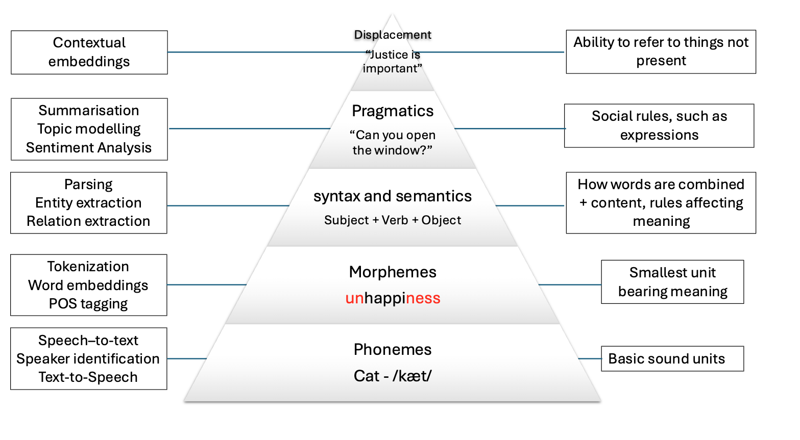
The basic elements of written languages are characters, a sequence of characters form words, and words in turn denote objects, concepts, events, actions and ideas (Goldberg, 2016). Subsequently, words form phrases and sentences which are used in communication and depend on the context in which they are used. We as humans derive the meaning of utterances from interpreting contextual information that is present at different levels at the same time:

The first two levels refer to spoken language only, and the other four levels are present in both speech and text. Because in principle machines do not have access to the same levels of information that we do (they can only have independent audio, textual or visual inputs), we need to come up with clever methods to overcome this significant limitation. Knowing the levels of language is important so we consider what kind of problems we are facing when attempting to solve our NLP task at hand.
Ambiguity
The disambiguation of meaning is usually a by-product of the context in which utterances are expressed and also of the historic accumulation of interactions which are transmitted across generations (think for instance to idioms – these are usually meaningless phrases that acquire meaning only if situated within their historical and societal context). These characteristics make NLP a particularly challenging field to work in.
We cannot expect a machine to process human language and simply understand it as it is. We need a systematic, scientific approach to deal with it. It’s within this premise that the field of NLP is born, primarily interested in converting the building blocks of human/natural language into something that a machine can understand.
The image below shows how the levels of language relate to a few NLP applications:
Levels of ambiguity
Discuss what the following sentences mean. What level of ambiguity do they represent?:
“The door is unlockable from the inside.” vs “Unfortunately, the cabinet is unlockable, so we can’t secure it”
“I saw the cat with the stripes” vs “I saw the cat with the telescope”
“Please don’t drive the cat to the vet!” vs “Please don’t drive the car tomorrow!”
“I never said she stole my money.” (re-write this sentence multiple times and each time emphasize a different word in uppercases).
This is why the previous statements were difficult:
- “Un-lockable vs Unlock-able” is a Morphological ambiguity: Same word form, two possible meanings
- “I saw the cat with the telescope” has a Syntactic ambiguity: Same sentence structure, different properties
- “drive the cat” vs “drive the car” shows a Semantic ambiguity: Syntactically identical sentences that imply quite different actions.
- “I NEVER said she stole MY money.” is a Pragmatic ambiguity: Meaning relies on word emphasis
Whenever you are solving a specific task, you should ask yourself what kind of ambiguity can affect your results, and to what degrees? At what level are your assumptions operating when defining your research questions? Having the answers to this can save you a lot of time when debugging your models. Sometimes the most innocent assumptions (for example using the wrong tokenizer) can create enormous performance drops even when the higher level assumptions were correct.
Sparsity
Another key property of linguistic data is its sparsity. This means that if we are hunting for a specific phenomenon, we may often realize it barely occurs inside a vast amount of text. Imagine we have the following brief text and we are interested in pizzas and hamburgers:
PYTHON
# A mini-corpus where our target words appear
text = """
I am hungry. Should I eat delicious pizza?
Or maybe I should eat a juicy hamburger instead.
Many people like to eat pizza because is tasty, they think pizza is delicious as hell!
My friend prefers to eat a hamburger and I agree with him.
We will drive our car to the restaurant to get the succulent hamburger.
Right now, our cat sleeps on the mat so we won't take him.
I did not wash my car, but at least the car has gasoline.
Perhaps when we come back we will take out the cat for a walk.
The cat will be happy then.
"""
We can first use spaCy to tokenize the text and do some direct word count:
PYTHON
import spacy
nlp = spacy.load("en_core_web_sm")

doc = nlp(text)
words = [token.lower_ for token in doc if token.is_alpha]  # Filter out punctuation and new lines
print(words)
print(len(words))
We have in total 104 words, but we actually want to know how many times each word appears. For that we use the Python Counter and then we can visualize it inside a chart with matplotlib:
PYTHON
from collections import Counter
import matplotlib.pyplot as plt

word_count = Counter(words).most_common()
tokens = [item[0] for item in word_count]
frequencies = [item[1] for item in word_count]

plt.figure(figsize=(18, 6))
plt.bar(tokens, frequencies)
plt.xticks(rotation=90)
plt.show()
This bar chart shows us several things about sparsity, even with such a small text:
The most common words are filler words such as “the”, “of”, “not” etc. These are known as stopwords because such words by themselves generally do not hold a lot of information about the meaning of the piece of text.
The two concepts (hamburger and pizza) we are interested in, appear only 3 times each, out of 104 words (comprising only ~3% of our corpus). This number only goes lower as the corpus size increases
There is a long tail in the distribution, where actually a lot of meaningful words are located.
Stop Words
The most frequent words in texts are those which contribute little semantic value on their own: articles (‘the’, ‘a’, ‘an’), conjunctions (‘and’, ‘or’, ‘but’), prepositions (‘on’, ‘by’), auxiliary verbs (‘is’, ‘am’), pronouns (‘he’, ‘which’), or any highly frequent word that might not be of interest in several content-only related tasks.
Stop words are extremely frequent syntactic filler words that not always provide relevant semantic information for our use case. For some use cases it is better to ignore them in order to fight the sparsity phenomenon. However, consider that in many other use cases the syntactic information that stop words provide is crucial to solve the task.
SpaCy has a pre-defined list of stopwords per language. To explicitly load the English stop words we can do:
PYTHON
from spacy.lang.en.stop_words import STOP_WORDS
print(STOP_WORDS)  # a set of common stopwords
print(len(STOP_WORDS)) # There are 326 words considered in this list
You can also manually extend the list of stop words if you are interested in ignoring other unlisted terms that you encounter in your data.
Alternatively, you can filter out stop words when iterating your tokens (remember the spaCy token properties!) like this:
PYTHON
doc = nlp(text)
content_words = [token.text for token in doc if token.is_alpha and not token.is_stop]  # Filter out stop words and punctuation
print(content_words)
There is no canonical definition of stop words because what you consider to be a stop word is directly linked to the objective of your task at hand. For example, pronouns are usually considered stopwords, but if you want to do gender bias analysis then pronouns are actually a key element of your text processing pipeline. Similarly, removing articles and prepositions from text is obviously not advised if you are doing dependency parsing (the task of identifying the parts of speech in a given text).
Another special case is the word ‘not’ which may encode the semantic notion of negation. Removing such tokens can drastically change the meaning of sentences and therefore affect the accuracy of models for which negation is important to preserve (e.g., sentiment classification “this movie was NOT great” vs. “this movie was great”).
Sparsity is closely related to what is frequently called domain-specific data. The discourse context in which language is used varies importantly across disciplines (domains). Take for example law texts and medical texts which are typically filled with domain-specific jargon. We should expect the top part of the distribution to contain mostly the same words as they tend to be stop words. But once we remove the stop words, the top of the distribution will contain very different content words.
Also, the meaning of concepts described in each domain might significantly differ. For example the word “trial” refers to a procedure for examining evidence in court, but in the medical domain this could refer to a clinical “trial” which is a procedure to test the efficacy and safety of treatments on patients. For this reason there are specialized models and corpora that model language use in specific domains. The concept of fine-tuning a general purpose model with domain-specific data is also popular, even when using LLMs.
Discreteness
There is no inherent relationship between the form of a word and its meaning. For this reason, by syntactic or lexical analysis alone, there is no automatic way of knowing if two words are similar in meaning or how they relate semantically to each other. For example, “car” and “cat” appear to be very closely related at the morphological level, only one letter needs to change to convert one word into the other. But the two words represent concepts or entities in the world which are very different. Conversely, “pizza” and “hamburger” look very different (they only share one letter in common) but are more closely related semantically, because they both refer to typical fast foods.
How can we automatically know that “pizza” and “hamburger” share more semantic properties than “car” and “cat”? One way is by looking at the context (neighboring words) of these words. This idea is the principle behind distributional semantics, and aims to look at the statistical properties of language, such as word co-occurrences (what words are typically located nearby a given word in a given corpus of text), to understand how words relate to each other.
Let’s keep using the list of words from our mini corpus:
Now we will create a dictionary where we accumulate the words that appear around our words of interest. In this case we want to find out, according to our corpus, the most frequent words that occur around pizza, hamburger, car and cat:
PYTHON
target_words = ["pizza", "hamburger", "car", "cat"] # words we want to analyze
co_occurrence = {word: [] for word in target_words}
co_occurrence
We iterate over each word in our corpus, collecting its surrounding
words within a defined window. A window consists of a set number of
words to the left and right of the target word, as determined by the
window_size parameter. For example, with window_size = 3, a
word W has a window of six neighboring words—three
preceding and three following—excluding W itself:
PYTHON
window_size = 3 # How many words to look at on each side
for i, word in enumerate(words):
    # If the current word is one of our target words...
    if word in target_words:
        start = max(0, i - window_size) # get the start index of the window
        end = min(len(words), i + 1 + window_size) # get the end index of the window
        context = words[start:i] + words[i+1:end]  # Exclude the target word itself
        co_occurrence[word].extend(context)

print(co_occurrence)
We call the words that fall inside this window the
context of a target word. We can already see other
interesting related words in the context of each target word, but a lot
of non interesting stuff is in there. To obtain even nicer results, we
can delete the stop words from the context window before adding it to
the dictionary. You can define your own stop words, here we use the
STOP_WORDS list provided by spaCy:
PYTHON
from spacy.lang.en.stop_words import STOP_WORDS

co_occurrence = {word: [] for word in target_words} # Empty the dictionary

window_size = 3 # How many words to look at on each side
for i, word in enumerate(words):
    # If the current word is one of our target words...
    if word in target_words:
        start = max(0, i - window_size) # get the start index of the window
        end = min(len(words), i + 1 + window_size) # get the end index of the window
        context = words[start:i] + words[i+1:end]  # Exclude the target word itself
        context = [w for w in context if w not in STOP_WORDS] # Filter out stop words
        co_occurrence[word].extend(context)

print(co_occurrence)
Our dictionary keys represent each word of interest, and the values are a list of the words that occur within window_size distance of the word. Now we use a Counter to get the most common items:
PYTHON
# Print the most common context words for each target word
print("Contextual Fingerprints:\n")
for word, context_list in co_occurrence.items():
    # We use Counter to get a frequency count of context words
    fingerprint = Counter(context_list).most_common(5)
    print(f"'{word}': {fingerprint}")
OUTPUT
Contextual Fingerprints:

'pizza': [('eat', 2), ('delicious', 2), ('tasty', 2), ('maybe', 1), ('like', 1)]
'hamburger': [('eat', 2), ('juicy', 1), ('instead', 1), ('people', 1), ('agree', 1)]
'car': [('drive', 1), ('restaurant', 1), ('wash', 1), ('gasoline', 1)]
'cat': [('walk', 2), ('right', 1), ('sleeps', 1), ('happy', 1)]
As our mini experiment demonstrates, discreteness can be combatted with statistical co-occurrence: words with similar meaning will occur around similar concepts, giving us an idea of similarity that has nothing to do with syntactic or lexical form of words. This is the core idea behind most modern semantic representation models in NLP.
Linguistic Resources
There are also several curated resources (textual data) that can help solve your NLP-related tasks, specifically when you need highly specialized definitions. An exhaustive list would be impossible as there are thousands of them, and also them being language and domain dependent. Below we mention some of the most prominent, just to give you an idea of the kind of resources you can find, so you don’t need to reinvent the wheel every time you start a project:
- HuggingFace Datasets: A large collection of datasets for NLP tasks, including text classification, question answering, and language modeling.
- WordNet: A large lexical database of English, where words are grouped into sets of synonyms (synsets) and linked by semantic relations.
- Europarl: A parallel corpus of the proceedings of the European Parliament, available in 21 languages, which can be used for machine translation and cross-lingual NLP tasks.
- Universal Dependencies: A collection of syntactically annotated treebanks across 100+ languages, providing a consistent annotation scheme for syntactic and morphological properties of words, which can be used for cross-lingual NLP tasks.
- PropBank: A corpus of texts annotated with information about basic semantic propositions, which can be used for English semantic tasks.
- FrameNet: A lexical resource that provides information about the semantic frames that underlie the meanings of words (mainly verbs and nouns), including their roles and relations.
- BabelNet: A multilingual lexical resource that combines WordNet and Wikipedia, providing a large number of concepts and their relations in multiple languages.
- Wikidata: A free and open knowledge base initially derived from Wikipedia, that contains structured data about entities, their properties and relations, which can be used to enrich NLP applications.
- Dolma: An open dataset of 3 trillion tokens from a diverse mix of clean web content, academic publications, code, books, and encyclopedic materials, used to train English large language models.
What did we learn in this lesson?
- NLP tasks can be approached as supervised (learning from labeled examples), semi-supervised (learning from text tokens), or unsupervised (exploiting patterns in raw text).
- The main families of NLP tasks are text classification, token classification, language modeling, and text generation.
- Language is compositional: meaning is built layer by layer from
words to sentences to discourse, and sometimes more than two layers are
needed in order to describe the meaning of a piece of text.
- Language is ambiguous at multiple levels and resolving this ambiguity requires contextual information that is challenging for machines to capture.
- Language is sparse: words of interest typically appear rarely in a corpus, dominated by high-frequency stopwords that carry little semantic content.
- Language is discrete: word form does not reflect meaning: “car” and “cat” differ by one letter yet are unrelated, while “pizza” and “hamburger” look very different but are semantically more similar.
- Domain-specific language shifts the distribution of meaningful words and can change the meaning of terms entirely (e.g., “trial” in law vs. “trial” in medicine).
Content from From words to vectors
Last updated on 2026-05-22 | Edit this page
Estimated time: 120 minutes
Overview
Questions
- What are the steps that matter for defining an NLP task?
- How can words be represented as numbers that capture meaning?
- What kinds of semantic relationships can word embeddings encode?
- What are the limitations of static word representations like Word2Vec?
- How can we train our own Word2Vec model?
- How can we automatically discover hidden topics in a collection of texts?
Objectives
After following this lesson, learners will be able to:
- Implement a basic NLP Pipeline.
- Explain the motivation for vectorisation in modern NLP.
- Describe the kinds of semantic relationships captured by Word2Vec.
- Explain the limitations of the Word2Vec representation by way of example.
- Train a custom Word2Vec model using the Gensim library.
- Apply Topic Modelling to a text corpus using BERTopic.
Setup
If you haven’t done it already during the workshop setup, please run
invoke download-litbank to download the data that we are
going to use for this episode.
Introduction
In this episode, we will learn about the importance of preprocessing text in NLP, and how to apply common preprocessing operations to text files. We will also learn more about NLP Pipelines, learn about their basic components and how to construct such pipelines.
We will then address the transition from rule-based NLP to distributional semantics approaches which encode text into numerical representations based on statistical relationships between tokens. We will introduce one particular algorithm for this kind of encoding called Word2Vec, which was proposed in 2013 by Mikolov et al. We will show what kind of useful semantic relationships these representations encode in text, and how we can use them to solve specific NLP tasks. We will also discuss some of the limitations of Word2Vec which are addressed in the next lesson on transformers before concluding with a summary of what we covered in this lesson.
NLP Pipeline
The concept of NLP pipeline refers to the sequence of operations that we apply to our data in order to go from the original data (e.g. original raw documents) to the expected outputs of our NLP task at hand. The components of the pipeline refer to any manipulation we apply to the text, and do not necessarily need to be complex models. They involve preprocessing operations, application of rules or machine learning models, as well as formatting the outputs in a desired way.
A simple rule-based classifier
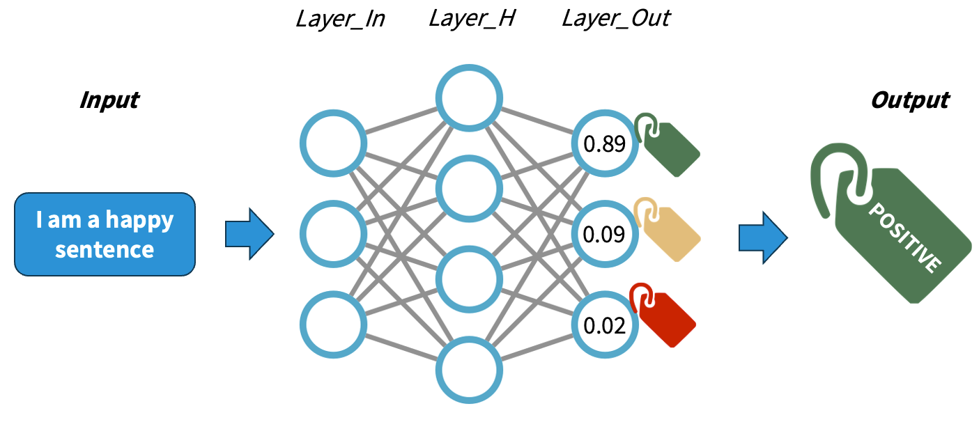
Imagine that we want to build a very lightweight sentiment classifier. A basic approach is to design the following pipeline:
- Clean the original text file (as we saw in the Data Formatting section)
- Apply a sentence segmentation or tokenisation model
- Define a set of positive and negative words (a hardcoded dictionary)
- For each sentence:
- If it contains one or more of the positive words, classify as
POSITIVE - If it contains one or more of the negative words, classify as
NEGATIVE - Otherwise classify as
NEUTRAL
- If it contains one or more of the positive words, classify as
- Output a table with the original sentence and the assigned label
This is implemented with the following code:
- Read the text and normalise it into a single line
PYTHON
import spacy
nlp = spacy.load("en_core_web_sm")

filename = "data/84_frankenstein_or_the_modern_prometheus.txt"
with open(filename, 'r', encoding='utf-8') as file:
    text = file.read()

text = text.replace("\n", " ") # some cleaning by removing new line characters- Apply sentence segmentation
- Define the positive and negative words you care about:
PYTHON
positive_words = ["happy", "excited", "delighted", "content", "love", "enjoyment"]
negative_words = ["unhappy", "sad", "anxious", "miserable", "fear", "horror"]- Apply the rules to each sentence and collect the labels
PYTHON
classified_sentences = []

for sent in sentences:
    if any(word in sent.lower() for word in positive_words):
        classified_sentences.append((sent, 'POSITIVE'))
    elif any(word in sent.lower() for word in negative_words):
        classified_sentences.append((sent, 'NEGATIVE'))
    else:
classified_sentences.append((sent, 'NEUTRAL'))- Save the classified data
PYTHON
import pandas as pd
df = pd.DataFrame(classified_sentences, columns=['sentence', 'label'])
df.to_csv('results_naive_rule_classifier.csv', sep='\t')
Challenge
Discuss the pros and cons of the proposed NLP pipeline:
- Do you think it will give accurate results?
- What do you think about the coverage of this approach? What cases will it miss?
- Think of possible drawbacks of chaining components in a pipeline.
- This classifier only considers the presence of one word to apply a label. It does not analyze sentence semantics or even syntax.
- Given how the rules are defined, if both positive and negative words
are present in the same sentence it will assign the
POSITIVElabel. It will generate a lot of false positives because of the simplistic rules. - The errors from previous steps get carried over to the next steps increasing the likelihood of noisy outputs.
So far, we’ve seen how to format and segment the text to have atomic data at the word level or sentence level. We then apply operations to the word and sentence strings. This approach still depends on counting and exact keyword matching. And as we have already seen it has several limitations. The method cannot interpret words outside the dictionary defined for example.
One way to combat this is by transforming each word into numeric representation and study statistical patterns in how these words are distributed in text. For example, what words tend to occur “close” to a given word in my data? For example, if we analyze restaurant menus we find that “cheese”, “mozzarella”, “base” etc. frequently occur near the token “pizza”. We can then exploit these statistical patterns to inform various NLP tasks. This concept is commonly known as distributional semantics. It is based on the assumption “words that appear in similar contexts have similar meanings.”
This concept is powerful for enabling, for example, the measurement of semantic similarity of words, sentences, phrases etc. in text. And this, in turn, can help with other downstream NLP tasks, as we shall see in the next section on word embeddings.
Word Embeddings
Reminder: Neural Networks
Understanding how neural networks (NNs) work is out of the scope of this course. For our purposes, we will simplify the explanation in order to conceptually understand how NNs work. A NN is a pattern-finding machine with layers (a deep NN is the same concept but scaled to dozens or even hundreds of layers). In a NN, each layer has several interconnected neurons, each one corresponding to a random number initially. The deeper the network is, the more complex patterns it can learn. As the NN gets trained (that is, as it sees several labelled examples that we provide), each neuron value will be updated in order to maximise the probability of getting the answers right. A well-trained NN will be able to predict the right labels on completely new data with a certain accuracy.
The main difference with traditional machine learning models is that we do not need to design explicitly any features, rather the network will adjust itself by looking at the data alone and executing the back-propagation algorithm. The main job when using NNs is to encode our data properly so it can be fed into the network.
Rationale behind Embeddings
A word embedding is a numeric vector that represents a word. Word2Vec exploits the “feature-agnostic” power of NNs to transform word strings into trained word numeric representations. Hence we still use words as features but instead of using the string directly, we transform that string into its corresponding vector in the pre-trained Word2Vec model. And because both the network input and output are the words themselves in text, we basically have billions of labeled training datapoints for free.
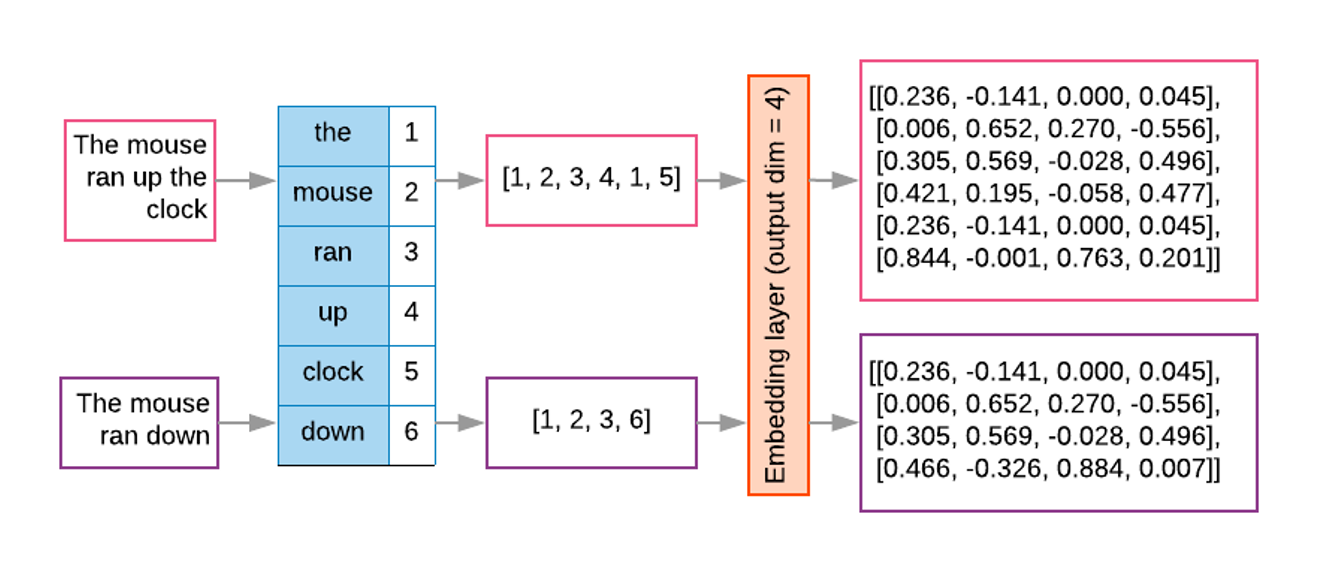
To obtained the word embeddings, a shallow NN is optimised with the task of language modeling. The final hidden layer inside the trained network holds the fixed-size vectors whose values can be mapped into linguistic properties (since the training objective was language modeling). Since similar words occur in similar contexts, or have same characteristics, a properly trained model will learn to assign similar vectors to similar words.
By representing words with vectors, we can mathematically manipulate them through vector arithmetic and express semantic similarity in terms of vector distance. Because the size of the learned vectors is not proportional to the amount of documents we can learn the representations from larger collections of texts, obtaining more robust representations, that are less corpus-dependent.
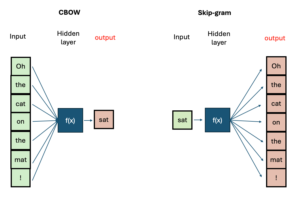
There are two main algorithms for training Word2Vec:
- Continuous Bag-of-Words (CBOW): Predicts a target word based on its surrounding context words.
- Continuous Skip-Gram: Predicts surrounding context words given a target word.
If you want to know more about the technical aspects of training Word2Vec, you can visit this tutorial
The Word2Vec Vector Space
The python package gensim offers a user-friendly
interface to interact with pre-trained Word2vec models and also to train
our own. First, we will explore the model from the original Word2Vec
paper, which was trained on a big corpus from Google News (English news
articles). We will see what functionalities are available to explore a
vector space. Then, we will prepare our own text step-by-step to train
our own Word2vec models and save them.
Load the embeddings and inspect them
The gensim package has a repository with pre-trained
English models. We can take a look at the models:
PYTHON
import gensim.downloader
available_models = gensim.downloader.info()['models'].keys()
print(list(available_models))
We will download the Google News model with:
We can do some basic checks, such as showing how many words are in the vocabulary (i.e., for how many words do we have an available vector), what is the total number of dimensions in each vector, and print the components of a vector for a given word:
PYTHON
print(len(w2v_model.key_to_index.keys())) # 3 million words
print(w2v_model.vector_size) # 300 dimensions. This can be chosen when training your own model
print(w2v_model['car'][:10]) # The first 10 dimensions of the vector representing 'car'.
print(w2v_model['cat'][:10]) # The first 10 dimensions of the vector representing 'cat'.
OUTPUT
3000000
300
[ 0.13085938  0.00842285  0.03344727 -0.05883789  0.04003906 -0.14257812
  0.04931641 -0.16894531  0.20898438  0.11962891]
[ 0.0123291   0.20410156 -0.28515625  0.21679688  0.11816406  0.08300781
  0.04980469 -0.00952148  0.22070312 -0.12597656]
As we can see, this is a very large model with 3 million words, and the dimensionality chosen at training time was 300. Therefore, each word will have a 300-dimensional vector associated with it.
However, we can always find a word that is not contained even in a very large vocabulary:
This will throw a KeyError as the model does not know
that word. Unfortunately, this is a limitation of Word2vec - unseen
words (words that were not included in the training data) cannot be
interpreted by the model.
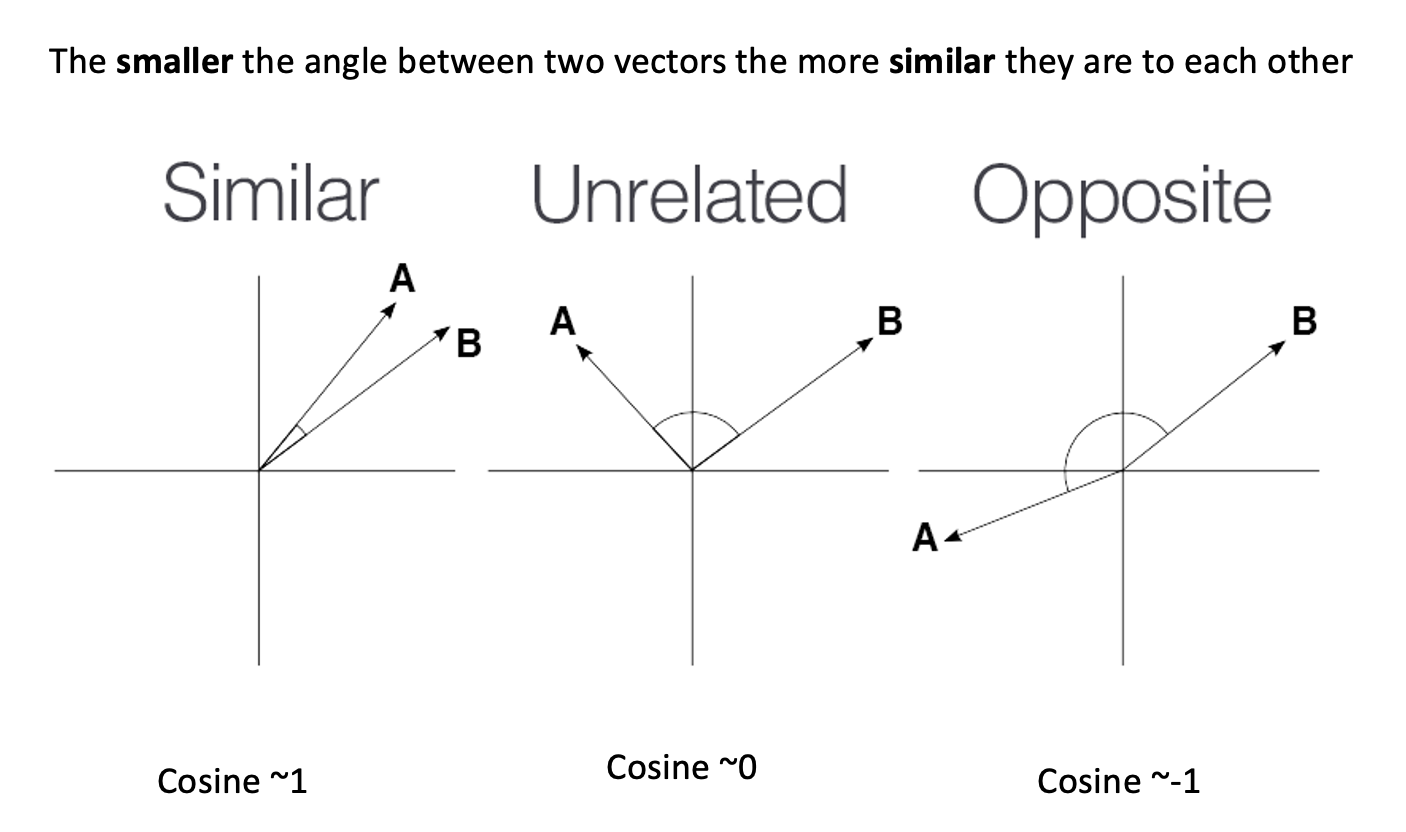
Now, let’s talk about the vectors themselves. They are not easy to interpret as they are a bunch of floating point numbers. These are the weights that the network learned when optimising for language modelling. As the vectors are hard to interpret, we rely on a mathematical method to compute how similar two vectors are. Generally speaking, the recommended metric for measuring similarity between two high-dimensional vectors is cosine similarity .
cosine
similarity ranges between [-1 and 1]. It
is the cosine of the angle between two vectors, divided by the product
of their lengths. Mathematically speaking, when two vectors point in
exactly the same direction, their cosine similarity will be 1, and when
they point in the opposite directions, their cosine similarity will be
-1. In Python, we can use SKLearn to compute the cosine similarity of
vectors.
We can use sklearn learn to measure any pair of
high-dimensional vectors:
PYTHON
from sklearn.metrics.pairwise import cosine_similarity

car_vector = w2v_model['car']
cat_vector = w2v_model['cat']

similarity = cosine_similarity([car_vector], [cat_vector])
print(f"Cosine similarity between 'car' and 'cat': {similarity[0][0]}")

similarity = cosine_similarity([w2v_model['hamburger']], [w2v_model['pizza']])
print(f"Cosine similarity between 'hamburger' and 'pizza': {similarity[0][0]}")
PYTHON
Cosine similarity between 'car' and 'cat': 0.21528185904026031
Cosine similarity between 'hamburger' and 'pizza': 0.6153676509857178
Or you can use directly the
w2v_model.similarity('car', 'cat') function which gives the
same result.
The higher similarity score between the hamburger and pizza indicates they are more similar based on the contexts where they appear in the training data. Even though is hard to read all the floating numbers in the vectors, we can trust this metric to give us a hint of which words are semantically closer than others.
Challenge
Think of different word pairs and try to guess how close or distant they will be from each other. Use the similarity measure from the Word2Vec module to compute the metric and discuss if this fits your expectations. If not, can you come up with a reason why this was not the case?
Some interesting cases include synonyms, antonyms and morphologically related words:
PYTHON
print(w2v_model.similarity('democracy', 'democratic'))
print(w2v_model.similarity('queen', 'princess'))
print(w2v_model.similarity('love', 'hate')) #!! (think of "I love X" and "I hate X")
print(w2v_model.similarity('love', 'lover'))
OUTPUT
0.86444813
0.7070532
0.6003957
0.48608577
Vector Neighborhoods
Now that we have a metric we can trust, we can retrieve neighborhoods
of vectors that are close to a given word. This is analogous to
retrieving semantically related terms to a target term. Let’s explore
the neighborhood around `pizza` using the most_similar()
method:
This returns a list of ranked tuples with the form (word, similarity_score). The list is already sorted in descending order, so the first element is the closest vector in the vector space, the second element is the second closest word, and so on.
OUTPUT
[('pizzas', 0.7863470911979675),
('Domino_pizza', 0.7342829704284668),
('Pizza', 0.6988078355789185),
('pepperoni_pizza', 0.6902607083320618),
('sandwich', 0.6840401887893677),
('burger', 0.6569692492485046),
('sandwiches', 0.6495091319084167),
('takeout_pizza', 0.6491535902023315),
('gourmet_pizza', 0.6400628089904785),
('meatball_sandwich', 0.6377009749412537)]
Exploring neighborhoods can help us understand why some vectors are closer or further from each other. Take the case of love and lover: at first, we might think these should be very close to each other, but by looking at their neighborhoods, we understand why this is not the case:
PYTHON
print(w2v_model.most_similar('love', topn=10))
print(w2v_model.most_similar('lover', topn=10))
This returns a list of ranked tuples in the form of
(word, similarity_score). The list is already sorted in
descending order, so the first element is the closest vector in the
vector space, the second element is the second closest word, and so
on.
OUTPUT
[('loved', 0.6907791495323181), ('adore', 0.6816874146461487), ('loves', 0.6618633270263672), ('passion', 0.6100709438323975), ('hate', 0.6003956198692322), ('loving', 0.5886634588241577), ('Ilove', 0.5702950954437256), ('affection', 0.5664337873458862), ('undying_love', 0.5547305345535278), ('absolutely_adore', 0.5536840558052063)]

[('paramour', 0.6798686385154724), ('mistress', 0.6387110352516174), ('boyfriend', 0.6375402212142944), ('lovers', 0.6339589953422546), ('girlfriend', 0.6140860915184021), ('beau', 0.609399676322937), ('fiancé', 0.5994566679000854), ('soulmate', 0.5993717312812805), ('hubby', 0.5904166102409363), ('fiancée', 0.5888950228691101)]
The first word is a noun or a verb (depending on the context) that denotes affection to someone/something, so it is associated with other concepts of affection (positive or negative). The case of lover is used to describe a person, hence the associated concepts are descriptors of people with whom the lover can be associated.
Word Analogies with Vectors
Another powerful property that word embeddings show is that vector
algebra can preserve semantic analogy. An analogy is a comparison
between two different things based on their similar features or
relationships; for example, ‘king’ is to ‘queen’ as ‘man’ is to ‘woman’.
We can mimic this operation directly on the vectors using the
most_similar() method with the positive and
negative parameters:
PYTHON
# king is to man as what is to woman?
# king + woman - man = queen
w2v_model.most_similar(positive=['king', 'woman'], negative=['man'])
OUTPUT
[('queen', 0.7118192911148071),
 ('monarch', 0.6189674735069275),
 ('princess', 0.5902431011199951),
 ('crown_prince', 0.5499460697174072),
 ('prince', 0.5377321243286133),
 ('kings', 0.5236844420433044),
 ('Queen_Consort', 0.5235945582389832),
 ('queens', 0.5181134343147278),
 ('sultan', 0.5098593235015869),
 ('monarchy', 0.5087411403656006)]
Train your own Word2Vec
The gensim package has implemented everything for us,
which means that we can focus on obtaining clean data and then calling
the Word2Vec class to train our own model with our own data.
For this exercise, we will use the LitBank corpus to train a
Word2Vec model (if you haven’t run the
invoke download-litbank command from the setup
instructions, please do so now). First, we will preprocess the sentences
in all the books, storing each sentence on a single line into a file.
This would give Gensim a convenient way to iterate over all examples
without having to preprocess them again at each training epoch.
PYTHON
import spacy
from tqdm import tqdm
from pathlib import Path

# Load the SpaCy model and enable the necessary pipes.
spacy_model = spacy.load("en_core_web_sm", disable=["tok2vec", "ner", "parser"])
spacy_model.add_pipe("sentencizer")

# Increase the allowed maximal length for the input text.
spacy_model.max_length = 2000000

def preprocess_corpus(collection: list[Path], output_file: Path):
    output_file.parent.mkdir(exist_ok=True, parents=True)
    with open(output_file, 'w') as of:
        for fpath in tqdm(collection):
            doc = spacy_model(fpath.read_text())
            for sent in doc.sents:
                tokens = [tok.text.lower() for tok in sent if tok.is_alpha and not tok.is_stop]
                of.write(' '.join(tokens) + "\n")

# The destination file for all the preprocessed text.
processed_file = Path("data/processed/litbank.txt")

# Make a list of all the files that need to be preprocessed.
collection = list(Path("data/litbank").glob("*.txt"))
preprocess_corpus(collection, processed_file)
Next, we will create a small reusable loader class to load sentences from the processed file:
PYTHON
class CorpusLoader:
    def __init__(self, corpus: str | Path):
        self.corpus = corpus

    def __iter__(self):
        with open(self.corpus, 'r') as corpus:
            for line in corpus:
                yield line.split()

corpus = CorpusLoader(processed_file)
Finally, we will increase the verbosity of the default logger in order to monitor the training progress:
PYTHON
import logging
logging.basicConfig(format='%(asctime)s : %(levelname)s : %(message)s', level=logging.INFO)
All that is left is to create a Word2Vec model and train it on our corpus:
PYTHON
from gensim.models import Word2Vec

# Train a Word2Vec model
model = Word2Vec(sentences=corpus, sg=0, hs=1, vector_size=100, window=10, min_count=1, workers=4, epochs=10)
With this line of code, we are configuring our entire Word2Vec training schema with the following parameters:
- Continuous bag of words (CBOW), indicated by
sg=0(sg=1means skip-gram). - Hierarchical softmax (
hs=1), which is a trick to speed up training over large categorical datasets. - A vector dimensionality of
100(vector_size=100). - A context size (words surrounding the current one) of
10(window=10). - Since we have already filtered our tokens, we include all words
present in the filtered corpora, regardless of their frequency of
occurrence (
min_count=1). -
4CPU cores for training (workers=4). -
10training epochs (epochs=10).
See the Gensim documentation for more training options.
Save and Retrieve your model
Once your model is trained, it is useful to save the checkpoint in order to be able to load it again instead of having to train it every time. You can save it with:
To load the pre-trained vectors that you just created, you can use the following code:
PYTHON
model = Word2Vec.load("word2vec_litbank.model")
w2v = model.wv
# Test:
w2v.most_similar('home')
Challenge
Let’s apply this step by step to a different task. In this case, we will train two separate models on different corpora: one containing books written by authors in the 18th century, and another containing books from the 20th century. Take care to ensure that the total size of the resulting corpora are roughly the same (you don’t need to be too strict about this, but they should at least be the same order of magnitude in terms of number of words). We will then compare the outputs to see how words are embedded by the two models.
Write the code to follow the proposed pipeline and train the Word2Vec models. The proposed pipeline for this task is:
- Create two separate corpora: one containing books from the 18th century and another containing books from the 20th century.
- Keep all alphanumerical tokens (including stop words).
- Lemmatise words during the preprocessing step.
- Train a Word2Vec model for each corpus (feed the clean tokens to the
Word2Vecobject) withvector_size=100. - Save the trained models.
The first steps towards the solution are provided below to get you started quickly. First, import everything that we are going to need.
PYTHON
import spacy
from pathlib import Path
from tqdm import tqdm
from gensim.models import Word2Vec
from pprint import pp
Next, make separate collections for 18th- and 20th-century books:
PYTHON
# LitBank: https://github.com/dbamman/litbank
# Collect the files
litbank_path = Path("data/litbank")

# Select books from the 18th century
books_18c = [
    "6053_evelina_or_the_history_of_a_young_ladys_entrance_into_the_world.txt",
    "521_the_life_and_adventures_of_robinson_crusoe.txt",
    "6593_history_of_tom_jones_a_foundling.txt",
    "3268_the_mysteries_of_udolpho.txt",
    "171_charlotte_temple.txt",
    "829_gullivers_travels_into_several_remote_nations_of_the_world.txt",
    "16357_mary_a_fiction.txt",
]

# Select books from the 20th century
books_20c = [
    "1245_night_and_day.txt",
    "2005_piccadilly_jim.txt",
    "541_the_age_of_innocence.txt",
    "8867_the_magnificent_ambersons.txt",
    "543_main_street.txt",
    "4300_ulysses.txt",
    "9830_the_beautiful_and_damned.txt",
]

books_18c_processed = Path("data/processed/books_18c.txt")
books_20c_processed = Path("data/processed/books_20c.txt")
Load the SpaCy model with the necessary pipes and
prepare two separate corpora:
PYTHON
# Load and tokenize the texts using SpaCy.
spacy_model = spacy.load("en_core_web_sm", disable=["tok2vec", "ner", "parser"])
sentenciser = spacy_model.add_pipe("sentencizer")

# Increase the allowed maximal length for the input text.
spacy_model.max_length = 2000000
The rest of the solution is available below.
Now, we can preprocess the books:
PYTHON
# The preprocessing function has been changed slightly.
def preprocess_corpus(collection: list[Path], output_file: Path):
    output_file.parent.mkdir(exist_ok=True, parents=True)
    with open(output_file, 'w') as of:
        for fpath in tqdm(collection):
            doc = spacy_model(fpath.read_text())
            for sent in doc.sents:
                lemmas = [tok.lemma_.lower() for tok in sent if tok.is_alpha]
                of.write(' '.join(lemmas) + "\n")

# Preprocess the corpora
preprocess_corpus([litbank_path / fname for fname in books_18c], books_18c_processed)
preprocess_corpus([litbank_path / fname for fname in books_20c], books_20c_processed)
Finally, prepare the two corpora and train two separate models:
PYTHON
class CorpusLoader:
    def __init__(self, corpus: str | Path):
        self.corpus = corpus

    def __iter__(self):
        with open(self.corpus, 'r') as corpus:
            for line in corpus:
                yield line.split()

corpus_18c = CorpusLoader(books_18c_processed)
corpus_20c = CorpusLoader(books_20c_processed)

# Train the models (the parameters are the same as in the original example,
# except for the respective corpora).
model_18c = Word2Vec(sentences=corpus_18c, sg=0, hs=1, vector_size=100, window=10, min_count=1, workers=4, epochs=10)
model_20c = Word2Vec(sentences=corpus_20c, sg=0, hs=1, vector_size=100, window=10, min_count=1, workers=4, epochs=10)

# Save the models
model_18c.save("word2vec_books_18c.model")
model_20c.save("word2vec_books_20c.model")
Let’s compare the top 10 most similar words to our test word:
Dataset size in training
To obtain your own high-quality embeddings, the size/length of the training dataset plays a crucial role. Generally tens of thousands of documents are considered a reasonable amount of data for decent results.
Is there a strict minimum? Not really. It’s important to keep in mind
that vocabulary size, document length, and
desired vector size and context window size
all interact with each other. Higher-dimensional vectors (e.g., 200–300
dimensions) and longer context windows (e.g., 20+ words) provide more
features to capture a word’s meaning, resulting in higher-quality
embeddings that can represent words across a finer-grained and more
diverse set of contexts.
While Word2vec models typically perform better with large datasets containing millions of words, using a single page is sufficient for demonstration and learning purposes. This smaller dataset allows us to train the model quickly and understand how Word2Vec works without the need for extensive computational resources.
Topic Modelling
Another perspective on exploring a document collection is topic modelling. This approach aims to discover which topics occur in these documents, bot.
What is a Topic?
A proper linguistic definition of the abstract concept of topic is difficult. The definition of “what is being talked about” in a sentence or a paragraph is not fully represented through specific words, but is subject to broader context and interpretation.
For the sake of modelling, however, a topic is typically represented as a weighted list of words like this:
| Topic 1 | Topic 2 | Topic … |
|---|---|---|
| cat | boat | … |
| dog | car | … |
| … | … | … |
A document, on the other hand, is represented as a weighted list of topics, for instance:
| Document 1 | Document 2 | Document … |
|---|---|---|
| Topic 5 | Topic 8 | … |
| Topic 1 | Topic 3 | … |
| Topic 2 | Topic 5 | … |
The term document is also under-specified in this
context, but usually refers to a chunk of text, its size depending on
the convenience of granularity (sentence, paragraph, book chapter,
etc..) A topic model typically uses sentences or paragraphs to
approximate topics. This is partly due to computational constraints:
processing longer documents requires significantly more processing power
and memory.
Another benefit of smaller text units come from linguistic insights: topics tend to be most consistent on the level of sentences or paragraphs, while they vary throughout a longer text. While topic models do allow for texts to convey multiple topics, a model learns best if the topics are separated from each other as clearly as possible.
Unsupervised Learning
In machine learning terminology, topic modelling algorithms apply unsupervised learning: they do not rely on any human annotations about the data that could be used to supervise the modelling process. Instead, topic modelling forms clusters of data points by grouping similar documents together.
Clustering algorithms widely differ in how they measure similarity and how they form clusters. Regardless, topic modelling algorithms have been applied in domains unrelated to linguistics, like biological and climate research.
Model Training
There are various implementations of topic modelling. Before modern language models were available, models based on word co-occurrences were dominant, most prominently LDA (Latent Dirichlet Allocation). In LDA each topic is represented as a probability distribution over words and conversely, each document has a probability distribution of topics, based on observed words and sampling from distributions across the full corpus.
Topic Model Implementations
Topic modelling has been a relevant tool for text analysis for decades. Before modern (large) language models were available, algorithms like LSI (Latent Semantic Indexing) and LDA (Latent Dirichlet Allocation) have applied different statistical and probabilistic methods on word counts to generate word, document and topic representations from any document collection. The Gensim library provides implementations for both LSI and LDA. Various flavours of these methods have implemented methods to consider, for instance, metadata or time sequences into the models.
The newer generation of topic modelling uses contextualized language models like BERT to generate contextual word representations. Implementations include, apart from BERTopic, Top2Vec and TopicGPT. As opposed to count-based models, the underlying language models generate word representations that encode more knowledge than the document collection at hand can provide.
BERTopic (installed during this lesson’s setup), on the other hand, makes use of language models like BERT, that have been trained independently of the document collection at hand. Language models can provide contextual knowledge that is not explicit in a specific document collection and therefore leads to better results in most cases.
To build our first topic model on the same data as above, we reuse the preprocessed data:
Train a Topic Model
The following commands initialize a BERTopic object and
train it. Before the first training run, it downloads the language
model; this and the training itself will take a few minutes.
PYTHON
from bertopic import BERTopic

N_SENTENCES=100000

topic_model = BERTopic(nr_topics=100)
topics, probs = topic_model.fit_transform(sentences[:N_SENTENCES])
OUTPUT
Loading weights: 100%|██████████| 103/103 [00:00<00:00, 7405.86it/s]
BertModel LOAD REPORT from: sentence-transformers/all-MiniLM-L6-v2
Key                     | Status     |  |
------------------------+------------+--+-
embeddings.position_ids | UNEXPECTED |  |

Notes:
- UNEXPECTED:	can be ignored when loading from different task/architecture; not ok if you expect identical arch.
The nr_topics=100 argument above is not strictly needed.
We use it in this example to keep the output manageable, because without
the default settings result in approximately 900 different topics on
this dataset.
Output the topics that the algorithm has identified:
OUTPUT
0 	-1 	34182 	-1_little_like_eyes_face 	[little, like, eyes, face, time, man, day, roo... 	[said thought day, rate little gentleman early...
1 	0 	10433 	0_oh_yes_know_asked 	[oh, yes, know, asked, mean, sir, come, ah, te... 	[oh, oh, oh come]
2 	1 	4930 	1_helen_gloria_miss_mary 	[helen, gloria, miss, mary, edna, jane, martha... 	[helen, helen, helen]
3 	2 	2471 	2_hurstwood_drouet_rochester_boldwood 	[hurstwood, drouet, rochester, boldwood, bilha... 	[said hurstwood, said hurstwood, said hurstwood]
4 	3 	2411 	3_heart_exclaimed_shook_cried 	[heart, exclaimed, shook, cried, tears, laugh,... 	[shook head, shook head, laughed shook head]
... 	... 	... 	... 	... 	...
95 	94 	11 	94_isle_grand_summer_drove 	[isle, grand, summer, drove, damsel, vacation,... 	[let mind wander stay grand isle tried discove...
96 	95 	11 	95_clatter_bang_scatter_lads 	[clatter, bang, scatter, lads, crash, find, sh... 	[clatter clatter clatter bang, clatter clatter...
97 	96 	11 	96_desert_desertion_deserting_tolerance 	[desert, desertion, deserting, tolerance, mise... 	[found safety desert, like desert, desert]
98 	97 	10 	97_briggs_solicitor_letter_vested 	[briggs, solicitor, letter, vested, urgency, l... 	[briggs solicitor street london, briggs london...
99 	98 	10 	98_proportion_likes_proportions_theirs 	[proportion, likes, proportions, theirs, large... 	[proportion shifting trouble likes, proportion...
Because the topic modelling algorithm has no information about the texts or topics to start with, it randomly assigns words to topics initially. Therefore, the results are not entirely deterministic, the exact ordering and representations of the topics can be slightly different for each run.
For each topic, you see:
-
Count: the number of topics in which this topic is prevalent -
Name: by default the topic index plus the four most representative words. -
Representation: a list of the topic’s most representative words -
Representative_Docs: the topic’s three most representative documents from the training data.
The first topic (-1) is a special case: the algorithms
gathers outliers that it could not fit into any of the other topics. It
is the most frequent topic in most text collections, and its
representative words are typically a list of unconnected words.
Visualization and Interpretation
The following command generates an interactive graph that visualizes the sizes and the relations between the topics:
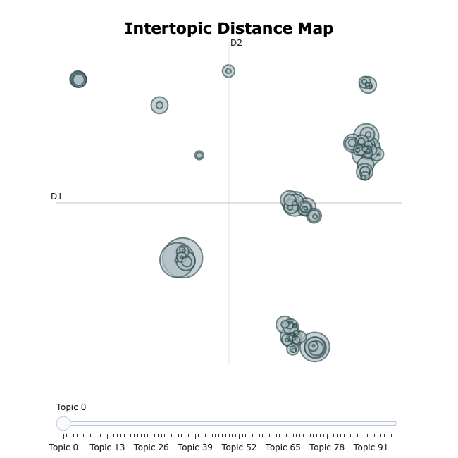
This command visualizes the hierarchical relations between topics:
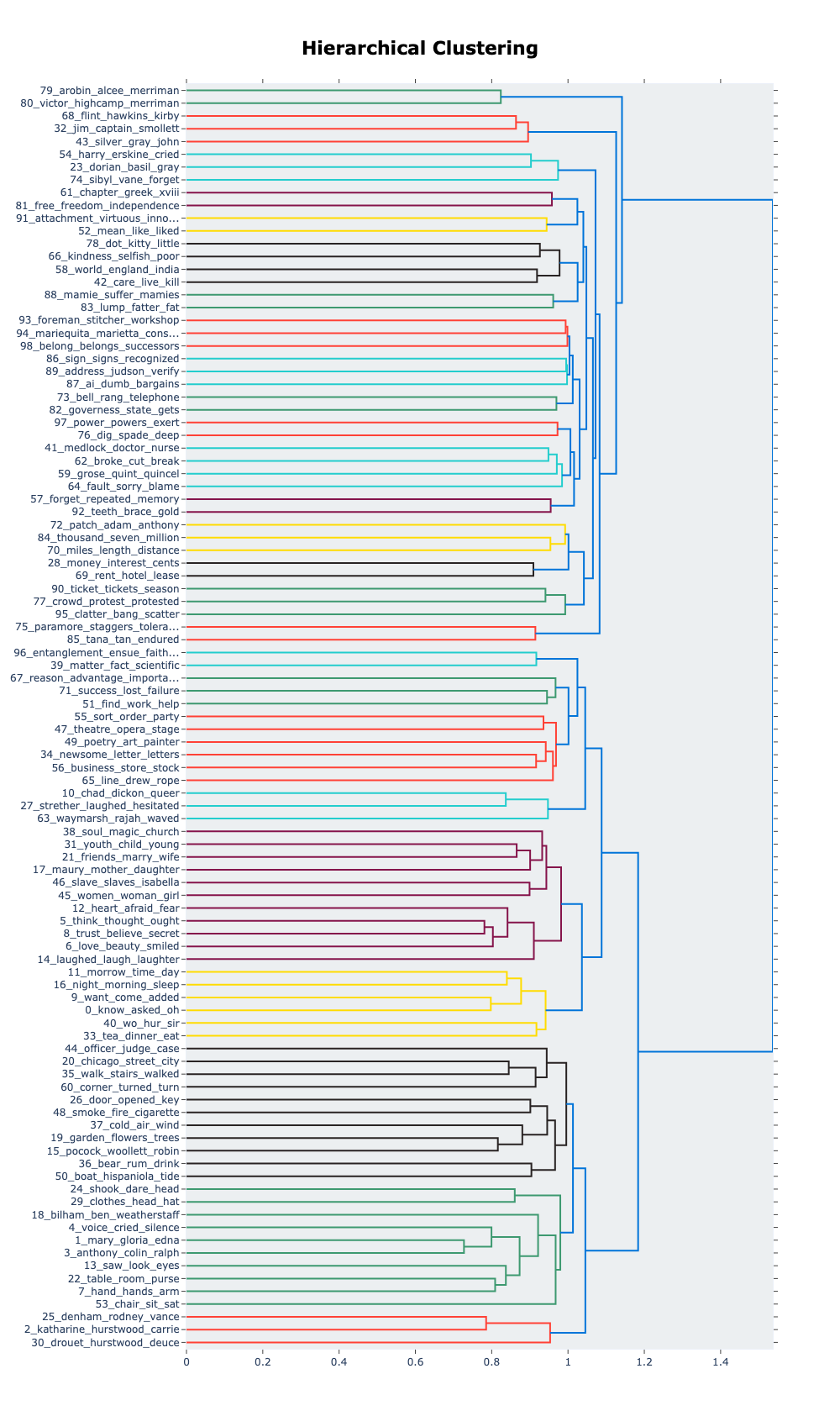
To find topics that are associated to a particular term, use the
.find_topics() method:
Visualize the terms of the topics found:
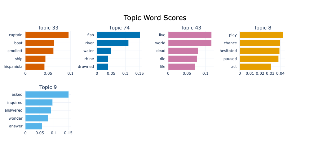
During the model training, all texts in the data have been assigned to a topic distribution. You can also use the model to infer the topics of previously unseen texts based on the same model:
OUTPUT
[20] [1.]This example was assigned to topic 20, with a score of 1.0. Again,
these numbers can vary per run. For less trivial sentences, the model
can assign multiple topics to a text. In that case, the
topics and probs lists contain the according
number of values.
Explore Topics and Modelling Parameters
- Pick three topics and assign a concise, descriptive label to it
- Change the number and minimum size of topics
(
BERTopic(nr_topics=..., min_topic_size=...)) and observe how topics change - Think of a way to evaluate the topic model systematically.
There is no general ‘true’ label for a topic, but looking at the top word of a topic should give an idea of the concept(s) it refers to, for instance:
[helen, gloria, miss, mary, edna, jane, martha, ...-> ‘female names and titles’[hurstwood, drouet, rochester, boldwood, ...-> ‘family names’[heart, exclaimed, shook, cried, tears, laugh, ...-> ‘emotions’
- Omitting the number of topics (
nr_topics) results in an ‘optimal’ number, according to the clustering algorithm. - Limiting the number of topics forces the algorithm to merge similar topics.
- Minimum topic sizes prevents the algorithm to form clusters of very few documents.
- Evaluation methods:
- Quantitative, extrinsic: apply model for downstream task, e.g. document classification, which can be evaluated empirically
- Quantitative, intrinsic, e.g.: measure overlap by words or documents, distance between topics
- Qualitative: define a research question; (how well) do the topics help you to approach it?
Step by Step
Under the hood, topic modelling means to create vector representations of topics. Topics are (even) harder to define than words because topics are not visible on the surface of a text – they are latent.
BERTopic provides reasonable defaults that typically provide a starting point that may work fine in many situations. The individual components of BERTopic can be adapted, each of which has impact on the final results. For that purpose, a deeper understanding of their inner workings allows you to adapt them to specific datasets or research questions.
1. Document Embeddings
In the first step, we need a vector representation of each document
that reflects their content. BERTopic makes use of existing models for
that purpose so that the specifics depend on the chosen model. By
default, it uses a Sentence
Transformers model called all-MiniLM-L6-v2,
a model that has been trained to generate semantic representations for
English texts with a maximum length of 256 word pieces; with a word
comprising one or multiple pieces. This model outputs vectors with 384
dimensions that represent an entire text sequence, like a sentence. The
distance between document-vectors in the vector space reflect the
semantic similarity of the respective texts.
Alternative Sentence Transformer models that are available on the HuggingFace platform can be used
through the embedding_model parameter in the
BERTopic object initialization. BERTopic can also use
models provided by other popular NLP frameworks, including spaCy and
Gensim. Additionally, you can provide pre-computed embeddings per
document.
By choosing a different language model you can adapt the BERTopic pipeline when other languages than English, longer texts, faster processing, higher accuracy, or different modelling algorithms are needed.
For corpora in which multiple languages occur, or languages for which
no specific model is available, the
paraphrase-multilingual-MiniLM-L12-v2 model is recommended.
It is loaded automatically, if language='multilingual' is
passed to the BERTopic object:
Any other model available on the HuggingFace platform can be loaded
via embedding_model – overriding the language
argument:
The same parameter is used for models from other platforms too, but those models need to be initialized separately and passed as objects like this:
2. Reduce dimensionality
The document embeddings computed in the previous step are quite large. To make the subsequent computations less costly regarding time and resources, the UMAP algorithm is applied to project vectors to a lower dimensionality while preserving their approximate mutual distance – this is the crucial property used in the next following steps. For instance, the 384-dimensional vectors generated by in the first step will be represented with five dimensions per documents.
Again, BERTopic offers using alternative algorithms like PCA (Principal Component Analysis), but UMAP provides the state-of-the-art algorithm for this specific task. Furthermore, this step could be skipped entirely; however, that will require much more time and resources in the following steps.
By default, the UMAP model for transforming the document embeddings
from step 1 to a lower dimensionality is computed on-the-fly. The
umap_model argument allows the specification of another
model that has been pre-computed:
In principle, any object can be passed here, as long as it has a
.transform(X) method that takes a vector X as
input, and outputs a vector.
3. Clustering
Based on the representations computed in the previous steps, the documents are grouped into clusters by mutual distance – hence the importance of preserving that property when reducing the dimensionality in step 2.
By default, BERTopic uses HDBScan (Hierarchical Density-Based Spatial Clustering of Applications with Noise).
This option is customisable, too; any clustering algorithm provided
by scikit-learn
can be used. Initialize the respective object according to its
specifics, and pass it to the hdbscan_model parameter:
PYTHON
from bertopic import BERTopic
from sklearn.cluster import KMeans

cluster_model = KMeans(n_clusters=50)
topic_model = BERTopic(hdbscan_model=cluster_model)
Again, however, the default is the best algorithm in most cases.
4. Topic Representation
Finally, a strong feat of topic modelling is that it extracts topics
that are interpretable by humans, as opposed to numeric representations.
This goal has been approached by displaying a list of the most
representative per topic by most topic modelling algorithms, including
BERTopic. For each topic, it calculates the most representative words
through a class-based adaption of the TF-IDF algorithm, called
c-TD-IDF.
TF-IDF means
Term Frequency - Inverse Document Frequency, a metric that
has been used for decades. In search and information retrieval
applications, TF-IDF estimates the relevancy of a term for a specific
document in the context of a document collection, based on two
factors:
- How frequently does the term occur in the document at hand? The more frequent a word, the higher its TF-IDF score for the document.
- In how many other documents in the collection does the term occur? The more documents contain a word, the lower its TF-IDF score.
The c-TF-IDF adaptation interprets each topic cluster as a class. For the score calculation, it views them as a single document and computes the cluster-specific TF-IDF values with the same factors as before:
- If a term occurs frequently in the documents of a topic, it gets a higher score.
- If a term occurs in many topics, it gets a lower score.
As a results, words that only occur in a single topic cluster are
considered to be most representative for that topic. Neverthless, it
allows for the inherent ambiguity of words as they can be relevant for
different topics. The word bank, for instance, could have a
high weight in a money-related topic as well as in a river-related topic
if it occurs frequently enough in those clusters, but rarely in
others.
At the same time, words that occur universally get a low score for
all clusters for not being topic-specific. Nevertheless, the calculation
can suffer under extreme frequencies of words like the and
a in English. Therefore, BERTopic removes such stop words
by default through a pre-defined list of English stop words.
In our case, however, no action is needed here because stop words have already been removed when the data was preprocessed above.
Model Tuning
BERTopic provides numerous parameters to tune its behaviour during
all the previously mentioned steps. The most important of them are
directly accessible through arguments when the BERTopic
object is initialized.
- Choose a different language model with
embedding_model; see the Document Embeddings section above and the HuggingFace model hub for suitable models that can be filtered by language, model size and other parameters. - Control the clustering parameters with
-
nr_topics: split topic clusters until it reaches exactly the specified number, or useautoto use the HDBSCAN algorithm to guess the optimal number of topic clusters. -
min_cluster_sizeormin_topic_size: A topic cluster must contain at least the given number of document; otherwise, it is merged with an adjacent cluster. This prevents the formation of topics based on very few data points. The default is5.
-
- An NLP pipeline is a chain of steps from raw text to a structured task output.
- Word embeddings represent words as dense numeric vectors. These are learned by training neural network(s) on a language modeling objective. Because similar words appear in similar contexts, semantically related words will have gemoetrically similar vectors.
- Word2Vec is a popular word embedding model. It encodes semantic relationships in vector arithmetic: analogies like “king − man + woman ≈ queen” emerge naturally from the geometry of vectors.
- Word2Vec has a key limitation: words unseen during training (out-of-vocabulary) cannot be represented, and each word receives one fixed vector regardless of context.
- Cosine similarity measures the angle between two vectors and is the standard metric for comparing word embeddings: it captures semantic relatedness independently of vector magnitude, and returns values between -1 (not similar at all) and 1 (completely similar).
- Topic modelling is an unsupervised method for discovering latent themes in a document collection, representing each topic as a weighted list of characteristic words and each document as a mixture of topics.
- BERTopic builds on language model embeddings by chaining document vectorization (each document gets a single vector that represents it), dimensionality reduction (UMAP), clustering (HDBSCAN), and topic labeling (c-TF-IDF) — each component can be swapped to adapt to different languages, text lengths, or research goals.
Content from Transformers: BERT and Beyond
Last updated on 2026-05-20 | Edit this page
Estimated time: 120 minutes
Overview
Questions
- What are some drawbacks of static word embeddings?
- What are Transformers?
- What is BERT and how does it work?
- How can I use BERT to solve supervised NLP tasks?
- How should I evaluate my classifiers?
Objectives
- Explain why contextualized vectors are an improvement
- Describe the Transformer architecture and its main components
- Explain what the BERT language model is
- Use the HuggingFace pipeline to run examples using BERT
- Use a pre-trained BERT model for text classification
- Apply basic evaluation metrics to assess the quality of any NLP model
Word embeddings such as Word2Vec can be used to represent words as unique vectors instead of Python strings. These vector representations give us numerical “proxy” representations for words. And these allow us to provide mathematical definitions for attributing semantics or meaning to words. They also enable metrics and measures for studying linguistic relationships with words. For example, one can devise metrics for similarity and semantic closeness of words, by defining a measure of distance between their corresponding vectors. This has proven to be quite useful for downstream lexical-related tasks.
However, a big drawback of Word2Vec is that each word is represented in isolation, which means that once we finished training a model, each word has exactly one vector associated with it, regardless of the different contexts in which it appears in the corpus text. This is what is called static word embedding, and unfortunately that is a serious limitation in expressing finer-grained complexities in language. Words derive their meaning dynamically, based on the specific context in which they are used. Think of syntactic information, which is relevant to understand the difference between “the dog bit the man” and “the man bit the dog”. Another case is polysemy, where the same word can have very different meanings depending on the context, for example, “bit” in “the dog bit the man” and “in this bit of the book”. Therefore, we would like to have richer vectors of words that are themselves sensitive to their context in order to obtain finer-grained representations of word meaning.
Polysemy in Language
Think of words (at least 2) that can have more than one meaning depending on the context. Come up with one simple sentence per meaning and explain what they mean in each context. Discuss: How do you know which of the possible meanings does the word have when you see it?
Two possible examples can be the words ‘fine’ and ‘run’
Sentences for ‘fine’: - She has a fine watch (fine == high-quality) - He had to pay a fine (fine == penalty) - I am feeling fine (fine == not bad)
Sentences for ‘run’: - I had to run to catch the bus (run == moving fast) - Stop talking, before you run out of ideas (run (out) == exhaust)
Note how in the “run out” example we even have to understand that the meaning of run is not literal but goes accompanied with a preposition that changes its meaning.
Bridging Word Embeddings and Contextualized Models
The limitations of Word2Vec became apparent as researchers tackled more complex natural language understanding tasks. BERT, the model we will describe below, was not the first attempt to improve upon the drawbacks of Word2Vec. Several intermediate models emerged to address the shortcomings. Some prominent models were:
FastText (Joulin, et. al., 2016), developed by Facebook, extended Word2Vec by representing words as bags of character n-grams rather than atomic units. This subword tokenization approach enabled the model to generate embeddings for previously unseen words by combining learned subword representations—for instance, understanding “unhappiness” through its components “un-,” “happiness,” and “-ness.” FastText proved particularly valuable for morphologically rich languages and handling misspellings or rare word forms.
ELMo (Peters, et. al., 2018) marked a paradigm shift by integrating context into the word representations. Unlike Word2Vec’s static embeddings, ELMo generated different representations for the same word based on its surrounding context using bidirectional LSTM networks. The model was pretrained on large text corpora using a language modeling objective—predicting words from both left and right contexts simultaneously—and crucially introduced effective transfer learning to NLP. BERT would basically replicate this concept but using a more powerful neural network architecture: the Transformer, which allowed for the scaling of training material.
ULMFiT (Howard & Ruder, 2018). Universal Language Model Fine-tuning, also tackled the problem via transfer learning; that is, re-using the same model for learning several different tasks and hence enriching word representations after each task was learned. This idea also enriched BERT post-training methodologies.
These intermediate models established several crucial concepts: that subword tokenization could handle vocabulary limitations, that context-dependent representations were superior to static embeddings, that deep bidirectional architectures captured richer linguistic information, and most importantly, that large-scale pretraining followed by task-specific fine-tuning could dramatically improve performance across diverse NLP applications.
In late 2018, the BERT language model was introduced. Using a novel architecture called Transformer (2017), BERT was specifically designed to scale the amount of training data and integrate context into word representations. To understand BERT, we will first look at what a transformer is and we will then directly use some code to make use of BERT.
Transformers
The Transformer is a deep neural network architecture proposed by Google researchers in a paper called Attention is all you Need. They tackled specifically the NLP task of Machine Translation (MT), which is stated as: how to generate a sentence (sequence of words) in target language B given a sentence in source language A? We all know that translation cannot be done word by word in isolation, therefore integrating the context from both the source language and the target language is necessary. In order to translate, first one neural network needs to encode the whole meaning of the sentence in language A into a single vector representation, then a second neural network needs to decode that representation into tokens that are both coherent with the meaning of language A and understandable in language B. Therefore we say that translation is modeling language B conditioned on what language A originally said.
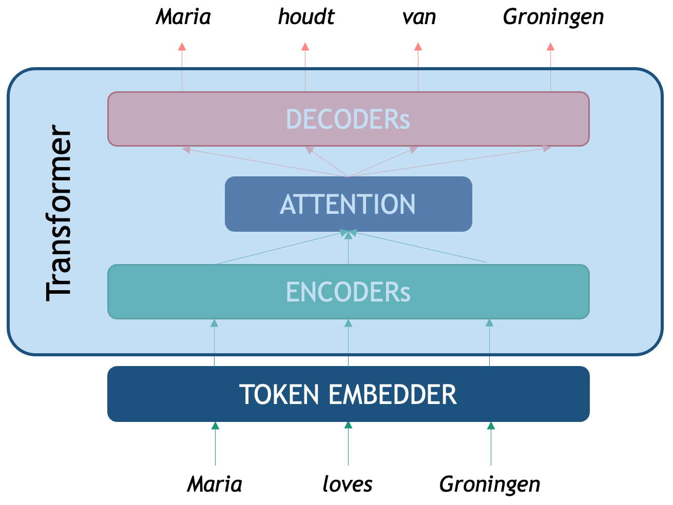
As seen in the picture, the original Transformer is an Encoder-Decoder network that tackles translation. We first need a token embedder which converts the string of words into a sequence of vectors that the Transformer network can process. The first component, the Encoder, is optimized for creating rich representations of the source sequence (in this case an English sentence) while the second one, the Decoder is a generative network that is conditioned on the encoded representation. The third component we see is the infamous attention mechanism, a third neural network what computes the correlation between source and target tokens (which word in Dutch should I pay attention to, to decide a better next English word?) to generate the most likely token in the target sequence (in this case Dutch words).
Emulate the Attention Mechanism
Pair with a person who speaks a language different from English (we will call it language B). Think of 1 or 2 simple sentences in English and come up with their translations in the second language. In a piece of paper write down both sentences (one on top of the other with some distance in between) and try to:
- Draw a mapping of words or phrases from language B to English. Is it always possible to do this one-to-one for words?
- Think of how this might relate to attention in transformers?
Here is an example of a sentence in English and its translation into Spanish. We can look at the final mapping and observe that:
- Even though they are closely related languages, the translation is not linear
- There is also not a direct word-to-word mapping between the sentences
- Some words present in the source are not present in the target (and vice versa)
- Some words are not translations of each other but they are still very relevant to understand the context
Next, we will see how BERT exploits the idea of a Transformer Encoder to perform the NLP Task we are interested in: generating powerful word representations.
BERT
BERT is an acronym that stands for Bidirectional Encoder Representations from Transformers. The name describes it all: the idea is to use the power of the Encoder component of the Transformer architecture to create powerful token representations that preserve the contextual meaning of the whole input segment, instead of each word in isolation. The BERT vector representations of each token take into account both the left context (what comes before the word) and the right context (what comes after the word). Another advantage of the transformer Encoder is that it is parallelizable, which made it possible for the first time to train these networks on millions of datapoints, dramatically improving model generalization.
Pretraining BERT
The notion of ‘pre-trained’ describes a model that has already been optimised on relevant data for a given task. Such a model can typically be loaded and applied directly to new datasets, often working “out of the box” without the need for further refinement. Ideally, publicly released pre-trained models have undergone rigorous testing for both generalisation and output quality on different textual data that it was intended to be used on. Nevertheless, it remains essential to carefully review the evaluation methods before relying on them in practice. It is also recommended that you perform your own evaluation of the model on text that you intend to use it on.
A pre-trained model can be of good quality for some data, but might not fit the nuances of our specific dataset. For example, the model was trained on newspaper articles but you are interested in poetry. In this case, it is common to perform fine-tuning: instead of training your own model from scratch, you start with the knowledge obtained in the pre-trained model and adjust (fine-tune) it to your specific data to increase its performance on the specific task you are trying to solve. The advantage of fine-tuning is that you often do not need a large amount of data to improve the results, hence the popularity of the technique.
BERT models have been pre-trained with the goal of obtaining vector representation through two tasks:
Masked Language Model: for each sentence, mask one token at a time and predict which token is missing based on the context from both sides. A training input example would be “Maria [MASK] Groningen” and the model should predict the word “loves”.
Next Sentence Prediction: the Encoder gets a linear binary classifier on top, which is trained to decide if sequence A precedes sequence B in a text, for each pair of sequences A and B. For the sentence pair: “Maria loves Groningen.” and “This is a city in the Netherlands.” the output of the classifier is “True” and for the pair “Maria loves Groningen.” and “It was a tasty cake.” the output should be “false” as there is no obvious continuation between the two sentences.
Already the second pre-training task gives us an idea of the power of BERT: after it has been trained on hundreds of thousands of texts, one can add a classifier on top and re-use the linguistic knowledge previously acquired to fine-tune it for a specific task, without needing to learn the weights of the whole network from scratch all over again.
This model and hundreds of related transformer-based pre-trained encoders can also be found on Hugging Face.
BERT Architecture
The BERT Architecture can be seen as a basic NLP pipeline on its own:
- Tokenizer: splits text into tokens that the model recognizes
- Embedder: converts each token into a fixed-sized vector that represents it. These vectors are the actual input for the Encoder.
- Encoder several neural layers that model the token-level interactions of the input sequence to enhance meaning representation. The output of the encoder is a set of Hidden layers, the vector representation of the ingested sequence.
- Output Layer: the final encoder layer (which we depict as a sequence H’s in the figure) contains arguably the best token-level representations that encode syntactic and semantic properties of each token, but this time each vector is already contextualized with the specific sequence.
- OPTIONAL Classifier Layer: an additional classifier can be connected on top of the BERT token vectors which are used as features for performing a downstream task. This can be used to classify at the text level, for example sentiment analysis of a sentence, or at the token-level, for example Named Entity Recognition.
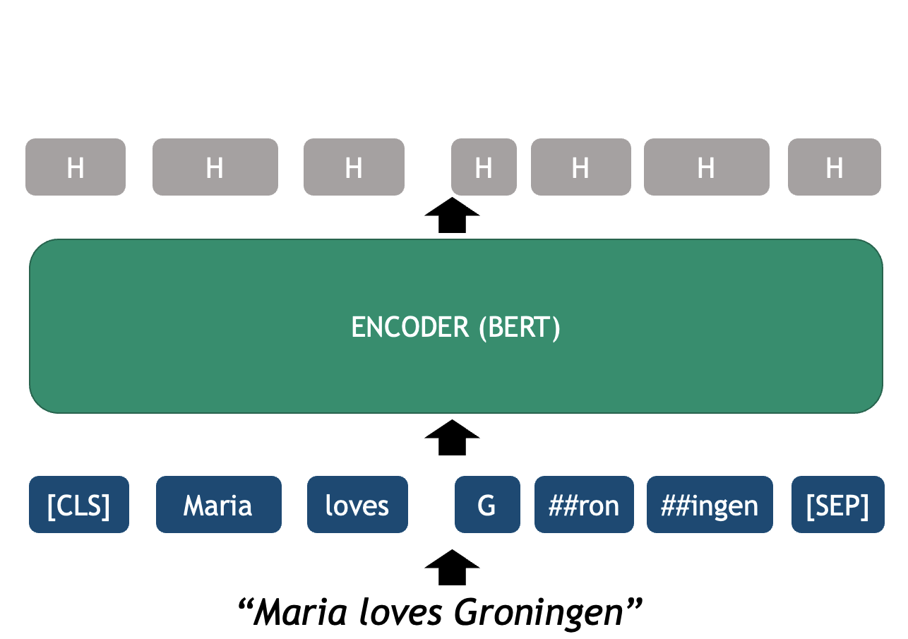
BERT uses (self-) attention, which is very useful to capture longer-range word dependencies such as co-reference, where, for example, a pronoun can be linked to the noun it refers to previously in the same sentence. See the following example:
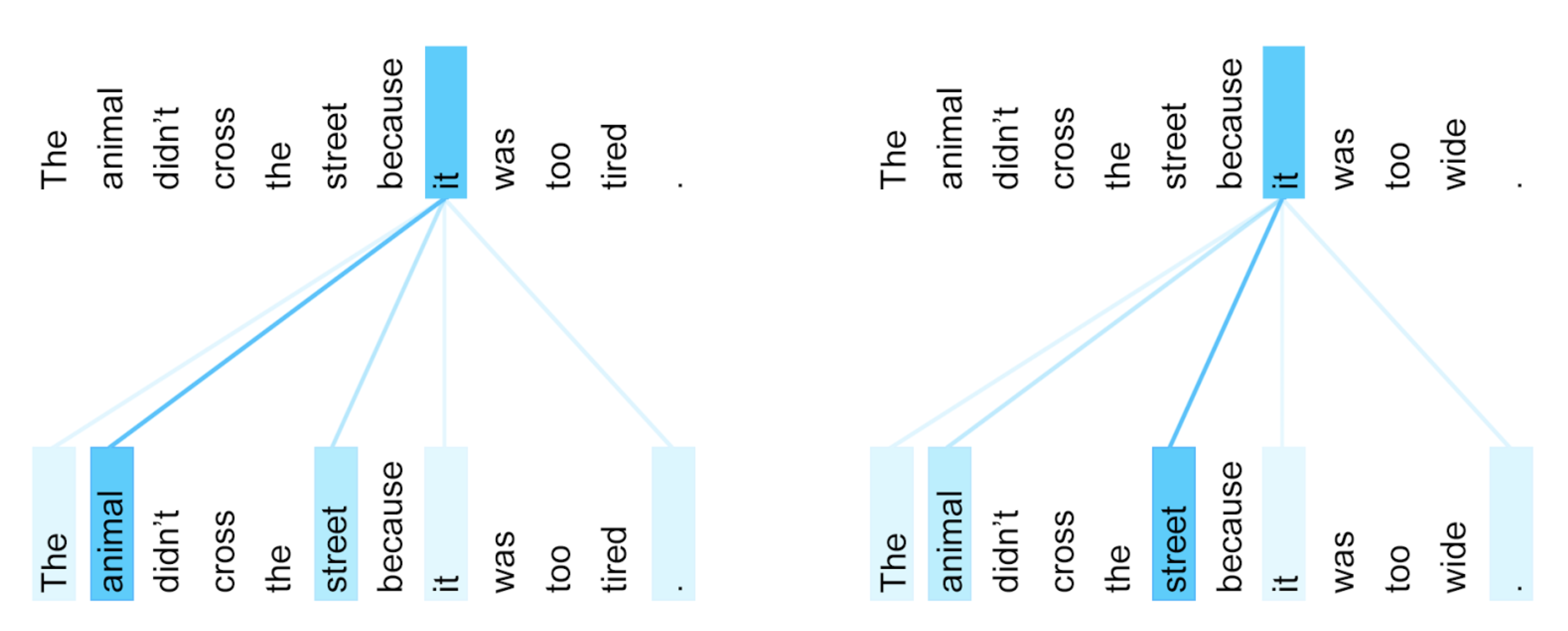
BERT for Word-Based Analysis
Let’s see how these components can be manipulated with code. For this we will be using the HuggingFace’s transformers Python library. The first two main components we need to initialize are the model and tokenizer. The HuggingFace hub contains thousands of models based on a Transformer architecture for dozens of tasks, data domains and also hundreds of languages. Here we will explore the vanilla English BERT which was how everything started. We can initialize this model with the next lines:
PYTHON
from transformers import BertTokenizer, BertModel
tokenizer = BertTokenizer.from_pretrained('bert-base-cased')
model = BertModel.from_pretrained("bert-base-cased")
BERT Tokenizer
We start with a string of text as written in any blog, book,
newspaper etcetera. The tokenizer object is responsible of
splitting the string into recognizable tokens for the model and
embedding the tokens into their vector representations
PYTHON
text = "Maria loves Groningen"
encoded_input = tokenizer(text, return_tensors='pt')
print(encoded_input)
The print shows the encoded_input object returned by the
tokenizer, with its attributes and values. The input_ids
are the most important output for now, as these are the token IDs
recognized by BERT
{
    'input_ids': tensor([[  101,  3406,  7871,   144,  3484, 15016,   102]]),
    'token_type_ids': tensor([[0, 0, 0, 0, 0, 0, 0]]),
    'attention_mask': tensor([[1, 1, 1, 1, 1, 1, 1]])
}
NOTE: the printing function shows transformers objects as dictionaries; however, to access the attributes, you must use the Python object syntax, such as in the following example:
Output:
torch.Size([1, 7])
The output is a 2-dimensional tensor where the first dimension contains 1 element (this dimension represents the batch size), and the second dimension contains 7 elements which are equivalent to the 7 tokens that BERT generated from our string input.
In order to see what these Token IDs represent, we can
translate them into human readable strings. This includes
converting the tensors into numpy arrays and converting
each ID into its string representation:
PYTHON
token_ids = list(encoded_input.input_ids[0].detach().numpy())
string_tokens = tokenizer.convert_ids_to_tokens(token_ids)
print("IDs:", token_ids)
print("TOKENS:", string_tokens)
IDs: [101, 3406, 7871, 144, 3484, 15016, 102]
TOKENS: ['[CLS]', 'Maria', 'loves', 'G', '##ron', '##ingen', '[SEP]']
First we feed the tokenized input into the model:
Now we can explore the representations in the model.
In the case of wanting to obtain a single vector for Groningen, you can average the three vectors that belong to the token pieces that ultimately form that word. For example:
PYTHON
import numpy as np
tok_G = output.last_hidden_state[0][3].detach().numpy()
tok_ron = output.last_hidden_state[0][4].detach().numpy()
tok_ingen = output.last_hidden_state[0][5].detach().numpy()

tok_groningen = np.mean([tok_G, tok_ron, tok_ingen], axis=0)
print(tok_groningen.shape)
print(tok_groningen[:10])
We obtain the output:
(768,)
[ 0.00990007 -0.44266668  0.05274092  0.08865168  0.71115637 -0.4092603
  0.18841815  0.19883917  0.24680579 -0.07899686]
We use the functions detach().numpy() to bring the
values from the Pytorch execution environment (for example a GPU) into
the main Python thread and treat it as a Numpy vector for
convenience. Then, since we are dealing with three Numpy
vectors we can average the three of them and end up with a single
Groningen vector of 768-dimensions representing the average
of 'G', '##ron', '##ingen'.
Analyzing polysemy with BERT
We can encode two sentences containing the word note to see how BERT actually handles polysemy (note means something very different in each sentence) thanks to the representation of each word now being contextualized instead of isolated as was the case with Word2vec.
PYTHON
# We tokenize the sentence and identify the two different 'note' tokens inside the sentence
text_note = "Please note that this bank note is fake!"
tokenized_text = tokenizer(text_note, return_tensors='pt')
token_ids = list(tokenized_text.input_ids[0].detach().numpy())
string_tokens = tokenizer.convert_ids_to_tokens(token_ids)
print(string_tokens)
We are printing the BERT tokens extracted from the sentence, and displaying them:
['[CLS]', 'Please', 'note', 'that', 'this', 'bank', 'note', 'is', 'fake', '!', '[SEP]']We then manually count which token indices in the list belong to
note, so we can extract their vectors later
PYTHON
note_index_1 = 2 # first occurrence of `note`
note_index_2 = 6 # second occurrence of `note`
print(string_tokens[note_index_1], string_tokens[note_index_2])
We now pass the sentence through the BERT encoder and extract the
encoded vectors belonging to each note token:
PYTHON
import torch
# Encode the sentence and extract the vector belonging to each 'note' token
with torch.no_grad():
    bert_output = model(**tokenized_text)
note_vector_1 = bert_output.last_hidden_state[0][note_index_1].detach().numpy()
note_vector_2 = bert_output.last_hidden_state[0][note_index_2].detach().numpy()

print(note_vector_1[:5])
print(note_vector_2[:5])
[1.0170387 0.93691176 0.30571502 0.33091038 0.73093796]
[0.17840035 0.65847856 0.22412607 0.21162085 0.5393072 ]By printing the first 5 dimensions of the vectors we can see that,
even though both vectors technically belong to the same string input
note, they have different numeric representations. This is
the case because the BERT encoder takes into account the position of the
token as well as all the previous and following tokens when computing
the representation for each token.
To be sure, we can compute the cosine similarity of the word
note in the first sentence and the word note in
the second sentence confirming that they are indeed two different
representations, even when both cases have the same token-id and they
are the 12th token of the sentence:
PYTHON
from sklearn.metrics.pairwise import cosine_similarity
import numpy as np

vector1 = np.array(note_vector_1).reshape(1, -1)  # Reshape to 2D array
vector2 = np.array(note_vector_2).reshape(1, -1)  # Reshape to 2D array

similarity = cosine_similarity(vector1, vector2)
print(f"Cosine Similarity 'note' vs 'note': {similarity[0][0]}")
With this small experiment, we have confirmed that the Encoder produces context-dependent word representations, as opposed to Word2Vec, where note would always have the same vector no matter where it appeared.
When running examples in a BERT pre-trained model, it is advisable to
wrap your code inside a torch.no_grad(): context. This is
linked to the fact that BERT is a Neural Network that has been trained
(and can be further fine-tuned) with the Backpropagation algorithm.
Essentially, this wrapper tells the model that we are not in training
mode, and we are not interested in updating the weights (as it
would happen when training any neural network), because the weights are
already optimal enough. By using this wrapper, we make the model more
efficient as it does not need to calculate the gradients for an eventual
backpropagation step, since we are only interested in what comes
out of the Encoder. So the previous code can be made more efficient
like this:
BERT as a Language Model
As mentioned before, the main pre-training task of BERT is Language
Modelling (LM): calculating the probability of a word based on the known
neighboring words (yes, Word2Vec was also a kind of LM!). Obtaining
training data for this task is very cheap, as all we need is millions of
sentences from existing texts, without any labels. In this setting, BERT
encodes a sequence of words, and predicts from a set of English tokens,
what is the most likely token that could be inserted in the
[MASK] position
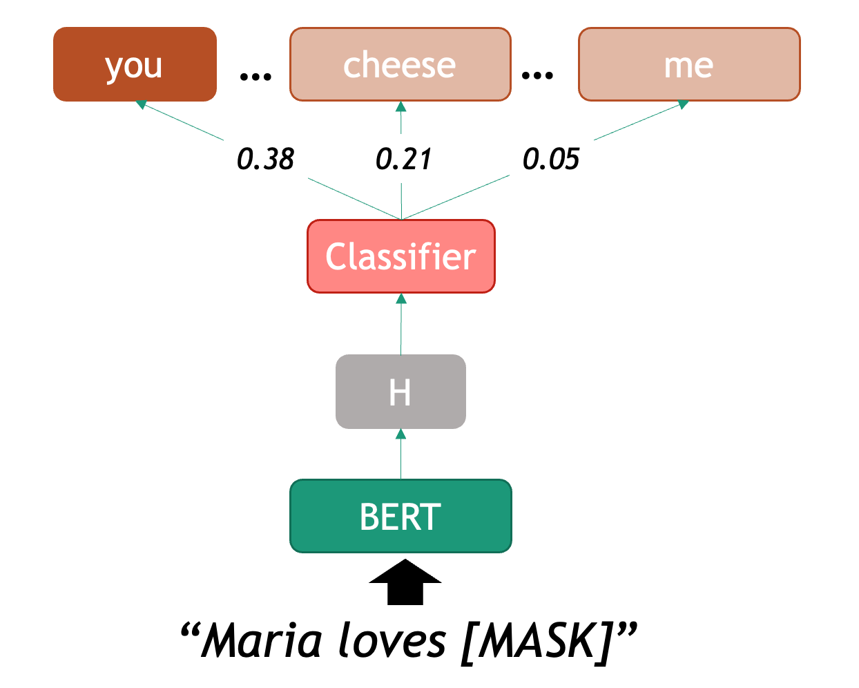
We can therefore start using BERT as a predictor for word completion.
From now own, we will learn how to use the pipeline object,
this is very useful when we only want to use a pre-trained model for
predictions (no need to fine-tune or do word-specific analysis). The
pipeline will internally initialize both model and
tokenizer for us and also merge word pieces back into complete
words.
The pipeline object is very convenient to test all the
out-of-the-box models that you can find in the HuggingFace platform, and
if you are lucky and you like what you see, this is the fastest way to
get model predictions.
But consider that for some tasks you will want more control over the tokenization and how the model merges the predictions. If that is the case, initializing the tokenizer, encoding the texts into word-vectors and running the model inference yourself might be the way to go (like it is shown in the Polysemy in BERT section).
Even if you like what you see, it is important that you evaluate the performance of the models in your data and use case regardless of what the model performance claims to be. We will show an example with a couple of evaluation metrics in the BERT for Text Classification section.
In this case again we use bert-base-cased, which refers
to the vanilla BERT English model. Once we declared a pipeline, we can
feed it with sentences that contain one masked token at a time (beware
that BERT can only predict one word at a time, since that was its
training scheme). For example:
PYTHON
from transformers import pipeline

def pretty_print_outputs(sentences, model_outputs):
    for i, model_out in enumerate(model_outputs):
        print("\n=====\t",sentences[i])
        for label_scores in model_out:
            print(label_scores)


nlp = pipeline(task="fill-mask", model="bert-base-cased", tokenizer="bert-base-cased")
sentences = ["Paris is the [MASK] of France", "I want to eat a cold [MASK] this afternoon", "Maria [MASK] Groningen"]
model_outputs = nlp(sentences, top_k=5)
pretty_print_outputs(sentences, model_outputs)
===== Paris is the [MASK] of France
{'score': 0.9807965755462646, 'token': 2364, 'token_str': 'capital', 'sequence': 'Paris is the capital of France'}
{'score': 0.004513159394264221, 'token': 6299, 'token_str': 'Capital', 'sequence': 'Paris is the Capital of France'}
{'score': 0.004281804896891117, 'token': 2057, 'token_str': 'center', 'sequence': 'Paris is the center of France'}
{'score': 0.002848200500011444, 'token': 2642, 'token_str': 'centre', 'sequence': 'Paris is the centre of France'}
{'score': 0.0022805952467024326, 'token': 1331, 'token_str': 'city', 'sequence': 'Paris is the city of France'}
===== I want to eat a cold [MASK] this afternoon
{'score': 0.19168031215667725, 'token': 13473, 'token_str': 'pizza', 'sequence': 'I want to eat a cold pizza this afternoon'}
{'score': 0.14800849556922913, 'token': 25138, 'token_str': 'turkey', 'sequence': 'I want to eat a cold turkey this afternoon'}
{'score': 0.14620967209339142, 'token': 14327, 'token_str': 'sandwich', 'sequence': 'I want to eat a cold sandwich this afternoon'}
{'score': 0.09997560828924179, 'token': 5953, 'token_str': 'lunch', 'sequence': 'I want to eat a cold lunch this afternoon'}
{'score': 0.06001955270767212, 'token': 4014, 'token_str': 'dinner', 'sequence': 'I want to eat a cold dinner this afternoon'}
===== Maria [MASK] Groningen
{'score': 0.24399833381175995, 'token': 117, 'token_str': ',', 'sequence': 'Maria, Groningen'}
{'score': 0.12300779670476913, 'token': 1104, 'token_str': 'of', 'sequence': 'Maria of Groningen'}
{'score': 0.11991506069898605, 'token': 1107, 'token_str': 'in', 'sequence': 'Maria in Groningen'}
{'score': 0.07722211629152298, 'token': 1306, 'token_str': '##m', 'sequence': 'Mariam Groningen'}
{'score': 0.0632941722869873, 'token': 118, 'token_str': '-', 'sequence': 'Maria - Groningen'}
When we call the nlp pipeline, requesting to return the
top_k most likely suggestions to complete the provided
sentences (in this case k=5). The pipeline returns a list
of outputs as Python dictionaries. Depending on the task, the fields of
the dictionary will differ. In this case, the fill-mask
task returns a score (between 0 and 1, the higher the score the more
likely the token is), a tokenId, and its corresponding string, as well
as the full “unmasked” sequence.
In the list of outputs we can observe: the first example shows correctly that the missing token in the first sentence is capital, the second example is a bit more ambiguous, but the model at least uses the context to correctly predict a series of items that can be eaten (unfortunately, none of its suggestions sound very tasty); finally, the third example gives almost no useful context so the model plays it safe and only suggests prepositions or punctuation. This already shows some of the weaknesses of the approach.
Challenge
Play with the fill-mask pipeline and try to find
examples where the model gives bad predictions and examples where the
predictions are very good. You can try:
- Changing the
top_kparameter - Test the multilingual BERT model to compare. To do this, you should
change the
modelandtokenizerparameter name tobert-base-multilingual-cased - Search for bias in completions. For example, compare predictions for “This man works as a [MASK].” vs. “This woman works as a [MASK].”.
This is a free exercise, so anything works. But even by running the same cases with the multilingual models we see some interesting aspects. For example, the predictions are of less quality in English. This is due to the “spread” of information across other languages, including a worse tokenization, since this model tries do predict for around 200 languages.
Another interesting example is searching for bias in the
completions, these can be bias in many areas. In this case,
comparing the outputs you get for the sentences “This man works as a
[MASK].” and “This woman works as a [MASK].” exposes the huge gender
biases inside BERT word representations: for ‘man’ BERT predicts
['lawyer', 'carpenter', 'doctor', 'waiter', 'mechanic'] and
for woman it predicts
['nurse', 'waitress', 'teacher', 'main', 'prostitute'].
We will next see the case of combining BERT with a classifier on top.
BERT for Text Classification
The task of text classification is assigning a label to a whole
sequence of tokens, for example a sentence. With the parameter
task="text_classification" the pipeline()
function will load the base model and automatically add a task-specific
layer.
The labels or categories depend on the task the model has been
trained for, hence the data. There are binary
classification tasks, e.g. spam or no spam, or
multiclass tasks, e.g. various emotions such as
anger, love, confusion etc.
Depending on the task, a model can assign exactly one label to each instance, or multiple. The latter is called a multi-label classification task.
Example: Emotion Classification
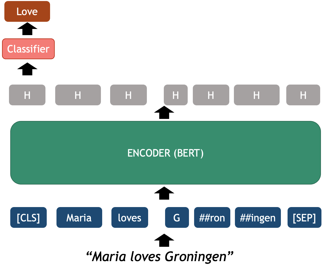
Let’s see the example of a emotion classifier based on
RoBERTa model. The roberta-base-go_emotions
model was trained on the GoEmotions
dataset, taken from English Reddit and labelled for 28 different
emotions at the sentence level. This model takes a sentence as input and
outputs a score for each of the 28 possible emotions that might be
conveyed in the text. For example:
PYTHON
classifier = pipeline(task="text-classification", model="SamLowe/roberta-base-go_emotions", top_k=3)

sentences = ["I am not having a great day.", "This is a lovely and innocent sentence.", "Maria loves Groningen."]
model_outputs = classifier(sentences)

pretty_print_outputs(sentences, model_outputs)

=====	 I am not having a great day.
{'label': 'disappointment', 'score': 0.5044488906860352}
{'label': 'sadness', 'score': 0.3469431400299072}
{'label': 'annoyance', 'score': 0.08485794812440872}

=====	 This is a lovely and innocent sentence.
{'label': 'admiration', 'score': 0.7667419910430908}
{'label': 'approval', 'score': 0.4139412045478821}
{'label': 'love', 'score': 0.1130351722240448}

=====	 Maria loves Groningen.
{'label': 'love', 'score': 0.9160982370376587}
{'label': 'neutral', 'score': 0.07024713605642319}
{'label': 'approval', 'score': 0.02595525234937668}
For each sentence, this code outputs a list with the
top-k (k=3) emotions to which the model has
assigned the highest scores. Because it is trained on a multi-label
dataset, multiple labels can have a high score.
In the process of fine-tuning, a generic language model like BERT is adapted to a specific task like text classification. This is faster than training a whole model, because we only need to train the classifier layer, a small neural network, that can learn to choose between the classes (labels) for your custom classification problem. This classifier is a single-layer neural network that assigns scores over a set of labels. It uses the input features provided by BERT, which already encodes the meaning of the entire sequence in its hidden states. You can learn more about fine-tuning BERT-like models in this HuggingFace tutorial.
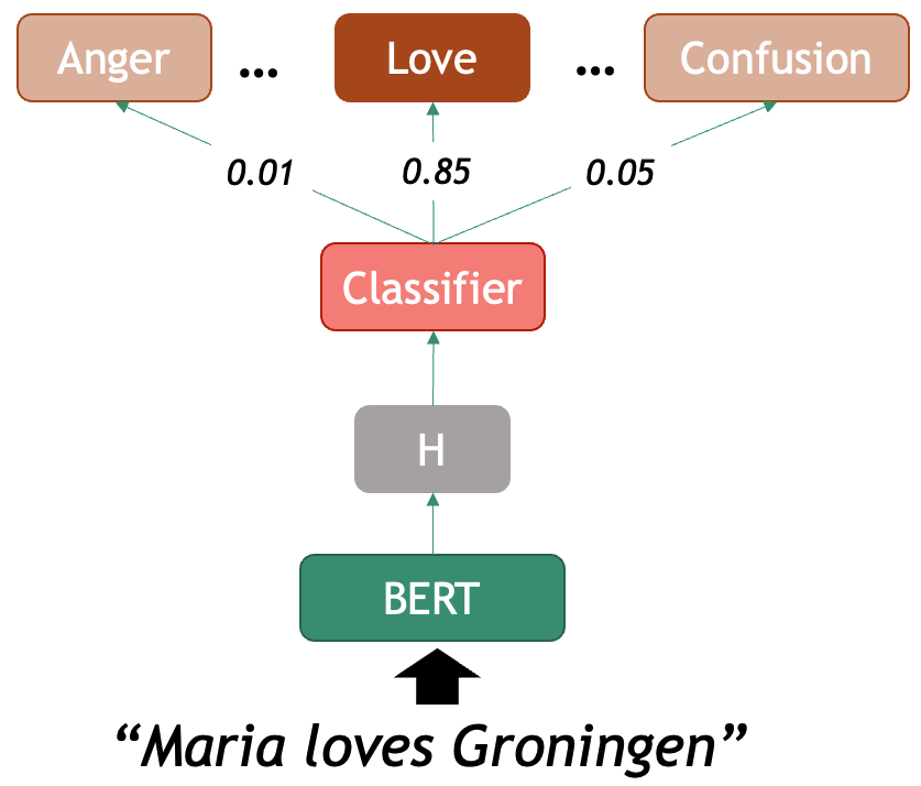
Model Evaluation
Model evaluation is a critical step in any machine learning project, and it is also the case for NLP. While it may be tempting to rely on the accuracy scores observed during training, or the model descriptions provided on the web, this approach can be misleading and often results in models that fail in real-world applications, and that includes your data.
The fundamental principle of model evaluation is to test your model on data it has never seen before. If you are training your own models, this is typically achieved by splitting your dataset into training, validation, and test sets. The training set is used to teach the model, the validation set helps tune hyperparameters or other aspects of model development, and the test set provides a less biased assessment of the final model’s performance. Without this separation, you risk overfitting, where your model memorizes the training data rather than learning generalizable patterns.
If you are using out-of-the-box models, evaluation is also mandatory, as you must be sure that the outputs you obtain behave in the manner that you would expect. In this case you only need to design the test set (with human annotators) and measure the performance. It doesn’t matter how broadly a model was tested, you must always confirm that it is suitable for your intended usage. It is also not enough to use semi-automated evaluation, designing human-labeled data will also provide insightful information for shaping your own task and judging the predictions you get.
Evaluation Metrics
Several metrics are commonly used to evaluate NLP models, each offering different insights into performance. Here we will describe the 4 most used in suervised learning classifiers
Let’s look at the toy example of classifying sentiments conveyed in
texts. In this task, there are three classes: positive,
neutral, and negative. We have a model that
return the label positive,neutral or
negative given an input text. If we want to evaluate how
good is our model at recognizing positives, there are 4
possibilities when comparing with the ground truth (your labelled
data):
-
True Positives (TP): the number of
positivetexts the model correctly labelled aspositive. -
True Negatives (TN): the number of
non-
positivetexts correctly labelled as something else. -
False Positives (FP): the number of
non-
positivetexts the model mistakenly labelled aspositive. -
False Negatives (FN): the number of
positivetexts mistakenly labelled as something else.
Based on this simple counts, we can derive four metrics that inform us at scale about the performance of our classifiers:
- Accuracy: measures the global proportion of correct predictions, regardless of the class they hold. This is al true cases (TP + TN) divided by all tested instances (TP+TN+FP+FN).
- Precision: This answers the following question: “Of all the predictions the model made for a particular class, how many were actually correct?”. This is TP divided by (TP+FP).
- Recall: This answers the following question: “Of all the actual instances of a class, how many did the model successfully identify?”. This is TP divided by (TP+FN).
- F1-score: provides a harmonic mean of precision and recall, offering a single metric that balances both concerns.
Deciding which metric is the most relevant to your case depends on your specific task, but having a view at all of the metrics is always insightful.
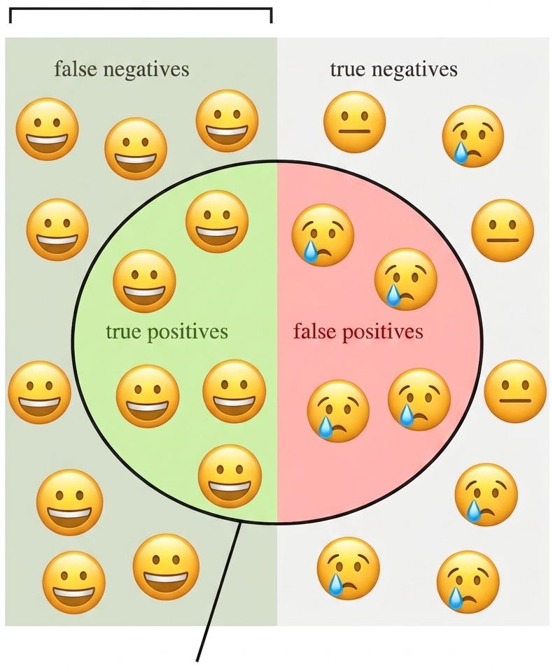
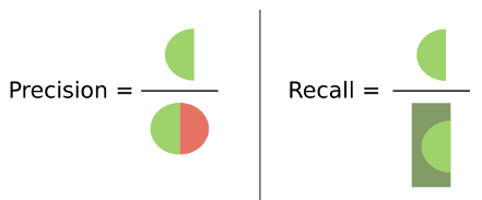
It’s important to remember that a high accuracy score doesn’t always indicate a good model. For example, if you’re classifying rare events that occur only 5% of the time, a naive model that always predicts “no event” would achieve 95% accuracy while being completely useless. This is why examining multiple metrics and understanding your data’s characteristics is essential for proper model evaluation.
In Python, the scikit-learn package already provides us
with these (and many other) evaluation metrics. All we need to do is
prepare an ordered list with the true_labels and a list
with the corresponding predicted_labels for each example in
our data.
Example: Sentiment Analysis
To illustrate the usage of evaluation, we will use a sentiment model
that predicts 5 classes: very positive,
positive, neutral, negative and
very negative. Here is an example of the model predictions
for four toy examples:
PYTHON
from transformers import pipeline

# Load the classification pipeline with the specified model
pipe = pipeline("text-classification", model="tabularisai/multilingual-sentiment-analysis")

# Classify a new sentence
sentences = [
    "I love this product! It's amazing and works perfectly.",
    "The movie was a bit boring, I could predict the ending since minute 1.",
    "Mary Shelley wrote this book around 1816.",
    "Everything suuuucks!"
]
gold_labels = [
    "Very Positive",
    "Negative",
    "Neutral",
    "Very Negative"
]

# The pipeline can also run on a batch of examples
result = pipe(sentences)

# Print the result
predicted_labels = []
for res in result:
    print(res)
    predicted_labels.append(res['label'])
{'label': 'Very Positive', 'score': 0.5586304068565369}
{'label': 'Negative', 'score': 0.9448591470718384}
{'label': 'Neutral', 'score': 0.9229359030723572}
{'label': 'Very Negative', 'score': 0.36225152015686035}We can see that the model predicts correctly the 4 examples we gave. This is unsurprising as they are incredibly obvious examples. We can also print the results and inspect them because they are only 4 instances, but it is clearly not a scalable approach.
Note that many models assign scores to their predictions. It is very tempting to interpret these scores as a proxy for “how certain is the model of prediction X”. However, this score is only a relative measure with respect to the training data, and it does not always translate well to unseen data.
We can obtain an automated evaluation report, including the basic
evaluation metrics, from scikit-learn by calling:
PYTHON
from sklearn.metrics import classification_report

print(classification_report(y_true=gold_labels, y_pred=predicted_labels))
The output is a table showing a breakdown of metrics by class. The
column support shows how many examples per class were
present in the gold data.
               precision    recall  f1-score   support

     Negative       1.00      1.00      1.00         1
      Neutral       1.00      1.00      1.00         1
Very Negative       1.00      1.00      1.00         1
Very Positive       1.00      1.00      1.00         1

     accuracy                           1.00         4
    macro avg       1.00      1.00      1.00         4
 weighted avg       1.00      1.00      1.00         4
These 4 metrics range from 0 to 1 (note that sometimes people multiply the scores by 100 to gain more granularity with decimal places). In this case, because we had a perfect score everything amounts to 1. In the most catastrophic scenario all scores would be zero.
Evaluate Sentiment Classifier
Now it is time to scale things a little bit more… Use the same
pipeline from the given toy example to run predictions over 100 examples
of short book reviews. Then print the classification report for the
given test set. These examples are given in the
data/sentiment_film_data.tsv file.
You can use the following helper functions, the first one helps you read the file and the second one normalizes the 5-class predictions into the 3-class annotations given in the test set:
PYTHON
def load_data(filename):
    with open(filename, 'r') as f:
        lines = f.readlines()[1:] # skip header
    sentences, labels = zip(*(line.strip().split('\t') for line in lines))
    return list(sentences), list(labels)

def get_normalized_labels(predictions):
    # predictions is a list with dicts such as {'label': 'positive', 'score': 0.95}
    # We also need to normalize the labels to match the true labels (which are only 'positive' and 'negative')
    normalized = []
    for pred in predictions:
        label = pred['label'].lower()
        if 'positive' in label:
            normalized.append('positive')
        elif 'negative' in label:
            normalized.append('negative')
        else:
            normalized.append('neutral')
return normalizedPYTHON
from sklearn.metrics import classification_report, precision_recall_fscore_support
import matplotlib.pyplot as plt

sentences, labels = load_data('data/sentiment_film_data.tsv')
# The labels from our dataset
y_true = labels
# Run the model to get predictions per sentence
y_pred = pipe(sentences)
# Normalize the labels to match the gold standard
y_pred = get_normalized_labels(y_pred)

# Detailed report with all metrics
print(classification_report(y_true, y_pred))
Here is the classification report:
OUTPUT
              precision    recall  f1-score   support

    negative       0.57      1.00      0.73        23
     neutral       0.53      0.22      0.31        37
    positive       0.69      0.78      0.73        40

    accuracy                           0.62       100
   macro avg       0.60      0.66      0.59       100
weighted avg       0.61      0.62      0.57       100
Confusion Matrix
The confusion matrix is another direct and informative tool for understanding your model’s performance, by offering an intuitive visualization of your model’s behavior in detail. It is a table that compares your model’s predictions against the true labels. The rows typically represent the actual classes, while the columns show the predicted classes. Each cell contains the count of instances that fall into that particular combination of true and predicted labels. Perfect predictions would result in all counts appearing along the diagonal of the matrix, with zeros everywhere else.
PYTHON
import matplotlib.pyplot as plt

from sklearn.metrics import ConfusionMatrixDisplay

def show_confusion_matrix(y_true, y_pred, labels=None):
    ConfusionMatrixDisplay.from_predictions(y_true, y_pred, display_labels=labels, cmap='Blues')
    plt.show()

show_confusion_matrix(y_true, y_pred)
This code shows the following matrix:
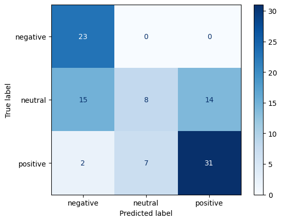
Some of the insights from a confusion matrix include:
- Observe which classes your model handles well and which ones it struggles with.
- Observe confusion patterns between classes. By examining the off-diagonal cells, you can identify systematic errors your model makes. For example, perhaps your sentiment classifier consistently confuses neutral statements with positive ones, but rarely mistakes neutral for negative.
- Detect Bias, for example by exposing a tendency to over-predict certain classes while ignoring others.
- Detect class imbalance. Even if your overall accuracy seems high, the confusion matrix might reveal that your model achieves this by simply predicting the majority class most of the time.
BERT for Token Classification
Just as we plugged in a trainable text classifier layer, we can add a token-level classifier that assigns a class to each of the tokens encoded by a transformer (as opposed to one label for the whole sequence). A specific example of this task is Named Entity Recognition, but you can basically define any task that requires to highlight sub-strings of text and classify them using this technique.
Named Entity Recognition
Named Entity Recognition (NER) is the task of recognizing mentions of real-world entities inside a text. The concept of Entity includes proper names that unequivocally identify a unique individual (PER), place (LOC), organization (ORG), or other object/name (MISC). Depending on the domain, the concept can expanded to recognize other unique (and more conceptual) entities such as DATE, MONEY, WORK_OF_ART, DISEASE, PROTEIN_TYPE, etcetera…
In terms of NLP, this boils down to classifying each token into a
series of labels (PER, LOC, ORG,
O[no-entity] ). Since a single entity can be expressed with
multiple words (e.g. New York) the usual notation used for labeling the
text is IOB (Inner Out
Beginnig of entity) notations which identifies the
limits of each entity tokens. For example:
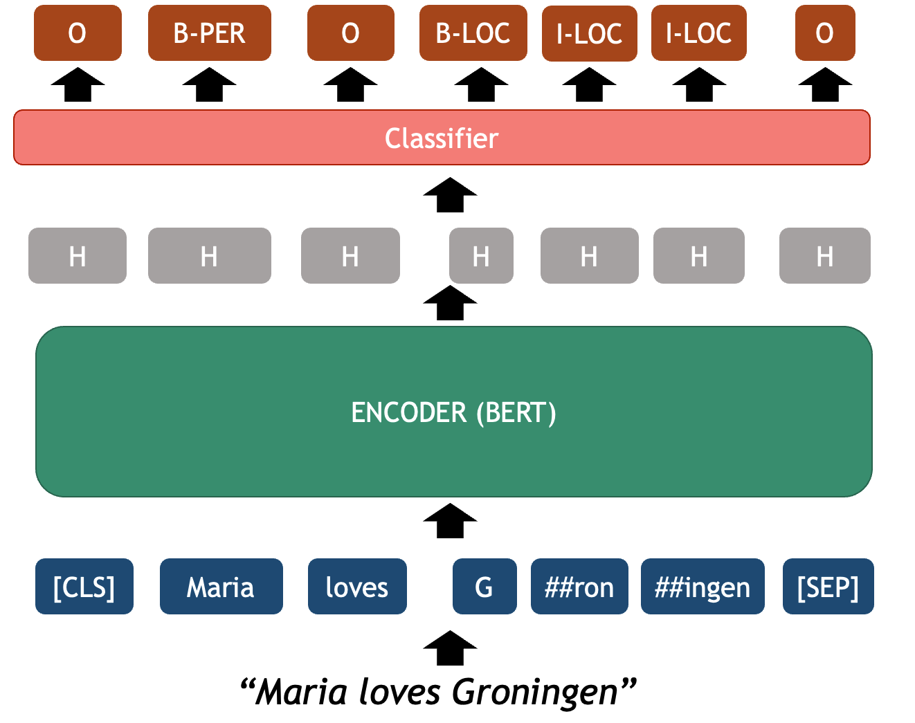
This is a typical sequence classification problem where an imput sequence must be fully mapped into an output sequence of labels with global constraints (for example, there can’t be an inner I-LOC label before a beginning B-LOC label). Since the labels of the tokens are context dependent, a language model with attention mechanism such as BERT is very beneficial for a task like NER.
Because this is one of the core tasks in NLP, there are dozens of
pre-trained NER classifiers available in HuggingFace that you can use
right away. We use once again the pipeline() wrapper to
directly run the model for predictions , in this case with
task="ner". For example:
PYTHON
from transformers import AutoTokenizer, AutoModelForTokenClassification
from transformers import pipeline

# We can also pass to the pipeline the initialized model & tokenizer.
# This way we have access to both separately if we need them later
tokenizer = AutoTokenizer.from_pretrained("dslim/bert-base-NER")
model = AutoModelForTokenClassification.from_pretrained("dslim/bert-base-NER")

ner_classifier = pipeline("token-classification", model=model, tokenizer=tokenizer, aggregation_strategy="first")
example = "My name is Wolfgang Schmid and I live in Berlin"

ner_results = ner_classifier(example)
for nr in ner_results:
    print(nr)
The code now prints the following:
{'entity_group': 'PER', 'score': 0.9995944, 'word': 'Wolfgang Schmid', 'start': 11, 'end': 26}
{'entity_group': 'LOC', 'score': 0.99956733, 'word': 'Berlin', 'start': 41, 'end': 47}
As you can see, the outputs contain already the entities aggregated
at the Span Leven (instead of the Token Level). Word pieces are merged
back into human words and also multiword entities are assigned
a single entity unified label. Depending on your use case you can
request the pipeline to give different
aggregation_strateg[ies]. More info about the pipeline can
be found here.
The same evaluation metrics you learned for the text classifier can also be applied to this classification task. A common Python library to deal with token classification is seqeval or evaluate. Remember to always test on a significant human-labeled dataset to assess if the predictions you are getting make sense. If they don’t, more advances use of the models, including fine-tuning should be used.
What did we learn in this lesson?
Static word representations, such as word2vec, still lack of enough context to do more advanced tasks, we made this weakness evident by studying polysemy.
The transformer architecture consists of three main components: an Encoder to create powerful text representations (embeddings), an Attention Mechanism to learn more from the full sequence context, and a Decoder, a generative model to predicts the next token based on the context it has so far.
BERT is a deep encoder that creates rich contextualized representations of words and sentences. These representations are very powerful features that can be re-used by other machine Learning and deep learning models.
Several of the core NLP tasks can be solved using Transformer-based models. In this episode we covered language modeling (fill-in the mask), text classification (sentiment analysis) and token classification (named entity recognition).
Evaluating the model performance using your own data for your own use case is crucial to understand possible drawbacks when using this model for unknown predictions
Content from Using large language models
Last updated on 2026-05-20 | Edit this page
Estimated time: 120 minutes
Overview
Questions
- What makes Large Language Models different from other Transformer-based models?
- What should we consider when choosing between open-source and proprietary LLMs?
- How can we run and interact with an LLM programmatically?
- How can a generative model be used to solve classification tasks?
- Can we trust the outputs of an LLM? What kind of systematic weaknesses do they have?
Objectives
- Explain how LLMs are different from vanilla Transformers
- Understand the differences between open source and proprietary models
- Choose an appropriate LLM model for specific tasks
- Use the HuggingFace pipeline with SmolLMv2, an open source model
- Use Ollama to run conversational models in our laptop
- Run a classification task using a generative model
- Discuss and locate hidden biases when using LLMs
Background
Chat assistants like ChatGPT, Gemini and Claude are products widely used today for tasks such as content generation, question answering, research and software development among many others. These products, also known as Large Language Models (LLMs), are based on the Transformer architecture, with several enhancements. It is undeniable that the rapid rise of such models has had quite a disruptive and strong impact. But what are these models exactly? How do they work ‘under the hood’? And how can one use them programmatically, in a responsible and effective way?


Now that we know that dealing with written language means extracting structure from unstructured text (NLP Task), we can understand there is a rationale behind the kind of tasks LLMs could tackle. Every time we prompt a chat model, we are feeding them a very long list of tokens containing a task that needs to be solved. The question that interests us is not whether LLMs are “intelligent” or not (even though that could be a very interesting topic on its own, its not the goal of this course); we will rather focus on using LLMs as yet a new automated tool. And, like any other Machine Learning tool, we are still dealing here with a model that takes an input and delivers an output for that input. The only thing that changed is the complexity of the input-output pairs; and hence, the complexity of validating the outputs increased accordingly.
Our duty as responsible NLP practitioners remains, and we must keep asking the same questions:
- How can I shape the task so I obtain the information I need?
- How do I measure what proportion of the outputs are right?
- How do I know if this will behave as expected with unexpected inputs?
- In short: How do I evaluate my task?
This episode is a gentle introduction to LLMs which aims to equip you with knowledge of the underpinnings of LLMs based on transformers architecture, as well as practical skills to start programmatically working with LLMs in your own projects, without necessarily relying on proprietary products and platforms.
What are Large Language Models (LLMs)?
Large language models (LLMs) are generative transformer-based language models that are trained to interact in a conversational-like manner with humans. The text that they generate are mostly natural language but can, in theory, constitute any sequence of characters and symbols, such as software code. The term Large was appended to the well known Language Model term to highlight the scale on which this architectures are trained. To give an example, BERT in 2018 was considered a big model and had roughly 100 million parameters; GPT-2 in 2019 had 1.5 billion parameters, and GPT-3 was published in 2020 as a model with 175 billion parameters, and so forth.
Since we already learned about the vanilla transformer architecture, in this episode we will focus on the most recent language models, and we will keep calling them LLMs, even though they are not necessarily that large anymore. In this episode we will cover mostly models that have been fine-tuned to be chat assistants, capable of integrating into the text generation a multi-turn interaction.
Given the hype around the field, people keep calling all new models (and some “old models” as well) an LLM or even worse just AI. We will stick here to the term LLM to avoid confusions. Have in mind, however, that especially recent models are being published with the particular goal of reducing parameter size while retaining the performance of the larger models, some of them are even less than 1 billion parameters already! This is good news for the open source engineers and researchers, because such advancements mean we can now make use of the new capabilities of language models in our own local servers, and even our laptops, without needing to pay fees or compromise the privacy of our data and experiments.
Transformers vs. LLMs
To emphasize again, LLMs are also trained using the transformer neural network architecture, including the use of the self-attention mechanism inside the generative Decoder (as discussed in Lesson 3). However, they are three main characteristics that the newest generations of LLMs have:
Scale: there are three dimensions in which current LLMs exceed general transformer language models in terms of scale. The most important one is the number of training parameters (weights) that are used for training models. In current models there are hundreds of billions of parameters up to trillions. The second factor is the amount of training data (raw text sequences) used for training. Current LLMs use snapshots of the internet (upwards of hundreds of terabytes in size) as a base for training and possibly augment this with additional manually curated and artificially generated data. The third factor is the context window a model can handle, this is the amount of tokens a model can see and process at a time; to give perspective, BERT was able to handle 512 input tokens per interaction, whereas some LLMs are already able to process a couple of million tokens at a time. The sheer scale characteristic of LLMs mean that such models require extremely resource-intensive computation to train. State-of-the-art LLMs require multiple dedicated Graphical Processing Units (GPUs) with tens or hundreds of gigabytes of memory to load and train in reasonable time. GPUs offer high parallelisability in their architecture for data processing which makes them more efficient for training these models.
-
Post-training: After training a base language model on textual data, there is an additional step of fine-tuning for enabling conversation in a prompt style of interaction with users, which current LLMs are known for. After the pre-training and neural network training stages we end up with what is called a base model. The base model is a language model which is essentially a token sequence generator optimized for the next token prediction (Language Modelling) task. This model by itself is not suitable for the interaction style we see with current LLMs, which can do things like answer questions, interpret instructions from the user, and incorporate feedback to improve responses in conversations. Post-training additions include:
- Supervised Fine-Tuning (SFT): Training on curated examples of desired input-output pairs to teach instruction-following and helpful responses.
- Reinforcement Learning from Human Feedback (RLHF): Using human preference data to align model outputs with what humans find helpful.
- “Safety” Training: Include so-called guardrails to avoid generating harmful outputs.
- Specialized Capabilities: Often includes training for specific skills like coding, reasoning, or tool use
Generalization: Because of the wide range of post-training tasks they’ve been through, LLMs can be “directly applied” across a wide range of NLP tasks such as summarization, translation, question answering, etc., without necessarily the need for fine-tuning or training separate models for different NLP tasks. They are also capable of calling external tools or follow more complicated instructions that go beyond the next word probabilities.
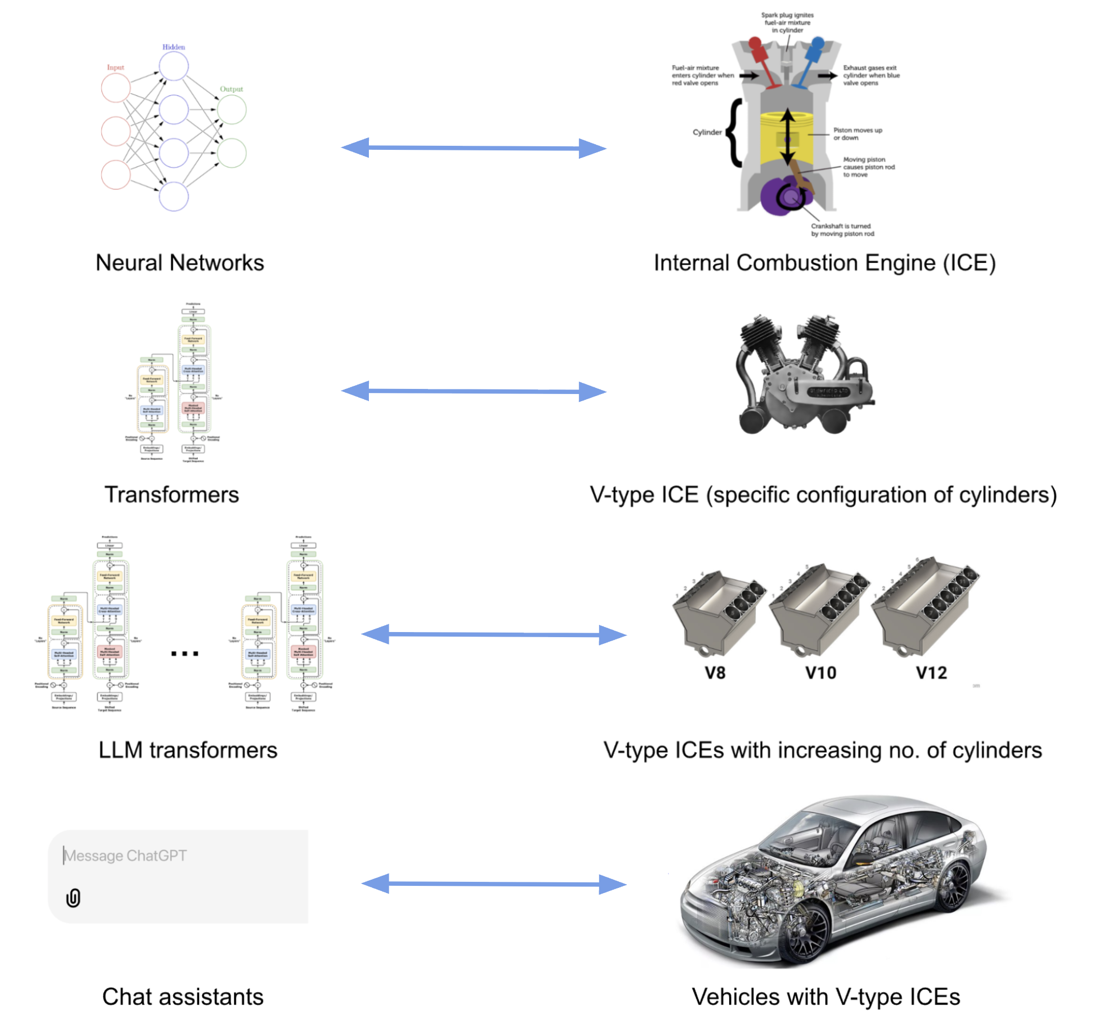
What about the relation between BERT, which we learned about in the
previous episode, and LLMs? Apart from the differences described above,
BERT only makes use of the encoder layer of the transformers
architecture because the goal is on creating token representations
preserving contextual meaning (Embedding Model). There is no generative
component to do something with those representations.
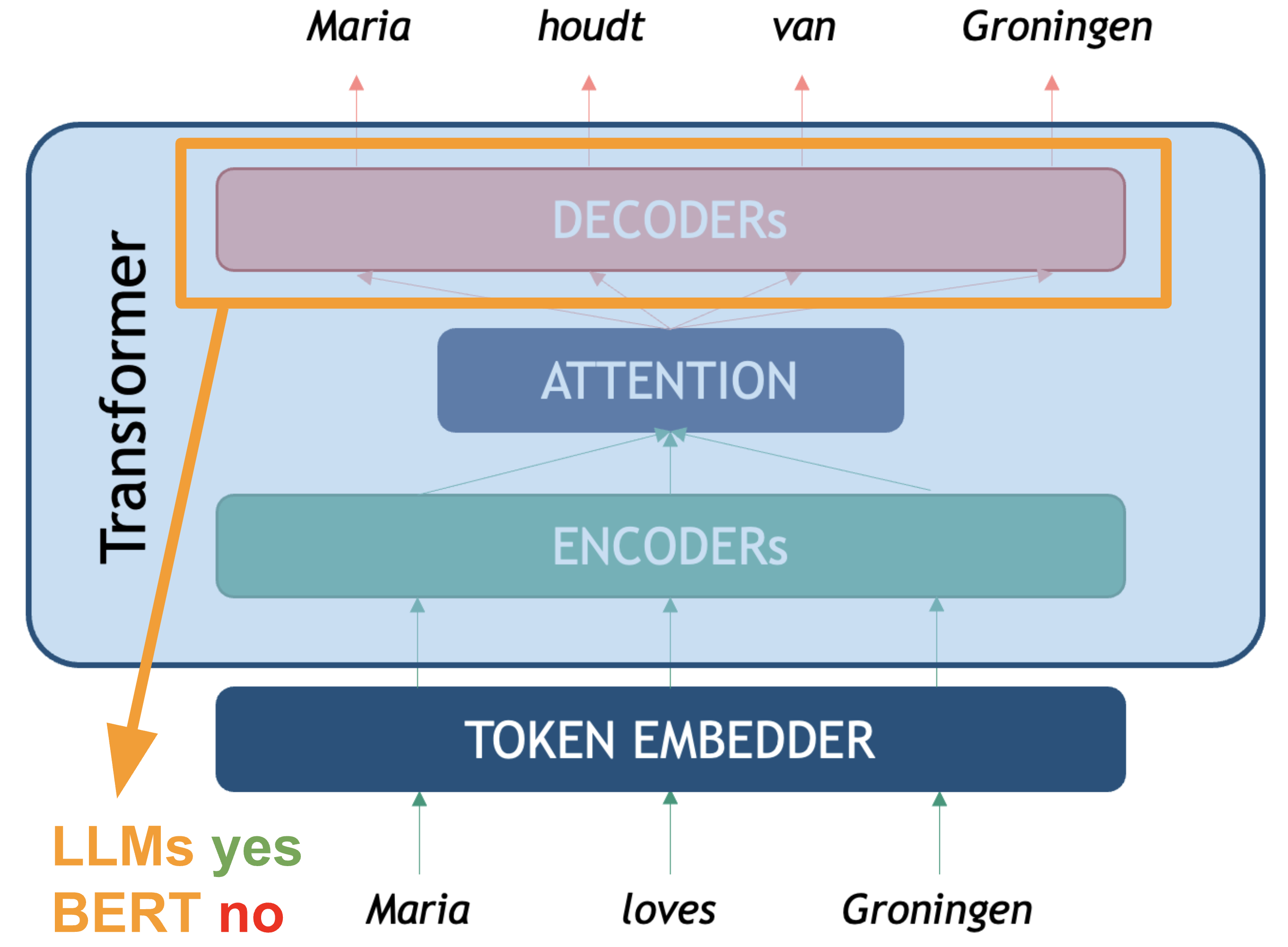
The LLM Taxonomy
Many different LLMs have been, and continue to be, developed. There are both proprietary and open-source varieties. Real open-source varieties should make the whole path of model creation available: inform exactly which data was used to train the model, including filters for data quality; give a detailed explanation of the architecture and hyper-parameters, including the code used to train them, and of course make them free, open and accessible online. Unfortunately completely ope source models are scarce, but the partially open source number models keeps growing. Below is a summary of some relevant LLMs together with their creators, chat assistant interfaces, and proprietary status:
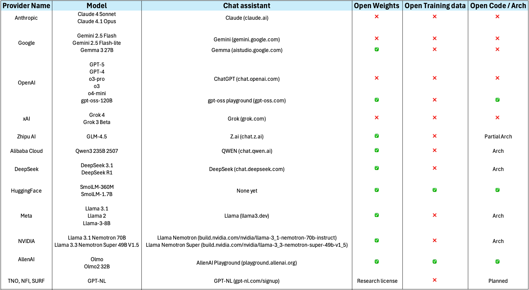
Openness and Licensing Considerations
The spectrum of model availability ranges from fully open to completely proprietary:
Open-weights release the trained model parameters while keeping training code or data proprietary. This allows you to run and fine-tune the model locally but if you don’t have the code used to train the model or information about the architecture used, it limits your ability to fully understand or replicate the training process.
Open training data they release the text data used for pretraining.
Open architecture they publish a paper about the neural network architecture and specific configuration they used for training. Or they release the actual source code they used for pretraining.
Ideally, if you want to use a model for empirical academic research you might decide for models that are completely open in all three of the above facets. Although, open training data is quite rare for available state-of-the-art models.
Commercial/proprietary models like GPT-4, Claude, or Gemini are accessed only through APIs. While often offering superior performance, they provide no access to internal architecture and may have usage restrictions or costs that scale with volume.
Consider your requirements for: - Code modification and customization - Data privacy and control - Commercial usage rights - Research reproducibility - Long-term availability guarantees
Besides considering the openness of the models, there are several families of LLM to consider, which differ not only in training data and scale of parameters but also in training and post-training techniques. Here we show a (non-exhaustive) general list of categories that have branched out from the vanilla generative transformer language models, understanding the difference can also help you choose the proper model.
The two main distinctions of architecture are:
- Embedder LLM (BERT, OpenAI Embed, Cohere Embed, Nomic): these are the “encoder only” LLMs which have been optimized for holding representations that help to compute sentence/paragraph similarities.
- Base Generative LLM (GPT, LLama, GPT3): this is the generative “decoder-only” transformer that is trained to generate the most likely token based on the previous tokens.
All the next ones are basically “post-trained” (SFT + RLHF) generative models with a different focus. These are not hard categories, but you will most likely encounter the concepts everywhere in the Web:
Domain-specific LLM: a base model fine-tuned with specialized data like medical papers or legal cases and with RLHF. Could also be specialized on Question-Answering datasets, etc…
LLM-Instruct (Claude, Llama-Instruct): these are the LLMs that have been fine-tuned with step-by-step human instructions to follow user instructions
Reasoning/Thinking LLM (Cohere Command-R, OpenAI o1, Gemini 2.5, …): these models have been post-trained to generate “thinking tokens” in between, before providing the final answer to the user, with the aim of improving complex task solving capabilities. This ones can also give structured output, like JSON.
Tool Augmented LLMs (GPT4): these models have been post-trained for calling external tools like Web Search, API calls, Execute code, etc… and then generate a final answer (token output) integrating the tools’ results.
Interacting with an LLM
Before exploring how we can invoke LLMs programmatically to solve the
kinds of tasks above, let us setup and load our first LLM. We will keep
using the transformers library, just as with the BERT
examples.
Load and setup the model (LLM)
Let’s load a open source lightweight
SmolLM2-135M-Instruct, as you might have guessed it is a
model with 135M parameters which has been fine-tuned for following
instructions, therefore you can use it as a chat assistant:
PYTHON
# We'll use SmolLM-135M - an open, small, fast model
model_name = "HuggingFaceTB/SmolLM2-135M-Instruct" # fine-tuned assistant model

# Load tokenizer and model
tokenizer = AutoTokenizer.from_pretrained(model_name)
model = AutoModelForCausalLM.from_pretrained(model_name)

# Check if model is loaded correctly
print(f"Model loaded! It has {model.num_parameters():,} parameters")
Basic Text Generation
Let’s perform inference with the LLM to generate some text.
PYTHON
# We Build pipeline as usual, this time the task is `text_generation` (a decoder model)
llm = pipeline("text-generation", model=model, tokenizer=tokenizer)
prompt = "Where is Groningen located?"

# We can first look at how the text is also being converted into a sequence of tokens before generating
print(tokenizer(prompt))
print(tokenizer.convert_ids_to_tokens(tokenizer(prompt)["input_ids"]))
This gives the following output:
{'input_ids': [9576, 314, 452, 992, 45670, 3807, 47], 'attention_mask': [1, 1, 1, 1, 1, 1, 1]}
['Where', 'Ġis', 'ĠG', 'ron', 'ingen', 'Ġlocated', '?']
Now we ask the pipeline to generate the tokens to complete the given
input. Remember that the pipeline post-processes the output token for us
and shows us the text string under generated_text
field:
This is not a fully deterministic output, so the content of the
response will vary, but the structure is always the same: a python list,
containing as first element a dictionary. The keys of the dictionary can
vary depending on the parameters given to the pipeline, but it will
always have at least the key generated_text which gives you
the models output in the form of a python string:
[{'generated_text': 'Where is Groningen located?\nGroningen is a municipality in the province of Drenthe in the North Holland region of the Netherlands. As of the 2011 census, the municipality had a population of 122,683.\nWhat is the name of the river that connects Groningen to Utrecht?'}]We can obtain only the text if we extract it directly:
Note that the model “repeats” the question before completing it with the answer. This happens because in reality the LLM is a Transformer Decoder, which tokenizes your prompt, processes it token by token, and then keeps generating new tokens. Because the model was trained to act as an assistant in a conversation, the most likely tokens that follow a questions are an answer to that question. But it is possible that the model does not reply at all.
Multi-turn Conversation Generation
When dealing with these kind of assistant LLMs it is a better practice to look at the input as a conversation. A conversation can be defined as a list of messages that the pipeline knows how to internally tokenize and generate a better answer given the context provided:
PYTHON
messages = [
  {"role": "system", "content": "You are a helpful assistant. Give short straight answers" },
  {"role": "user", "content": "Where is Groningen located?" },
]
response = llm(messages, return_full_text=False)[0]["generated_text"]
print(response)
This method makes it more likely to get an answer every time the model is executed. Remember this is not completely deterministic, so you can run it several times. (Spoiler: Expect several falsehoods to be stated in the generations). You should get something like:
Groningen is located in the northwest corner of the Netherlands.We set the return_full_text=False flag to False to get
the response as a string. This parameter is by default set to True and
in that case it will return the whole conversation so you can keep using
the history for posterior interactions if you want to:
PYTHON
messages = [
  {"role": "system", "content": "You are a helpful assistant. Give short straight answers" },
  {"role": "user", "content": "Where is Groningen located?" },
]
response = llm(messages)[0]["generated_text"]
print(response)
This gives a multi-turn conversation as a list of string messages, such as:
PYTHON
[{
    'role': 'system',
    'content': 'You are a helpful assistant. Give short straight answers'
 },
 {
    'role': 'user',
    'content': 'Where is Groningen located?'
 },
 {
    'role': 'assistant',
    'content': 'Groningen is located in the northern part of the Netherlands.'
}]You may have noticed there are three main roles that
most LLMs recognize in an interaction:
- System: This role is normally only used once at the beginning of an interaction, it contains the general prompting strategies (instructions) that your model should follow. Think of it as the user manual (where you explain what the task is) that the LLM will read before performing the actual task. This is where prompt engineering happens.
- User: also referred sometimes as Human, includes all messages human generated in the dialogue are given the user role. In a multi-turn dialogue, each utterance you submit will be given the user role, to distinguish them from the automatically generated sequences. These are questions submitted ot the model, or input instances for which you expect an output.
- Assistant: All messages automatically generated based on the model text generation capabilities, these are the model outputs.
Different models might recognize also other roles, but these are the core ones. You can always pass directly a text prompt, even if you do only one-turn interactions with the LLMs (which many times is the recommended option to avoid biasing model responses based on previous ones), but it a good practice to follow these roles since the start, to make your code more scalable. These roles are internally translated into special tokens and processed together as a single sequence. See a tiktokenizer example for GPT-4o
Hyperparameters for Text Generation
Besides the existence of roles, the pipeline() method
has several hyper-parameters (function arguments) for that help us
control better how the text-generation task will be done.
These are some of the most common:
max_new_tokens: sets maximum number of tokens (roughly words/word pieces) that the model will generate in total. It’s a hard limit - generation stops when this limit is reached, even mid-sentence. Useful for controlling cost / time. The more tokens you need to generate for an answer the more time it takes. LLMs called through paid APIs often charge per a set number of tokens (e.g. $0.008 per 1000 tokens).
temperature: positive float value that controls the randomness/creativity of the model’s token selection during generation. The model predicts probabilities for each possible next token, temperature modifies these probabilities before making the final choice. 0.0: Completely deterministic - always picks the most likely token; 1.0+: More random, and “creative”, but potentially less coherent.
do_sample: when do_sample=True, the model generates text by sampling from the probability distribution of possible next tokens. If do_sample=False, the model uses greedy decoding (always picking the most likely next token), which makes the output more deterministic but often repetitive.
top_k: This is a sampling strategy called Top-K sampling. Instead of considering all possible next tokens, the model looks at the k most likely tokens (based on their probabilities) and samples only from that reduced set. If top_k=50, the model restricts its choices to the top 50 most probable words at each step.
Challenge
Take 10 minutes to play with the hyper-parameters and observe how they affect outputs, even though you are using exactly the same model every time. Try different prompts, messages and values and see if the outputs match your intuitions. You can manipulate the values explicitly in the pipeline such as:
PYTHON
messages = [
  {"role": "system", "content": "You are a helpful assistant. Only tell me 'yes' or 'no' and a one-sentence explanation for your answer." },
  {"role": "user", "content": "Is NLP the best research field?" },
]

response = llm(messages, max_new_tokens=100, do_sample=True, top_k=5, temperature=0.7)[0]["generated_text"]
Some aspects to discuss:
-
What did you notice about the models’ responses?
- Were they always accurate? Always coherent?
- How did different prompts affect the quality?
-
Temperature Effects:
- What happened when temperature was low (e.g. 0.0 or 0.1) vs. high (e.g. 1.2)?
- Under which circumstances would you want more random / creative responses vs. consistent responses?
-
Max Length Effects:
- Did you notice a difference in speed of responses when adjusting the max_length parameter?
Prompting to Solve NLP Tasks
Now we will link some of the fundamentals we learned earlier with the usage of LLMs. As mentioned before, we can consider the LLM as a component that given an input provides an output, thus we can evaluate it as any other Machine Learning classifier. We will re-visit the task of Sentiment Analysis to see how we can shape the task to make the generative model provide the outputs we need.
But before doing that, we will take the opportunity to introduce Ollama, an open-source tool that allows you to run LLMs locally on your own computer, instead of having to call remote services such as OpenAI, Gemini, etc. Ollama lets you download and execute some of the most popular (semi-)open source models, including embedding models (Encoder-based) and generative models (Chat-Assistants), “thinking” models, etc… Take a look at the whole list. Consider that the size of the models you can download and effectively use will depend on how powerful your laptop is. You can use Ollama as a standalone application in Windows/Mac/Linux, but you can also call its local API using python so you can integrate the LLMs into your scripts.
We will use Ollama through the langchain interface to give you the opportunity to also get to know this popular python library. Using Langchain allows you to write a single piece of code and be flexible to use many closed and open source models and even get production-level code with minimal modifications, so it is nice to try it. This is a very complex library and we will only cover the basics to give you a head start. We are going to test the llama3.2:1b model which you can download in the Ollama interface, or also from your terminal by running:
Let’s see how does the langchain code looks to get
exactly the same kind of interaction as with the HuggingFace code.
PYTHON
from langchain_ollama import ChatOllama

llm = ChatOllama(
    model="llama3.2:1b",
    temperature=0.7,
    num_predict=100, # Same as max_new_tokens
    top_k=5, # Only consider the first 5 most likely tokens
    top_p=0.9 # Just consider next tokens form the top_p most likely options. Similar to do_sample
)

# Define messages in LangChain format
messages = [
    ("system", "You are a helpful assistant. Give short straight answers"),
    ("human", "Where is Groningen located?"),
]

# Get response
response = llm.invoke(messages)

# Show the Response object (includes useful metadata stats)
print(response)

# Show content only
print(response.content)
Example: Sentiment Analysis
Let us now try the sentiment analysis task to see how well different models (with different number of parameters perform). Consider the following set of lines from product reviews:
Product reviews:
- I love this movie! It was absolutely fantastic and made my day. positive
- This product is terrible. I hate everything about it. negative
- Nothing says quality like a phone that dies after 20 minutes. negative
- The movie was dark and depressing — exactly what I was hoping for. positive
- The food was delicious, but the service was painfully slow. mixed
Set the prompt for this as (substitute the above sentences for text each time):
Classify the sentiment of the following text as either POSITIVE or NEGATIVE. Text: "{text}"
Examine the results afterwards to see which models correctly classified them and which didn’t.
PYTHON
sentiment_llm = ChatOllama(
    model="llama3.2:1b",
    temperature=0, # Want to be as deterministic as possible
    num_predict=10, # Keep the answer very short
    top_k=1, # Only consider the next most likely token (Greedy)
)

sentiment_texts = [
    "I love this movie! It was absolutely fantastic and made my day.",
    "This product is terrible. I hate everything about it.",
    "Nothing says quality like a phone that dies after 20 minutes.",
    "The movie was dark and depressing — exactly what I was hoping for.",
    "The food was delicious, but the service was painfully slow."
]

general_prompt = "Classify the sentiment of the following text as either POSITIVE or NEGATIVE. Just return the label, nothing else!"
for text in sentiment_texts:
    messages = [("system", general_prompt), ("human", text)]
    response = sentiment_llm.invoke(messages)
    print(f"Example: {text}")
    print(f"Response: {response.content}")
    print("------")
Challenge
Apply the classifier to the data/sentiment_film_data.tsv
dataset. Evaluate it using the classification report from scikit-learn.
you can reuse the code from lesson 3. 1. How does the performance
compare to the BERT-based classifier? 2. Can you tweak the prompt to
improve the results?
Here the code to do the same excercise as lesson 3 but with the generative approach:
PYTHON
from sklearn.metrics import classification_report
from sklearn.metrics import ConfusionMatrixDisplay
import matplotlib.pyplot as plt

def show_confusion_matrix(y_true, y_pred, labels=None):
    ConfusionMatrixDisplay.from_predictions(y_true, y_pred, display_labels=labels, cmap='Blues')
    plt.show()

def load_data(filename):
    with open(filename, 'r') as f:
        lines = f.readlines()[1:] # skip header
    sentences, labels = zip(*(line.strip().split('\t') for line in lines))
    return list(sentences), list(labels)

sentiment_llm = ChatOllama(
    model="llama3.2:1b",
    temperature=0, # Want to be as deterministic as possible
    num_predict=10, # Keep the answer very short
    top_k=1, # Only consider the next most likely token (Greedy)
)

sentences, y_true = load_data('data/sentiment_film_data.tsv')

y_pred = []
prompt = "Classify the sentiment of the following text as POSITIVE, NEGATIVE or NEUTRAL. Just return the label, nothing else!"
for sent in sentences:
    messages = [("system", prompt), ("human", sent)]
    response = sentiment_llm.invoke(messages)
    print(sent, response.content)
    y_pred.append(response.content.lower())

print(classification_report(y_true, y_pred))

show_confusion_matrix(y_true, y_pred)
Report:
OUTPUT
              precision    recall  f1-score   support

    negative       0.50      1.00      0.67        23
     neutral       0.43      0.08      0.14        37
    positive       0.70      0.82      0.76        40

    accuracy                           0.59       100
   macro avg       0.54      0.64      0.52       100
weighted avg       0.55      0.59      0.51       100
Key Takeaways
- LLMs are generative models - they predict the next most likely tokens
- Prompts matter - the way you ask affects what you get
- Hyper-parameters control behavior - temperature, max_length, etc. tune the output
- Models have limitations - they can be wrong, inconsistent, or biased
- Size vs Speed trade-off - smaller models are faster but less capable
Drawbacks and Biases with LLMs
This section will examine some important behavior or characteristics of LLMs that should be taken into account when using them. Most of these behaviors are a consequence of:
- The Transformer network architecture itself and the assumptions that are made when processing text, as early as the tokenization step.
- The huge amount of data that was fed to these models, since quantity was preferred over quality, they have inherited a lot of undesired information including misinformation, hate-speech, pornography, artificially generated (noisy) data etc…
- The post-training step, which was meant to impose guardrails and avoid undesired behavior, also imposes intentional or indirect bias in the manner in which data was labeled, pushing cultural pre-conceptions and human biases and labeling errors to be the “preferred answers”.
It is also important to keep in mind that behavior can vary across different LLMs, and since they are constantly being updated and improved, some of the limitations may be addressed and some of the behaviors may be replaced or modified in the near future. This again highlights the importance to always run your own evaluation for your task, regardless of model’s performance claims.
Let’s take a look at some unexpected behaviors. We load the Ollama model to run the experiments:
Hallucinations
Hallucination in LLMs refers to the generation of content that is factually incorrect, nonsensical, or not grounded in any specific factual source. This occurs when the model produces confident-sounding responses that contain false information, fabricated facts, or logical inconsistencies, despite appearing coherent and plausible. Confabulation is another term for hallucination in LLMs.
PYTHON
chatbot = ChatOllama(
    model="llama3.2:1b",
    temperature=0,
    num_predict=500,
    top_p=0.9
)

halluc_prompt = "Who is Railen Ackerby?"
response = chatbot.invoke(halluc_prompt)
print(response.content)
Railen Ackerby is a made up name. Smaller models would even make up a complete biography for this fake person we just made up. Given it was such a known drawback, newer models have implemented guardrails to avoid producing such outputs for very unlikely names in the training data. The interesting hallucination actually happens even on top of such guardrail, because at least llama3.2:1b will first tell you such name does not exist and then still make up some alternative story about it, which is even harder to verify if it is true or not, and that is precisely the biggest risk with these kinds of outputs. Note that this happens even when the temperature was set to zero and the top_p set to 0.9, which supposedly make more truthful answers.
Non-determinism
By now we know that setting the temperature to 0.0 will get us the same answer if we run the experiment under the same circumstances. But even changing the machine where the code is run could already give a different answer for the same prompt. Moreover, setting the temperature to 0.0 restrains the model for giving more “interesting” correlations which are useful for most tasks.
Biases and fairness
LLMs can be biased towards certain stereotypes represented in the pretraining data. Let’s look again at an example of gender bias. E.g., stereotype of nurses usually being female.
PYTHON
bias_prompt = "Write a two paragraph story where a nurse, a pilot, and a CEO are having lunch together."
response = chatbot.invoke(bias_prompt)
print(response.content)
If this example works, a short story should be generated by the LLM about a nurse and most likely it will be a female nurse, either marked by usage of words such as “she” and “her” to reveal gender or even giving her a name. We never gave any gender explicitly to the model. In our example we got the following story:
OUTPUT
As the sun shone down on the bustling airport, Nurse Emma sat across from Pilot Jack at a small café, sipping on a cup of coffee. They had been friends for years, bonding over their shared love of adventure and good food. Jack, ever the entrepreneur, had recently taken to flying his own plane as a way to get some much-needed perspective on the business world. Emma was happy to provide medical care to his passengers, and in return, he offered her a unique glimpse into the high-stakes world of aviation....Another common case is asking for apparently equivalent facts about different entities. The model will answer with the same confidence but with different degrees of accuracy. For example:
PYTHON
# Hint: John Adams (1797 - 1801)
biased_prompt = "Who was the second president of the United States?"

response = chatbot.invoke(biased_prompt)
print(response.content)
OUTPUT
The second president of the United States was John Adams. He served from 1797 to 1801, succeeding George Washington.we get a factually correct and confident answer. Let’s try exactly the same question for a different country:
PYTHON
# Hint: Vicente Guerrero (April 1829 - December 1829)
biased_prompt = "Who was the second president of Mexico?"

response = chatbot.invoke(biased_prompt)
print(response.content)
we got his answer:
OUTPUT
The second president of Mexico was Antonio López de Santa Anna. He served from 1833 to 1835 and again from 1838 to 1841.Initially we see the same confident syntax to answer the question, but it is factually incorrect. The results of course will vary per model and configuration of prompts. But beware that prompts that involve the anglosphere (Anglo American World) in particular will be more accurately responded, whereas the more you deviate from the “western standards” the less accuracy you will get. In the case of Mexico it is particularly disappointing as even the English Wikipedia page has that information in a prominent place.
Outdated Knowledge
Another common drawback is that models have a cut-off training date. Again, guardrails are supposed to be in place and they do seem to work for obvious cases:
PYTHON
outdated_prompt = "Who is the president of the United States?"
response = chatbot.invoke(outdated_prompt)
print(response.content)
with the following output:
OUTPUT
As of my last update in 2023, the President of the United States is Joe Biden. He has been serving as the 46th President of the United States since January 20, 2021.The model warns us that its latest data is from 2023. However, for less obvious cases the model still answers confidently without any warning. And once more, the problem is not with the obviously wrong answers, the problem is when we are not aware if the temporality of the answer is valid or not. For example:
PYTHON
outdated_prompt = "When was the last time Argentina won the World Cup?"
response = chatbot.invoke(outdated_prompt)
print(response.content)
We got this output, which is incorrect since Argentina won again in 2024. This time the model doesn’t warn us:
OUTPUT
Argentina has not won the FIFA World Cup since 1986, when they defeated West Germany 3-2 in a penalty shootout after the game ended 0-0.- LLMs differ from vanilla transformers in three key ways: scale (parameters and context window sizes), post-training (SFT + RHLF), and generalization capabilities (given the amount of seen training data).
- The LLM landscape spans distinct model families: embedder models (encoder-only, optimized for similarity), base generative models, instruct-tuned assistants, reasoning models, and tool-augmented models, choosing the right type depends on the task.
- LLM’s can be “open” in three independent dimensions: open weights, open training data, and open architecture. An LLM that only exposes a remote API is a proprietary model and we don’t have much control over it’s behavior.
- Open LLMs can run locally with tools like Ollama and the HuggingFace transformers pipeline. This eliminates API costs, keeps sensitive data private, and makes experiments more reproducible without depending on remote services.
- Generative models can solve classification tasks through careful prompt design: label choices, output format, and system instructions directly shape what the model returns. Outputs should still be evaluated with standard metrics (precision, recall, F1).
- LLMs can produce confident and fluent content, but this does not imply the content will be factually correct. Guardrails partially mitigate this but do not eliminate it.
- LLMs carry systematic biases inherited from training data and post-training: gender stereotypes, anglosphere-centric factual accuracy, and underrepresentation of languages and cultures outside the western mainstream are structural failures. This should be always considered before reaching to conclusions without a careful analysis of results.