Content from Overview of Amazon SageMaker

---

Last updated on 2025-11-07 | Edit this page

Estimated time: 10 minutes

Overview

Questions

• Why use SageMaker for machine learning?

Objectives

• Introduce SageMaker

Amazon SageMaker is a comprehensive machine learning (ML) platform that empowers users to build, train, tune, and deploy models at scale. Designed to streamline the ML workflow, SageMaker supports data scientists and researchers in tackling complex machine learning problems without needing to manage underlying infrastructure. This allows you to focus on developing and refining your models while leveraging AWS’s robust computing resources for efficient training and deployment.

Why use SageMaker for machine learning?

SageMaker provides several features that make it an ideal choice for researchers and ML practitioners:

• High-performance compute only when needed: SageMaker lets you develop interactively in lightweight, inexpensive notebook environments (or your own laptop) and then launch training, tuning, or inference jobs on more powerful instance types only when necessary. This approach keeps costs low during development and ensures you only pay for expensive compute when you’re actively using it.

• Support for custom scripts: Most training and inference scripts can be run using pre-configured estimators or containers that come with popular ML frameworks such as scikit-learn, PyTorch, TensorFlow, and Hugging Face already installed. In many cases, you can simply include a requirements.txt file to add any additional dependencies you need. When you need more control, SageMaker also supports fully custom Docker containers, so you can bring your own code, dependencies, and environments for training, tuning, and inference — all deployed on scalable AWS infrastructure.

• Flexible compute options: SageMaker lets you easily select instance types tailored to your project needs. For exploratory analysis, use a lightweight CPU (e.g., ml.m5.large). For compute-intensive tasks, such as training deep learning models, you can switch to GPU instances for faster processing. We’ll cover instances more in-depth throughout the lesson (and how to select them), but here’s a preview of the the different types:

  • CPU instances (e.g., ml.m5.large — $0.12/hour): Suitable for general ML workloads, feature engineering, and inference tasks.
  • Memory-optimized instances (e.g., ml.r5.2xlarge — $0.65/hour): Best for handling large datasets in memory.
  • GPU instances (e.g., ml.p3.2xlarge — $3.83/hour): Optimized for compute-intensive tasks like deep learning training, offering accelerated processing.
  • For more details, check out the supplemental “Instances for ML” page. We’ll discuss this topic more throughout the lesson.

• Parallelized training and tuning: SageMaker enables parallelized training across multiple instances, reducing training time for large datasets and complex models. It also supports parallelized hyperparameter tuning, allowing efficient exploration of model configurations with minimal code while maintaining fine-grained control over the process.

• Ease of orchestration / Simplified ML pipelines: Traditional high-performance computing (HPC) or high-throughput computing (HTC) environments often require researchers to break ML workflows into separate batch jobs, manually orchestrating each step (e.g., submitting preprocessing, training, cross-validation, and evaluation as distinct tasks and stitching the results together later). This can be time-consuming and cumbersome, as it requires converting standard ML code into complex Directed Acyclic Graphs (DAGs) and job dependencies. By eliminating the need to manually coordinate compute jobs, SageMaker dramatically reduces ML pipeline complexity, making it easier for researchers to quickly develop and iterate on models efficiently.

• Cost management and monitoring: SageMaker includes built-in monitoring tools to help you track and manage costs, ensuring you can scale up efficiently without unnecessary expenses. For many common use cases of ML/AI, SageMaker can be very affordable. For example, training roughly 100 small to medium-sized models (e.g., logistic regression, random forests, or lightweight deep learning models with a few million parameters) on a small dataset (under 10GB) can cost under $20, making it accessible for many research projects.

In summary, Amazon SageMaker is a fully managed machine learning platform that simplifies building, training, tuning, and deploying models at scale. Unlike traditional research computing environments, which often require manual job orchestration and complex dependency management, SageMaker provides an integrated and automated workflow, allowing users to focus on model development rather than infrastructure. With support for on-demand compute resources, parallelized training and hyperparameter tuning, and flexible model deployment options, SageMaker enables researchers to scale experiments efficiently. Built-in cost tracking and monitoring tools also help keep expenses manageable, making SageMaker a practical choice for both small-scale research projects and large-scale ML pipelines. By combining preconfigured machine learning algorithms, support for custom scripts, and robust computing power, SageMaker reduces the complexity of ML development, empowering researchers to iterate faster and bring models to production more seamlessly.

Key Points

• SageMaker simplifies ML workflows by eliminating the need for manual job orchestration.
• Flexible compute options allow users to choose CPU, GPU, or memory-optimized instances based on workload needs.
• Parallelized training and hyperparameter tuning accelerate model development.
• SageMaker supports both built-in ML algorithms and custom scripts via Docker containers.
• Cost monitoring tools help track and optimize spending on AWS resources.
• SageMaker streamlines scaling from experimentation to deployment, making it suitable for both research and production.

Content from Data Storage: Setting up S3

---

Last updated on 2025-10-15 | Edit this page

Estimated time: 20 minutes

Overview

Questions

• How can I store and manage data effectively in AWS for SageMaker workflows?
• What are the best practices for using S3 versus EC2 storage for machine learning projects?

Objectives

• Explain data storage options in AWS for machine learning projects.
• Describe the advantages of S3 for large datasets and multi-user workflows.
• Outline steps to set up an S3 bucket and manage data within SageMaker.

Storing data on AWS

---

Machine learning and AI projects rely on data, making efficient storage and management essential. AWS provides several options for storing data, each with different use cases and trade-offs.

Consult your institution’s IT before handling sensitive data in AWS

When using AWS for research, ensure that no restricted or sensitive data is uploaded to S3 or any other AWS service unless explicitly approved by your institution’s IT or cloud security team. For projects involving sensitive or regulated data (e.g., HIPAA, FERPA, or proprietary research data), consult your institution’s cloud security or compliance team to explore approved solutions. This may include encryption, restricted-access storage, or dedicated secure environments. If unsure about data > classification, review your institution’s data security policies before uploading.

Options for storage: EC2 Instance or S3

---

When working with SageMaker and other AWS services, you have options for data storage, primarily EC2 instances or S3.

What is an EC2 instance?

An Amazon EC2 (Elastic Compute Cloud) instance is a virtual server environment where you can run applications, process data, and store data temporarily. EC2 instances come in various types and sizes to meet different computing and memory needs, making them versatile for tasks ranging from light web servers to intensive machine learning workloads. For example, when you launch a new Jupyter notebook from Sagemaker, this notebook is run on an an EC2 instance configured to run Jupyter notebooks, enabling direct data processing.

When to store data directly on EC2

Using an EC2 instance for data storage can be useful for temporary or small datasets, especially during processing within a Jupyter notebook. However, this storage is not persistent; if the instance is stopped or terminated, the data is erased. Therefore, EC2 is ideal for one-off experiments or intermediate steps in data processing.

Callout

Limitations of EC2 storage

• Scalability: EC2 storage is limited to the instance’s disk capacity, so it may not be ideal for very large datasets.
• Cost: EC2 storage can be more costly for long-term use compared to S3.
• Data Persistence: EC2 data may be lost if the instance is stopped or terminated, unless using Elastic Block Store (EBS) for persistent storage.

What is an S3 bucket?

Storing data in an S3 bucket is generally preferred for machine learning workflows on AWS, especially when using SageMaker. An S3 bucket is a container in Amazon S3 (Simple Storage Service) where you can store, organize, and manage data files. Buckets act as the top-level directory within S3 and can hold a virtually unlimited number of files and folders, making them ideal for storing large datasets, backups, logs, or any files needed for your project. You access objects in a bucket via a unique S3 URI (e.g., s3://your-bucket-name/your-file.csv), which you can use to reference data across various AWS services like EC2 and SageMaker.

Callout

Benefits of using S3 (recommended for SageMaker and ML workflows)

For flexibility, scalability, and cost efficiency, store data in S3 and load it into EC2 as needed. This setup allows:

• Separation of storage and compute: The most essential advantage. Data in S3 remains accessible even when EC2 instances are stopped or terminated, reducing costs and improving workflow flexibility.
• Easy data sharing: Datasets in S3 are easier to share with team members or across projects compared to EC2 storage.
  
• Integration with AWS services: SageMaker, Lambda, and other AWS services can read directly from and write back to S3, streamlining ML workflows.
  
• Scalability: S3 handles large datasets efficiently, enabling storage beyond the limits of an EC2 instance’s disk space.
  
• Cost efficiency: S3 storage is generally lower cost than expanding EC2 disk volumes, and you only pay for the storage you use.
  
• Data persistence: Unlike EC2 storage, which can be lost if an instance is terminated, S3 ensures long-term data availability.

Recommended approach: S3 buckets

---

In order to upload our titanic dataset to an S3 bucket on AWS, we’ll follow the below summary procedure (details follow):

1. Log in to AWS Console and navigate to S3.
2. Create a new bucket or use an existing one.
3. Upload your dataset files.
4. Use the object URL to reference your data in future experiments.

Detailed procedure

1. Sign in to the AWS Management Console

• Log in to AWS Console using your credentials.

2. Navigate to S3

• Type “S3” in the search bar
• Recommended: Select the star icon to save S3 as a bookmark in your AWS toolbar
• Select S3 - Scalable Storage in the Cloud

3. Create a new bucket

• Click Create Bucket and enter a unique name, and note that bucket name must not contain uppercase characters. To easily find this bucket later in our shared AWS account, please use the following naming convention: teamname-yourname-dataname (e.g., sinkorswim-doejohn-titanic).
• Access Control (ACLs): Disable ACLs (recommended).
  • What are ACLs? Access Control Lists (ACLs) define fine-grained permissions at the object level, allowing you to grant specific users or AWS accounts access to individual files in your bucket.
    
  • Why disable them? AWS now recommends managing access through bucket policies and IAM roles, which offer better security and are easier to manage at scale. Unless you have a specific need for ACLs, disabling them is the best practice.
• Public Access: Turn on “Block all public access” (recommended). This setting prevents unauthorized access and accidental data exposure. If you need external access, use IAM policies or signed URLs instead.
• Versioning: Disable unless you need multiple versions of objects (unnecessary for ML Marathon). Enable only if needed, as versioning increases storage costs. Useful when tracking changes to datasets over time but unnecessary for static datasets.
  
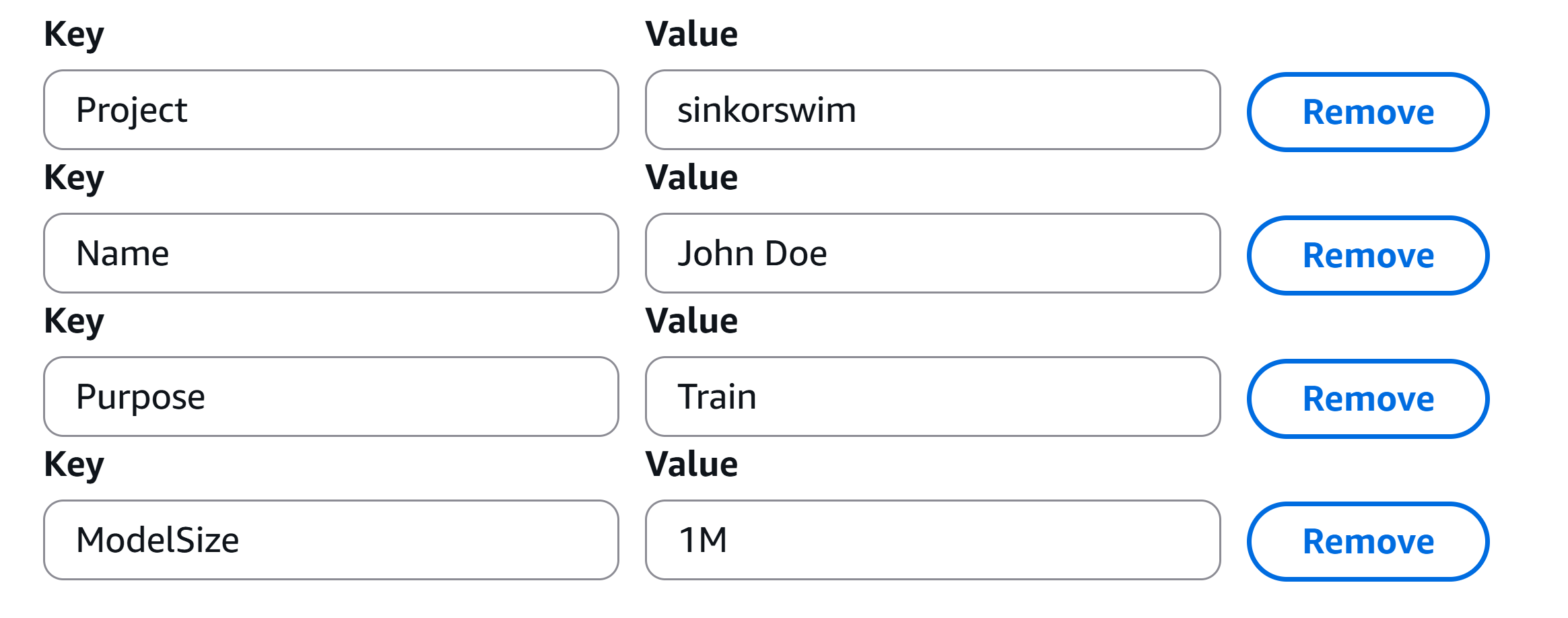
• Tags: Adding tags to your S3 buckets is a great way to track project-specific costs and usage over time, especially as data and resources scale up. To easily track costs associated with your bucket in our shared AWS account, add the following fields:
  • Project: teamname (if participating in ML Marathon)
  • Name: yourname
    • Purpose: Bucket-titanic

Example of Tags for an S3 Bucket

• Click Create Bucket at the bottom once everything above has been configured

4. Edit bucket policy

Once the bucket is created, you’ll be brought to a page that shows all of your current buckets (and those on our shared account). We’ll have to edit our bucket’s policy to allow ourselves proper access to any files stored there (e.g., read from bucket, write to bucket). To set these permissions…

1. Click on the name of your bucket to bring up additional options and settings.
2. Click the Permissions tab
3. Scroll down to Bucket policy and click Edit. Paste the following policy, editing the bucket name “sinkorswim-doejohn-titanic” to reflect your bucket’s name

JSON

{
	"Version": "2012-10-17",
	"Statement": [
		{
			"Effect": "Allow",
			"Principal": {
				"AWS": "arn:aws:iam::183295408236:role/ml-sagemaker-use"
			},
			"Action": [
				"s3:GetObject",
				"s3:PutObject",
				"s3:DeleteObject",
				"s3:ListMultipartUploadParts"
			],
			"Resource": [
				"arn:aws:s3:::sinkorswim-doejohn-titanic",
				"arn:aws:s3:::sinkorswim-doejohn-titanic/*"
			]
		}
	]
}

For workshop attendees, this policy grants the ml-sagemaker-use IAM role access to specific S3 bucket actions, ensuring they can use the bucket for reading, writing, deleting, and listing parts during multipart uploads. Attendees should apply this policy to their buckets to enable SageMaker to operate on stored data.

Callout

General guidance for setting up permissions outside of this workshop

When setting up a bucket outside of this workshop, it’s essential to create a similar IAM role (such as ml-sagemaker-use) with policies that provide controlled access to S3 resources, ensuring only the necessary actions are permitted for security and cost-efficiency.

1. Create an IAM role: Set up an IAM role for SageMaker to assume, with necessary S3 access permissions, such as s3:GetObject, s3:PutObject, s3:DeleteObject, and s3:ListMultipartUploadParts, as shown in the policy above.

2. Attach permissions to S3 buckets: Attach bucket policies that specify this role as the principal, as in our bucket policy above

3. More information: For a detailed guide on setting up roles and policies for SageMaker, refer to the AWS SageMaker documentation on IAM roles and policies. This resource explains role creation, permission setups, and policy best practices tailored for SageMaker’s operations with S3 and other AWS services.

This setup ensures that your SageMaker operations will have the access needed without exposing the bucket to unnecessary permissions or external accounts.

5. Upload files to the bucket

• If you haven’t downloaded these files yet (part of workshop setup), download the data for this workshop: data.zip
  • Extract the zip folder contents (Right-click -> Extract all on Windows; Double-click on mac)
  • Save the two data files (train and test) to a location where they can easily be accessed. E.g., …
    • ~/Downloads/data/titanic_train.csv
    • ~/Downloads/data/titanic_test.csv
• Navigate to the Objects tab of your bucket, then Upload.
• Add Files (titanic_train.csv, titanic_test.csv) and click Upload to complete.

6. Take note of S3 URI for your data

• After uploading a file to S3, click on the file to locate its Object URI (e.g., s3://doejohn-titanic-s3/titanic_train.csv). The Uniform Resource Identifier (URI) is a unique address that specifies the location of the file within S3. This URI is essential for referencing data in AWS services like SageMaker, where it will be used to load data for processing and model training.

S3 bucket costs

---

S3 bucket storage incurs costs based on data storage, data transfer, and request counts.

Storage costs

• Storage is charged per GB per month. Typical: Storing 10 GB costs approximately $0.23/month in S3 Standard (us-east-1).
• Pricing Tiers: S3 offers multiple storage classes (Standard, Intelligent-Tiering, Glacier, etc.), with different costs based on access frequency and retrieval times. Standard S3 fits most purposes.

Data transfer costs

• Uploading data to S3 is free.
• Downloading data (out of S3) incurs charges (~$0.09/GB). Be sure to take note of this fee, as it can add up fast for large datasets.
• In-region transfer (e.g., S3 to EC2) is free, while cross-region data transfer is charged (~$0.02/GB).

Request costs

• GET requests are $0.0004 per 1,000 requests. In the context of Amazon S3, “GET” requests refer to the action of retrieving or downloading data from an S3 bucket. Each time a file or object is accessed in S3, it incurs a small cost per request. This means that if you have code that reads data from S3 frequently, such as loading datasets repeatedly, each read operation counts as a GET request.

To calculate specific costs based on your needs, storage class, and region, refer to AWS’s S3 Pricing Information.

Discussion

Challenge: Estimating Storage Costs

1. Estimate the total cost of storing 1 GB in S3 for one month assuming:

• Storage duration: 1 month
• Storage region: us-east-1
• Storage class: S3 Standard
• Data will be retrieved 100 times for model training and tuning (GET requests)
• Data will be deleted after the project concludes, incurring data retrieval and deletion costs

Hints

• S3 storage cost: $0.023 per GB per month (us-east-1)
• Data transfer cost (retrieval/deletion): $0.09 per GB (us-east-1 out to internet)
• GET requests cost: $0.0004 per 1,000 requests (each model training will incur one GET request)
• Check the AWS S3 Pricing page for more details.

2. Repeat the above calculation using the following dataset sizes: 10 GB, 100 GB, 1 TB (1024 GB)

Show me the solution

Using the S3 Standard rate in us-east-1:

1. 1 GB:
   • Storage: 1 GB * $0.023 = $0.023
   • Retrieval/Deletion: 1 GB * $0.09 = $0.09
     
   • GET Requests: 100 requests * $0.0004 per 1,000 = $0.00004
     
   • Total Cost: $0.11304
2. 10 GB:
   • Storage: 10 GB * $0.023 = $0.23
   • Retrieval/Deletion: 10 GB * $0.09 = $0.90
     
   • GET Requests: 100 requests * $0.0004 per 1,000 = $0.00004
     
   • Total Cost: $1.13004
3. 100 GB:
   • Storage: 100 GB * $0.023 = $2.30
   • Retrieval/Deletion: 100 GB * $0.09 = $9.00
     
   • GET Requests: 100 requests * $0.0004 per 1,000 = $0.00004
     
   • Total Cost: $11.30004
4. 1 TB (1024 GB):
   • Storage: 1024 GB * $0.023 = $23.55
   • Retrieval/Deletion: 1024 GB * $0.09 = $92.16
     
   • GET Requests: 100 requests * $0.0004 per 1,000 = $0.00004
     
   • Total Cost: $115.71004

These costs assume no additional request charges beyond those for retrieval, storage, and GET requests for training.

Removing unused data (complete after the workshop)

---

After you are done using your data, it’s important to practice good resource stewardship and remove the unneeded files/buckets.

Option 1: Delete data only (if you plan to reuse bucket for other datasets)

• Go to S3, navigate to the bucket.
• Select files to delete, then Actions > Delete.

Option 2: Delete the S3 bucket entirely (you no longer need the bucket or data)

• Select the bucket, click Actions > Delete.
• Type the bucket name to confirm deletion.

Please complete option 2 following this workshop. Deleting the bucket stops all costs associated with storage, requests, and data transfer.

Key Points

• Use S3 for scalable, cost-effective, and flexible storage.
• EC2 storage is fairly uncommon, but may be suitable for small, temporary datasets.
• Track your S3 storage costs, data transfer, and requests to manage expenses.
• Regularly delete unused data or buckets to avoid ongoing costs.

Content from Notebooks as Controllers

---

Last updated on 2025-10-09 | Edit this page

Estimated time: 30 minutes

Overview

Questions

• How do you set up and use SageMaker notebooks for machine learning tasks?
• How can you manage compute resources efficiently using SageMaker’s controller notebook approach?

Objectives

• Describe how to use SageMaker notebooks for ML workflows.
• Set up a Jupyter notebook instance as a controller to manage compute tasks.
• Use SageMaker SDK to launch training and tuning jobs on scalable instances.

Setting up our notebook environment

---

Amazon SageMaker provides a managed environment to simplify the process of building, training, and deploying machine learning models. In this episode, we’ll set up a SageMaker notebook instance—a Jupyter notebook hosted on AWS for managing SageMaker workflows.

Using the notebook as a controller

In this setup, the notebook instance functions as a controller to manage more resource-intensive compute tasks. By selecting a minimal instance (e.g., ml.t3.medium), you can perform lightweight operations while leveraging the SageMaker Python SDK to launch scalable compute instances for model training, batch processing, and hyperparameter tuning. This approach minimizes costs while accessing the full power of SageMaker for demanding tasks.

We’ll follow these steps to create our first “SageMaker notebook instance”.

1. Navigate to SageMaker

• In the AWS Console, search for SageMaker.
• Recommended: Select the star icon next to Amazon SageMaker AI to save SageMaker as a bookmark in your AWS toolbar
• Select Amazon SageMaker AI

2. Create a new notebook instance

• In the SageMaker left-side menu, click on Notebooks, then click Create notebook instance.
• Notebook name: To easily track this resource in our shared account, please use the following naming convention: “TeamName-LastnameFirstname-NotebookPurpose”. For example, “sinkorswin-DoeJohn-TrainClassifier”. Can include hyphens, but not spaces.
• Instance type: SageMaker notebooks run on AWS EC2 instances. The instance type determines the compute resources allocated to the notebook. Since our notebook will act as a low-resource “controller”, we’ll select a small instance such as ml.t3.medium (4 GB RAM, $0.04/hour)
  • This keeps costs low while allowing us to launch separate training/tuning jobs on more powerful instances when needed.
    
  • For guidance on common instances for ML procedures, refer to our supplemental Instances for ML webpage.
    
• Platform identifier: This is an internal AWS setting related to the environment version and underlying platform. You can leave this as the default.
• Permissions and encryption:
  • IAM role: For this workshop, we have pre-configured the “ml-sagemmaker-use” role to enable access to AWS services like SageMaker, with some restrictions to prevent overuse/misuse of resources. Select the “ml-sagemmaker-use” role. Outside of the workshop, you create/select a role that includes the AmazonSageMakerFullAccess policy.
  • Root access: Determines whether the user can run administrative commands within the notebook instance. You should Enable root access to allow installing additional packages if/when needed.
    
  • Encryption key (skip): While we won’t use this feature for the workshop, it is possible to specify a KMS key for encrypting data at rest if needed.
• Network (skip): Networking settings are optional. Configure them if you’re working within a specific VPC or need network customization.
• Git repositories configuration (skip): You don’t need to complete this configuration. Instead, we’ll run a clone command from our notebook later to get our repo setup. This approach is a common strategy (allowing some flexiblity in which repo you use for the notebook).
• Tags (NOT OPTIONAL): Adding tags helps track and organize resources for billing and management. This is particularly useful when you need to break down expenses by project, task, or team. To help track costs on our shared account, please use the tags found in the below image.

Tag Setup Example

• Click Create notebook instance. It may take a few minutes for the instance to start. Once its status is InService, you can open the notebook instance and start coding.

Load pre-filled Jupyter notebooks

Once your newly created instance shows as InService, open the instance in Jupyter Lab. From there, we can create as many Jupyter notebooks as we would like within the instance environment.

We will then select the standard python3 environment (conda_python3) to start our first .ipynb notebook (Jupyter notebook). We can use the standard conda_python3 environment since we aren’t doing any training/tuning just yet.

Load pre-filled Jupyter notebooks

Within the Jupyter notebook, run the following command to clone the lesson repo into our Jupyter environment:

SH

!git clone https://github.com/carpentries-incubator/ML_with_AWS_SageMaker.git

Then, navigate to /ML_with_AWS_SageMaker/notebooks/Accessing-S3-via-SageMaker-notebooks.ipynb to begin the first notebook.

Key Points

• Use a minimal SageMaker notebook instance as a controller to manage larger, resource-intensive tasks.
• Launch training and tuning jobs on scalable instances using the SageMaker SDK.
• Tags can help track costs effectively, especially in multi-project or team settings.
• Use the SageMaker SDK documentation to explore additional options for managing compute resources in AWS.

Content from Accessing and Managing Data in S3 with SageMaker Notebooks

---

Last updated on 2025-10-09 | Edit this page

Estimated time: 30 minutes

Overview

Questions

• How can I load data from S3 into a SageMaker notebook?
• How do I monitor storage usage and costs for my S3 bucket?
• What steps are involved in pushing new data back to S3 from a notebook?

Objectives

• Read data directly from an S3 bucket into memory in a SageMaker notebook.
• Check storage usage and estimate costs for data in an S3 bucket.
• Upload new files from the SageMaker environment back to the S3 bucket.

Set up AWS environment

To begin each notebook, it’s important to set up an AWS environment that will allow seamless access to the necessary cloud resources. Here’s what we’ll do to get started:

1. Define the Role: We’ll use get_execution_role() to retrieve the IAM role associated with the SageMaker instance. This role specifies the permissions needed for interacting with AWS services like S3, which allows SageMaker to securely read from and write to storage buckets.

2. Initialize the SageMaker Session: Next, we’ll create a sagemaker.Session() object, which will help manage and track the resources and operations we use in SageMaker, such as training jobs and model artifacts. The session acts as a bridge between the SageMaker SDK commands in our notebook and AWS services.

3. Set Up an S3 Client using boto3: Using boto3, we’ll initialize an S3 client for accessing S3 buckets directly. Boto3 is the official AWS SDK for Python, allowing developers to interact programmatically with AWS services like S3, EC2, and Lambda.

Starting with these initializations prepares our notebook environment to efficiently interact with AWS resources for model development, data management, and deployment.

PYTHON

import boto3
import sagemaker
from sagemaker import get_execution_role

# Initialize the SageMaker role, session, and s3 client
role = sagemaker.get_execution_role() # specifies your permissions to use AWS tools
session = sagemaker.Session() 
s3 = boto3.client('s3')

Preview variable details.

PYTHON

# Print relevant details 
print(f"Execution Role: {role}")  # Displays the IAM role being used
bucket_names = [bucket["Name"] for bucket in s3.list_buckets()["Buckets"]]
print(f"Available S3 Buckets: {bucket_names}")  # Shows the default S3 bucket assigned to SageMaker
print(f"AWS Region: {session.boto_region_name}")  # Prints the region where the SageMaker session is running

Reading data from S3

---

You can either (A) read data from S3 into memory or (B) download a copy of your S3 data into your notebook instance. Since we are using SageMaker notebooks as controllers—rather than performing training or tuning directly in the notebook—the best practice is to read data directly from S3 whenever possible. However, there are cases where downloading a local copy may be useful. We’ll show you both strategies.

A) Reading data directly from S3 into memory

This is the recommended approach for most workflows. By keeping data in S3 and reading it into memory when needed, we avoid local storage constraints and ensure that our data remains accessible for SageMaker training and tuning jobs.

Pros:

• Scalability: Data remains in S3, allowing multiple training/tuning jobs to access it without duplication.
• Efficiency: No need to manage local copies or manually clean up storage.
• Cost-effective: Avoids unnecessary instance storage usage.

Cons:

• Network dependency: Requires internet access to S3.
• Potential latency: Reading large datasets repeatedly from S3 may introduce small delays. This approach works best if you only need to load data once or infrequently.

Example: Reading data from S3 into memory

Our data is stored on an S3 bucket called ‘teamname-name-dataname’ (e.g., sinkorswim-doejohn-titanic). We can use the following code to read data directly from S3 into memory in the Jupyter notebook environment, without actually downloading a copy of train.csv as a local file.

PYTHON

import pandas as pd
# Define the S3 bucket and object key
bucket_name = 'sinkorswim-doejohn-titanic'  # replace with your S3 bucket name

# Read the train data from S3
key = 'titanic_train.csv'  # replace with your object key
response = s3.get_object(Bucket=bucket_name, Key=key)
train_data = pd.read_csv(response['Body'])

# Read the test data from S3
key = 'titanic_test.csv'  # replace with your object key
response = s3.get_object(Bucket=bucket_name, Key=key)
test_data = pd.read_csv(response['Body'])

# check shape
print(train_data.shape)
print(test_data.shape)

# Inspect the first few rows of the DataFrame
train_data.head()

B) Download copy into notebook environment

In some cases, downloading a local copy of the dataset may be useful, such as when performing repeated reads in an interactive notebook session.

Pros:

• Faster access for repeated operations: Avoids repeated S3 requests.
• Works offline: Useful if running in an environment with limited network access.

Cons:

• Consumes instance storage: Notebook instances have limited space.
• Requires manual cleanup: Downloaded files remain until deleted.

Example

PYTHON

!pwd

PYTHON

# Define the S3 bucket and file location
key = "titanic_train.csv"  # Path to your file in the S3 bucket
local_file_path = "/home/ec2-user/SageMaker/titanic_train.csv"  # Local path to save the file

# Initialize the S3 client and download the file
s3.download_file(bucket_name, key, local_file_path)
!ls

Note: You may need to hit refresh on the file explorer panel to the left to see this file. If you get any permission issues…

• check that you have selected the appropriate policy for this notebook
• check that your bucket has the appropriate policy permissions

Check the current size and storage costs of bucket

It’s a good idea to periodically check how much storage you have used in your bucket. You can do this from a Jupyter notebook in SageMaker by using the Boto3 library, which is the AWS SDK for Python. This will allow you to calculate the total size of objects within a specified bucket.

The code below will calculate your bucket size for you. Here is a breakdown of the important pieces in the next code section:

1. Paginator: Since S3 buckets can contain many objects, we use a paginator to handle large listings.
2. Size calculation: We sum the Size attribute of each object in the bucket.
3. Unit conversion: The size is given in bytes, so dividing by 1024 ** 2 converts it to megabytes (MB).

Note: If your bucket has very large objects or you want to check specific folders within a bucket, you may want to refine this code to only fetch certain objects or folders.

PYTHON

# Initialize the total size counter (bytes)
total_size_bytes = 0

# Use a paginator to handle large bucket listings
# This ensures that even if the bucket contains many objects, we can retrieve all of them
paginator = s3.get_paginator("list_objects_v2")

# Iterate through all pages of object listings
for page in paginator.paginate(Bucket=bucket_name):
    # 'Contents' contains the list of objects in the current page, if available
    for obj in page.get("Contents", []):  
        total_size_bytes += obj["Size"]  # Add each object's size to the total

# Convert the total size to gigabytes for cost estimation
total_size_gb = total_size_bytes / (1024 ** 3)

# Convert the total size to megabytes for easier readability
total_size_mb = total_size_bytes / (1024 ** 2)

# Print the total size in MB
print(f"Total size of bucket '{bucket_name}': {total_size_mb:.2f} MB")

# Print the total size in GB
#print(f"Total size of bucket '{bucket_name}': {total_size_gb:.2f} GB")

Using helper functions from GitHub

We have added code to calculate bucket size to a helper function called get_s3_bucket_size(bucket_name) for your convenience. There are also some other helper functions in the AWS_helpers repo to assist you with common AWS/SageMaker workflows. We’ll show you how to clone this code into your notebook environment.

Directory setup

Let’s make sure we’re starting in the root directory of this instance, so that we all have our AWS_helpers.py file located in the same path (/test_AWS/scripts/AWS_helpers.py)

PYTHON

%cd /home/ec2-user/SageMaker/

To clone the repo to our Jupyter notebook, use the following code.

PYTHON

!git clone https://github.com/UW-Madison-DataScience/AWS_helpers.git # downloads AWS_helpers folder/repo (refresh file explorer to see)

Our AWS_helpers.py file can be found in AWS_helpers/helpers.py. With this file downloaded, you can call this function via…

PYTHON

import AWS_helpers.helpers as helpers
helpers.get_s3_bucket_size(bucket_name)

Check storage costs of bucket

To estimate the storage cost of your Amazon S3 bucket directly from a Jupyter notebook in SageMaker, you can use the following approach. This method calculates the total size of the bucket and estimates the monthly storage cost based on AWS S3 pricing.

Note: AWS S3 pricing varies by region and storage class. The example below uses the S3 Standard storage class pricing for the US East (N. Virginia) region as of November 1, 2024. Please verify the current pricing for your specific region and storage class on the AWS S3 Pricing page.

PYTHON

# AWS S3 Standard Storage pricing for US East (N. Virginia) region
# Pricing tiers as of November 1, 2024
first_50_tb_price_per_gb = 0.023  # per GB for the first 50 TB
next_450_tb_price_per_gb = 0.022  # per GB for the next 450 TB
over_500_tb_price_per_gb = 0.021  # per GB for storage over 500 TB

# Calculate the cost based on the size
if total_size_gb <= 50 * 1024:
    # Total size is within the first 50 TB
    cost = total_size_gb * first_50_tb_price_per_gb
elif total_size_gb <= 500 * 1024:
    # Total size is within the next 450 TB
    cost = (50 * 1024 * first_50_tb_price_per_gb) + \
           ((total_size_gb - 50 * 1024) * next_450_tb_price_per_gb)
else:
    # Total size is over 500 TB
    cost = (50 * 1024 * first_50_tb_price_per_gb) + \
           (450 * 1024 * next_450_tb_price_per_gb) + \
           ((total_size_gb - 500 * 1024) * over_500_tb_price_per_gb)

print(f"Estimated monthly storage cost: ${cost:.5f}")
print(f"Estimated annual storage cost: ${cost*12:.5f}")

For your convenience, we have also added this code to a helper function.

PYTHON

monthly_cost, storage_size_gb = helpers.calculate_s3_storage_cost(bucket_name)
print(f"Estimated monthly cost ({storage_size_gb:.4f} GB): ${monthly_cost:.5f}")
print(f"Estimated annual cost ({storage_size_gb:.4f} GB): ${monthly_cost*12:.5f}")

Important Considerations:

• Pricing Tiers: AWS S3 pricing is tiered. The first 50 TB per month is priced at $0.023 per GB, the next 450 TB at $0.022 per GB, and storage over 500 TB at $0.021 per GB. Ensure you apply the correct pricing tier based on your total storage size.
• Region and Storage Class: Pricing varies by AWS region and storage class. The example above uses the S3 Standard storage class pricing for the US East (N. Virginia) region. Adjust the pricing variables if your bucket is in a different region or uses a different storage class.
• Additional Costs: This estimation covers storage costs only. AWS S3 may have additional charges for requests, data retrievals, and data transfers. For a comprehensive cost analysis, consider these factors as well.

For detailed and up-to-date information on AWS S3 pricing, please refer to the AWS S3 Pricing page.

Writing output files to S3

---

As your analysis generates new files or demands additional documentation, you can upload files to your bucket as demonstrated below. For this demo, you can create a blank Notes.txt file to upload to your bucket. To do so, go to File -> New -> Text file, and save it out as Notes.txt.

PYTHON

# Define the S3 bucket name and the file paths
notes_file_path = "Notes.txt" # assuming your file is in root directory of jupyter notebook (check file explorer tab)

# Upload the training file to a new folder called "docs". You can also just place it in the bucket's root directory if you prefer (remove docs/ in code below).
s3.upload_file(notes_file_path, bucket_name, "docs/Notes.txt")

print("Files uploaded successfully.")

After uploading, we can view the objects/files available on our bucket using…

PYTHON

# List and print all objects in the bucket
response = s3.list_objects_v2(Bucket=bucket_name)

# Check if there are objects in the bucket
if 'Contents' in response:
    for obj in response['Contents']:
        print(obj['Key'])  # Print the object's key (its path in the bucket)
else:
    print("The bucket is empty or does not exist.")

Alternatively, we can substitute this for a helper function call as well.

PYTHON

file_list = helpers.list_S3_objects(bucket_name)
file_list

Key Points

• Load data from S3 into memory for efficient storage and processing.
• Periodically check storage usage and costs to manage S3 budgets.
• Use SageMaker to upload analysis results and maintain an organized workflow.

Content from Using a GitHub Personal Access Token (PAT) to Push/Pull from a SageMaker Notebook

---

Last updated on 2025-11-24 | Edit this page

Estimated time: 35 minutes

Overview

Questions

• How can I securely push/pull code to and from GitHub within a SageMaker notebook?
• What steps are necessary to set up a GitHub PAT for authentication in SageMaker?
• How can I convert notebooks to .py files and ignore .ipynb files in version control?

Objectives

• Configure Git in a SageMaker notebook to use a GitHub Personal Access Token (PAT) for HTTPS-based authentication.
• Securely handle credentials in a notebook environment using getpass.
• Convert .ipynb files to .py files for better version control practices in collaborative projects.

Open prefilled .ipynb notebook

---

Open the notebook from: /ML_with_AWS_SageMaker/notebooks/Interacting-with-code-repo.ipynb.

Step 0: Initial setup

---

In this episode, we’ll demonstrate how to push code to GitHub from a SageMaker Jupyter Notebook.

To begin, we will first create a GitHub repo that we have read/write access to. Feel free to supplement the instructions below with your own personal GitHub repo if you have one ou want to use with SageMaker already. Else, we can simply create a fork of AWS_helpers repo. You may have completed this step already if you completed all workshop setup steps.

1. Navigate to https://github.com/UW-Madison-DataScience/AWS_helpers
2. Click the fork button
3. Select yourself as the owner of the fork, and “Copy the main branch only” selected. You will only need the main branch.

Next, let’s make sure we’re starting at the same directory. Back in our SageMaker Jupyter Lab notebook, change directory to the root directory of this instance before going further.

PYTHON

%cd /home/ec2-user/SageMaker/

Then, clone the fork. Replace “USERNAME” below with your GitHub username.

PYTHON

!git clone https://github.com/USERNAME/AWS_helpers.git # replace username with your GitHub username

Step 1: Using a GitHub personal access token (PAT) to push/pull from a SageMaker notebook

---

When working in SageMaker notebooks, you may often need to push code updates to GitHub repositories. However, SageMaker notebooks are typically launched with temporary instances that don’t persist configurations, including SSH keys, across sessions. This makes HTTPS-based authentication, secured with a GitHub Personal Access Token (PAT), a practical solution. PATs provide flexibility for authentication and enable seamless interaction with both public and private repositories directly from your notebook.

Important Note: Personal access tokens are powerful credentials that grant specific permissions to your GitHub account. To ensure security, only select the minimum necessary permissions and handle the token carefully.

Generate a personal access token (PAT) on GitHub

1. Go to Settings by clicking on your profile picture in the upper-right corner of GitHub.
2. Click Developer settings at the very bottom of the left sidebar.
3. Select Personal access tokens, then click Tokens (classic).
4. Click Generate new token (classic).
5. Give your token a descriptive name (e.g., “SageMaker Access Token”) and set an expiration date if desired for added security.
6. Select the minimum permissions needed:
   • For public repositories: Choose only public_repo.
   • For private repositories: Choose repo (full control of private repositories).
   • Optional permissions, if needed:
     • repo:status: Access commit status (if checking status checks).
     • workflow: Update GitHub Actions workflows (only if working with GitHub Actions).
7. Click Generate token and copy it immediately—you won’t be able to see it again once you leave the page.

Caution: Treat your PAT like a password. Avoid sharing it or exposing it in your code. Store it securely (e.g., via a password manager like LastPass) and consider rotating it regularly.

Use getpass to prompt for username and PAT

The getpass library allows you to input your GitHub username and PAT without exposing them in the notebook. This approach ensures you’re not hardcoding sensitive information.

PYTHON

import getpass

# Prompt for GitHub username and PAT securely
username = input("GitHub Username: ")
token = getpass.getpass("GitHub Personal Access Token (PAT): ")

Note: After running, you may want to comment out the above code so that you don’t have to enter in your login every time you run your whole notebook

Step 2: Configure Git settings

---

In your SageMaker or Jupyter notebook environment, run the following commands to set up your Git user information.

Setting this globally (--global) will ensure the configuration persists across all repositories in the environment. If you’re working in a temporary environment, you may need to re-run this configuration after a restart.

PYTHON

!git config --global user.name "Your name" # This is your GitHub username (or just your name), which will appear in the commit history as the author of the changes.
!git config --global user.email your_email@wisc.edu # This should match the email associated with your GitHub account so that commits are properly linked to your profile.

Step 3: Convert json .ipynb files to .py

---

We’d like to track our notebook files within our repo fork. However, to avoid tracking ipynb files directly, which are formatted as json, we may want to convert our notebook to .py first (plain text). Converting notebooks to .py files helps maintain code (and version-control) readability and minimizes potential issues with notebook-specific metadata in Git history.

Benefits of converting to .py before Committing

• Cleaner version control: .py files have cleaner diffs and are easier to review and merge in Git.
• Script compatibility: Python files are more compatible with other environments and can run easily from the command line.
• Reduced repository size: .py files are generally lighter than .ipynb files since they don’t store outputs or metadata.

Here’s how to convert .ipynb files to .py in SageMaker without needing to export or download files.

1. First, install Jupytext.

PYTHON

!pip install jupytext

2. Then, run the following command in a notebook cell to convert both of our notebooks to .py files

PYTHON

# Adjust filename(s) if you used something different
!jupytext --to py Interacting-with-S3.ipynb

SH

[jupytext] Reading Interacting-with-S3.ipynb in format ipynb
[jupytext] Writing Interacting-with-S3.py

3. If you have multiple notebooks to convert, you can automate the conversion process by running this code, which converts all .ipynb files in the current directory to .py files:

PYTHON

import subprocess
import os

# List all .ipynb files in the directory
notebooks = [f for f in os.listdir() if f.endswith('.ipynb')]

# Convert each notebook to .py using jupytext
for notebook in notebooks:
    output_file = notebook.replace('.ipynb', '.py')
    subprocess.run(["jupytext", "--to", "py", notebook, "--output", output_file])
    print(f"Converted {notebook} to {output_file}")

For convenience, we have placed this code inside a convert_files() function in helpers.py.

PYTHON

import AWS_helpers.helpers as helpers
helpers.convert_files(direction="notebook_to_python")

Once converted, move our new .py file to the AWS_helpers folder using the file explorer panel in Jupyter Lab.

Step 4. Add and commit .py files

---

1. Check status of repo. Make sure you’re in the repo folder before running the next step.

PYTHON

%cd /home/ec2-user/SageMaker/AWS_helpers

PYTHON

!git status

2. Add and commit changes

PYTHON

!git add . # you may also add files one at a time, for further specificity over the associated commit message
!git commit -m "Updates from Jupyter notebooks" # in general, your commit message should be more specific!

3. Check status

PYTHON

!git status

Step 5. Adding .ipynb to gitigore

---

Adding .ipynb files to .gitignore is a good practice if you plan to only commit .py scripts. This will prevent accidental commits of Jupyter Notebook files across all subfolders in the repository.

Here’s how to add .ipynb files to .gitignore to ignore them project-wide:

1. Check working directory: First make sure we’re in the repo folder

PYTHON

!pwd
#%cd AWS_helpers

2. Create the .gitignore file: This file will be hidden in Jupyter (since it starts with “.”), but you can verify it exists using ls.

PYTHON

!touch .gitignore
!ls -a

3. Add .ipynb files to .gitignore: You can add this line using a command within your notebook:

PYTHON

with open(".gitignore", "a") as gitignore:
	gitignore.write("\n# Ignore all Jupyter Notebook files\n*.ipynb\n")

View file contents

PYTHON

!cat .gitignore

4. Ignore other common temp files While we’re at it, let’s ignore other common files that can clutter repos, such as cache folders and temporary files.

PYTHON

with open(".gitignore", "a") as gitignore:
	gitignore.write("\n# Ignore cache and temp files\n__pycache__/\n*.tmp\n*.log\n")

View file contents

PYTHON

!cat .gitignore

5. Add and commit the .gitignore file:

Add and commit the updated .gitignore file to ensure it’s applied across the repository.

PYTHON

!git add .gitignore
!git commit -m "Add .ipynb files to .gitignore to ignore notebooks"

This setup will:

• Prevent all .ipynb files from being tracked by Git.
• Keep your repository cleaner, containing only .py scripts for easier version control and reduced repository size.

Step 6. Merging local changes with remote/GitHub

---

Our local changes have now been committed, and we can begin the process of mergining with the remote main branch. Before we try to push our changes, it’s good practice to first to a pull. This is critical when working on a collaborate repo with multiple users, so that you don’t miss any updates from other team members.

1. Pull the latest changes from the main branch

There are a few different options for pulling the remote code into your local version. The best pull strategy depends on your workflow and the history structure you want to maintain. Here’s a breakdown to help you decide:

• Merge (pull.rebase false): Combines the remote changes into your local branch as a merge commit.
  • Use if: You’re okay with having merge commits in your history, which indicate where you pulled in remote changes. This is the default and is usually the easiest for team collaborations, especially if conflicts arise.
• Rebase (pull.rebase true): Replays your local changes on top of the updated main branch, resulting in a linear history.
  • Use if: You prefer a clean, linear history without merge commits. Rebase is useful if you like to keep your branch history as if all changes happened sequentially.
• Fast-forward only (pull.ff only): Only pulls if the local branch can fast-forward to the remote without diverging (no new commits locally).
  • Use if: You only want to pull updates if no additional commits have been made locally. This can be helpful to avoid unintended merges when your branch hasn’t diverged.

Recommended for Most Users

If you’re collaborating and want simplicity, merge (pull.rebase false) is often the most practical option. This will ensure you get remote changes with a merge commit that captures the history of integration points. For those who prefer a more streamlined history and are comfortable with Git, rebase (pull.rebase true) can be ideal but may require more careful conflict handling.

PYTHON

!git config pull.rebase false # Combines the remote changes into your local branch as a merge commit.
!git pull origin main

If you get merge conflicts, be sure to resolve those before moving forward (e.g., use git checkout -> add -> commit). You can skip the below code if you don’t have any conflicts.

PYTHON

# Keep your local changes in one conflicting file
# !git checkout --ours Interacting-with-git.py

# Keep remote version for the other conflicting file
# !git checkout --theirs Interacting-with-git.py

# # Stage the files to mark the conflicts as resolved
# !git add Interacting-with-git.py

# # Commit the merge result
# !git commit -m "Resolved merge conflicts by keeping local changes"

2. Push changes using PAT creditials

PYTHON

# Push with embedded credentials from getpass (avoids interactive prompt)
github_url = f'github.com/{username}/AWS_helpers.git' # The full address for your fork can be found under Code -> Clone -> HTTPS (remote the https:// before the rest of the address)
!git push https://{username}:{token}@{github_url} main

After pushing, you can navigate back to your fork on GitHub to verify everything worked (e.g., https://github.com/username/AWS_helpers/tree/main)

Step 7: Pulling .py files and converting back to notebook format

---

Let’s assume you’ve taken a short break from your work, and others on your team have made updates to your .py files on the remote main branch. If you’d like to work with notebook files again, you can again use jupytext to convert your .py files back to .ipynb.

1. First, pull any updates from the remote main branch.

PYTHON

!git config pull.rebase false # Combines the remote changes into your local branch as a merge commit.
!git pull origin main

2. We can then use jupytext again to convert in the other direction (.py to .ipynb). This command will create Interacting-with-S3.ipynb in the current directory, converting the Python script to a Jupyter Notebook format. Jupytext handles the conversion gracefully without expecting the .py file to be in JSON format.

PYTHON

!jupytext --to notebook Interacting-with-S3.py --output Interacting-with-S3.ipynb

Applying to all .py files

To convert all of your .py files to notebooks, you can use our helper function as follows

PYTHON

helpers.convert_files(direction="python_to_notebook")

Key Points

• Use a GitHub PAT for HTTPS-based authentication in temporary SageMaker notebook instances.
• Securely enter sensitive information in notebooks using getpass.
• Converting .ipynb files to .py files helps with cleaner version control and easier review of changes.
• Adding .ipynb files to .gitignore keeps your repository organized and reduces storage.

Content from Training Models in SageMaker: Intro

---

Last updated on 2025-10-09 | Edit this page

Estimated time: 30 minutes

Overview

Questions

• What are the differences between local training and SageMaker-managed training?
• How do Estimator classes in SageMaker streamline the training process for various frameworks?
• How does SageMaker handle data and model parallelism, and when should each be considered?

Objectives

• Understand the difference between training locally in a SageMaker notebook and using SageMaker’s managed infrastructure.
• Learn to configure and use SageMaker’s Estimator classes for different frameworks (e.g., XGBoost, PyTorch, SKLearn).
• Understand data and model parallelism options in SageMaker, including when to use each for efficient training.
• Compare performance, cost, and setup between custom scripts and built-in images in SageMaker.
• Conduct training with data stored in S3 and monitor training job status using the SageMaker console.

Initial setup

---

1. Open prefilled .ipynb notebook

Open the notebook from: /ML_with_AWS_SageMaker/notebooks/Training-models-in-SageMaker-notebooks.ipynb

2. CD to instance home directory

So we all can reference the helper functions using the same path, CD to…

PYTHON

%cd /home/ec2-user/SageMaker/

3. Initialize SageMaker environment

This code initializes the AWS SageMaker environment by defining the SageMaker role and S3 client. It also specifies the S3 bucket and key for accessing the Titanic training dataset stored in an S3 bucket.

Boto3 API

Boto3 is the official AWS SDK for Python, allowing developers to interact programmatically with AWS services like S3, EC2, and Lambda. It provides both high-level and low-level APIs, making it easy to manage AWS resources and automate tasks. With built-in support for paginators, waiters, and session management, Boto3 simplifies working with AWS credentials, regions, and IAM permissions. It’s ideal for automating cloud operations and integrating AWS services into Python applications.

PYTHON

import boto3
import pandas as pd
import sagemaker
from sagemaker import get_execution_role

# Initialize the SageMaker role (will reflect notebook instance's policy)
role = sagemaker.get_execution_role()
print(f'role = {role}')

# Initialize an S3 client to interact with Amazon S3, allowing operations like uploading, downloading, and managing objects and buckets.
s3 = boto3.client('s3')

# Define the S3 bucket that we will load from
bucket_name = 'sinkorswim-doejohn-titanic'  # replace with your S3 bucket name

# Define train/test filenames
train_filename = 'titanic_train.csv'
test_filename = 'titanic_test.csv'

Create a SageMaker session to manage interactions with Amazon SageMaker, such as training jobs, model deployments, and data input/output.

PYTHON

region = "us-east-2" # United States (Ohio). Make sure this matches what you see near top right of AWS Console menu
boto_session = boto3.Session(region_name=region) # Create a Boto3 session that ensures all AWS service calls (including SageMaker) use the specified region
session = sagemaker.Session(boto_session=boto_session)

4. Get code from git repo (skip if completed already from earlier episodes)

If you didn’t complete the earlier episodes, you’ll need to clone our code repo before moving forward. Check to make sure we’re in our EC2 root folder first (/home/ec2-user/SageMaker).

PYTHON

%cd /home/ec2-user/SageMaker/

PYTHON

# uncomment below line only if you still need to download the code repo (replace username with your GitHub usernanme)
#!git clone https://github.com/username/AWS_helpers.git 

Testing train.py on this notebook’s instance

---

In this next section, we will learn how to take a model training script that was written/designed to run locally, and deploy it to more powerful instances (or many instances) using SageMaker. This is helpful for machine learning jobs that require extra power, GPUs, or benefit from parallelization. However, before we try exploiting this extra power, it is essential that we test our code thoroughly! We don’t want to waste unnecessary compute cycles and resources on jobs that produce bugs rather than insights.

General guidelines for testing ML pipelines before scaling

• Run tests locally first (if feasible) to avoid unnecessary AWS charges. Here, we assume that local tests are not feasible due to limited local resources. Instead, we use our SageMaker instance to test our script on a minimally sized EC2 instance.
• Use a small dataset subset (e.g., 1-5% of data) to catch issues early and speed up tests.
• Start with a small/cheap instance before committing to larger resources. Visit the Instances for ML page for guidance.
• Log everything to track training times, errors, and key metrics.
• Verify correctness first before optimizing hyperparameters or scaling.

Discussion

What tests should we do before scaling?

Before scaling to mutliple or more powerful instances (e.g., training on larger/multiple datsets in parallel or tuning hyperparameters in parallel), it’s important to run a few quick sanity checks to catch potential issues early. In your group, discuss:

• Which checks do you think are most critical before scaling up?
  
• What potential issues might we miss if we skip this step?

Show me the solution

Which checks do you think are most critical before scaling up?

• Data loads correctly – Ensure the dataset loads without errors, expected columns exist, and missing values are handled properly.
  
• Overfitting check – Train on a small dataset (e.g., 100 rows). If it doesn’t overfit, there may be a data or model setup issue.
  
• Loss behavior check – Verify that training loss decreases over time and doesn’t diverge.
  
• Training time estimate – Run on a small subset to estimate how long full training will take.
• Memory estimate - Estimate the memory needs of the algorithm/model you’re using, and understand how this scales with input size.
• Save & reload test – Ensure the trained model can be saved, reloaded, and used for inference without errors.

What potential issues might we miss if we skip the above checks?

• Silent data issues – Missing values, unexpected distributions, or incorrect labels could degrade model performance.
  
• Code bugs at scale – Small logic errors might not break on small tests but could fail with larger datasets.
  
• Inefficient training runs – Without estimating runtime, jobs may take far longer than expected, wasting AWS resources.
  
• Memory or compute failures – Large datasets might exceed instance memory limits, causing crashes or slowdowns.
  
• Model performance issues – If a model doesn’t overfit a small dataset, there may be problems with features, training logic, or hyperparameters.

Callout

Know Your Data Before Modeling

The sanity checks above focus on validating the code, but a model is only as good as the data it’s trained on. A deeper look at feature distributions, correlations, and potential biases is critical before scaling up. We won’t cover that here, but it’s essential to keep in mind for any ML/AI practitioner.

Discussion

Understanding the XGBoost Training Script

Take a moment to review the AWS_helpers/train_xgboost.py script we just cloned into our notebook. This script handles preprocessing, training, and saving an XGBoost model, while also adapting to both local and SageMaker-managed environments.

Try answering the following questions:

1. Data Preprocessing: What transformations are applied to the dataset before training?

2. Training Function: What does the train_model() function do? Why do we print the training time?

3. Command-Line Arguments: What is the purpose of argparse in this script? How would you modify the script if you wanted to change the number of training rounds?

4. Handling Local vs. SageMaker Runs: How does the script determine whether it is running in a SageMaker training job or locally (within this notebook’s instance)?

5. Training and Saving the Model: What format is the dataset converted to before training, and why? How is the trained model saved, and where will it be stored?

After reviewing, discuss any questions or observations with your group.

Show me the solution

1. Data Preprocessing: The script fills missing values (Age with median, Embarked with mode), converts categorical variables (Sex and Embarked) to numerical values, and removes columns that don’t contribute to prediction (Name, Ticket, Cabin).

2. Training Function: The train_model() function takes the training dataset (dtrain), applies XGBoost training with the specified hyperparameters, and prints the training time. Printing training time helps compare different runs and ensures that scaling decisions are based on performance metrics.

3. Command-Line Arguments: argparse allows passing parameters like max_depth, eta, num_round, etc., at runtime without modifying the script. To change the number of training rounds, you would update the --num_round argument when running the script: python train_xgboost.py --num_round 200

4. Handling Local vs. SageMaker Runs: The script uses os.environ.get("SM_CHANNEL_TRAIN", ".") and os.environ.get("SM_MODEL_DIR", ".") to detect whether it’s running in SageMaker. SM_CHANNEL_TRAIN is the directory where SageMaker stores input training data, and SM_MODEL_DIR is the directory where trained models should be saved. If these environment variables are not set (e.g., running locally), the script defaults to "." (current directory).

5. Training and Saving the Model: The dataset is converted into XGBoost’s DMatrix format, which is optimized for memory and computation efficiency. The trained model is saved using joblib.dump() to xgboost-model, stored either in the SageMaker SM_MODEL_DIR (if running in SageMaker) or in the local directory.

Download data into notebook environment

It can be convenient to have a copy of the data (i.e., one that you store in your notebook’s instance) to allow us to test our code before scaling things up.

Callout

While we demonstrate how to download data into the notebook environment for testing our code (previously setup for local ML pipelines), keep in mind that S3 is the preferred location for dataset storage in a scalable ML pipeline.

Run the next code chunk to download data from S3 to notebook environment. You may need to hit refresh on the file explorer panel to the left to see this file. If you get any permission issues…

• check that you have selected the appropriate policy for this notebook
• check that your bucket has the appropriate policy permissions

PYTHON

# Define the S3 bucket and file location
file_key = f"{train_filename}"  # Path to your file in the S3 bucket
local_file_path = f"./{train_filename}"  # Local path to save the file

# Download the file using the s3 client variable we initialized earlier
s3.download_file(bucket_name, file_key, local_file_path)
print("File downloaded:", local_file_path)

We can do the same for the test set.

PYTHON

# Define the S3 bucket and file location
file_key = f"{test_filename}"  # Path to your file in the S3 bucket. W
local_file_path = f"./{test_filename}"  # Local path to save the file

# Initialize the S3 client and download the file
s3.download_file(bucket_name, file_key, local_file_path)
print("File downloaded:", local_file_path)

Logging runtime & instance info

To compare our local runtime with future experiments, we’ll need to know what instance was used, as this will greatly impact runtime in many cases. We can extract the instance name for this notebook using…

PYTHON

# Replace with your notebook instance name.
# This does NOT refer to specific ipynb files, but to the SageMaker notebook instance.
notebook_instance_name = 'sinkorswim-DoeJohn-TrainClassifier'

# Make sure this matches what you see near top right of AWS Console menu
region = "us-east-2" # United States (Ohio)

# Initialize SageMaker client
sagemaker_client = boto3.client('sagemaker', region_name=region)

# Describe the notebook instance
response = sagemaker_client.describe_notebook_instance(NotebookInstanceName=notebook_instance_name)

# Display the status and instance type
print(f"Notebook Instance '{notebook_instance_name}' status: {response['NotebookInstanceStatus']}")
local_instance = response['InstanceType']
print(f"Instance Type: {local_instance}")

Helper: get_notebook_instance_info()

You can also use the get_notebook_instance_info() function found in AWS_helpers.py to retrieve this info for your own project.

PYTHON

import AWS_helpers.helpers as helpers
helpers.get_notebook_instance_info(notebook_instance_name, region)

Test train.py on this notebook’s instance (or when possible, on your own machine) before doing anything more complicated (e.g., hyperparameter tuning on multiple instances)

PYTHON

!pip install xgboost # need to add this to environment to run train.py

Local test

PYTHON

import time as t # we'll use the time package to measure runtime

start_time = t.time()

# Define your parameters. These python vars wil be passed as input args to our train_xgboost.py script using %run

max_depth = 3 # Sets the maximum depth of each tree in the model to 3. Limiting tree depth helps control model complexity and can reduce overfitting, especially on small datasets.
eta = 0.1 #  Sets the learning rate to 0.1, which scales the contribution of each tree to the final model. A smaller learning rate often requires more rounds to converge but can lead to better performance.
subsample = 0.8 # Specifies that 80% of the training data will be randomly sampled to build each tree. Subsampling can help with model robustness by preventing overfitting and increasing variance.
colsample_bytree = 0.8 # Specifies that 80% of the features will be randomly sampled for each tree, enhancing the model's ability to generalize by reducing feature reliance.
num_round = 100 # Sets the number of boosting rounds (trees) to 100. More rounds typically allow for a more refined model, but too many rounds can lead to overfitting.
train_file = 'titanic_train.csv' #  Points to the location of the training data

# Use f-strings to format the command with your variables
%run AWS_helpers/train_xgboost.py --max_depth {max_depth} --eta {eta} --subsample {subsample} --colsample_bytree {colsample_bytree} --num_round {num_round} --train {train_file}

# Measure and print the time taken
print(f"Total local runtime: {t.time() - start_time:.2f} seconds, instance_type = {local_instance}")

Training on this relatively small dataset should take less than a minute, but as we scale up with larger datasets and more complex models in SageMaker, tracking both training time and total runtime becomes essential for efficient debugging and resource management.

Note: Our code above includes print statements to monitor dataset size, training time, and total runtime, which provides insights into resource usage for model development. We recommend incorporating similar logging to track not only training time but also total runtime, which includes additional steps like data loading, evaluation, and saving results. Tracking both can help you pinpoint bottlenecks and optimize your workflow as projects grow in size and complexity, especially when scaling with SageMaker’s distributed resources.

Sanity check: Quick evaluation on test set

This next section isn’t SageMaker specific, but it does serve as a good sanity check to ensure our model is training properly. Here’s how you would apply the outputted model to your test set using your local notebook instance.

PYTHON

import xgboost as xgb
import pandas as pd
import numpy as np
from sklearn.metrics import accuracy_score
import joblib
from AWS_helpers.train_xgboost import preprocess_data

# Load the test data
test_data = pd.read_csv('./titanic_test.csv')

# Preprocess the test data using the imported preprocess_data function
X_test, y_test = preprocess_data(test_data)

# Convert the test features to DMatrix for XGBoost
dtest = xgb.DMatrix(X_test)

# Load the trained model from the saved file
model = joblib.load('./xgboost-model')

# Make predictions on the test set
preds = model.predict(dtest)
predictions = np.round(preds)  # Round predictions to 0 or 1 for binary classification

# Calculate and print the accuracy of the model on the test data
accuracy = accuracy_score(y_test, predictions)
print(f"Test Set Accuracy: {accuracy:.4f}")

A reasonably high test set accuracy suggests our code/model is working correctly.

Training via SageMaker (using notebook as controller) - custom train.py script

---

Unlike “local” training (using this notebook), this next approach leverages SageMaker’s managed infrastructure to handle resources, parallelism, and scalability. By specifying instance parameters, such as instance_count and instance_type, you can control the resources allocated for training.

Which instance to start with?

In this example, we start with one ml.m5.large instance, which is suitable for small- to medium-sized datasets and simpler models. Using a single instance is often cost-effective and sufficient for initial testing, allowing for straightforward scaling up to more powerful instance types or multiple instances if training takes too long. See here for further guidance on selecting an appropriate instance for your data/model: EC2 Instances for ML

Overview of Estimator classes in SageMaker

To launch this training “job”, we’ll use the XGBoost “Estimator. In SageMaker, Estimator classes streamline the configuration and training of models on managed instances. Each Estimator can work with custom scripts and be enhanced with additional dependencies by specifying a requirements.txt file, which is automatically installed at the start of training. Here’s a breakdown of some commonly used Estimator classes in SageMaker:

1. Estimator (Base Class)

• Purpose: General-purpose for custom Docker containers or defining an image URI directly.
• Configuration: Requires specifying an image_uri and custom entry points.
• Dependencies: You can use requirements.txt to install Python packages or configure a custom Docker container with pre-baked dependencies.
• Ideal Use Cases: Custom algorithms or models that need tailored environments not covered by built-in containers.

2. XGBoost Estimator

• Purpose: Provides an optimized container specifically for XGBoost models.
• Configuration:
  • entry_point: Path to a custom script, useful for additional preprocessing or unique training workflows.
  • framework_version: Select XGBoost version, e.g., "1.5-1".
  • dependencies: Specify additional packages through requirements.txt to enhance preprocessing capabilities or incorporate auxiliary libraries.
• Ideal Use Cases: Tabular data modeling using gradient-boosted trees; cases requiring custom preprocessing or tuning logic.

3. PyTorch Estimator

• Purpose: Configures training jobs with PyTorch for deep learning tasks.
• Configuration:
  • entry_point: Training script with model architecture and training loop.
  • instance_type: e.g., ml.p3.2xlarge for GPU acceleration.
  • framework_version and py_version: Define specific versions.
  • dependencies: Install any required packages via requirements.txt to support advanced data processing, data augmentation, or custom layer implementations.
• Ideal Use Cases: Deep learning models, particularly complex networks requiring GPUs and custom layers.

4. SKLearn Estimator

• Purpose: Supports scikit-learn workflows for data preprocessing and classical machine learning.
• Configuration:
  • entry_point: Python script to handle feature engineering, preprocessing, or training.
  • framework_version: Version of scikit-learn, e.g., "1.0-1".
  • dependencies: Use requirements.txt to install any additional Python packages required by the training script.
• Ideal Use Cases: Classical ML workflows, extensive preprocessing, or cases where additional libraries (e.g., pandas, numpy) are essential.

5. TensorFlow Estimator

• Purpose: Designed for training and deploying TensorFlow models.
• Configuration:
  • entry_point: Script for model definition and training process.
  • instance_type: Select based on dataset size and computational needs.
  • dependencies: Additional dependencies can be listed in requirements.txt to install TensorFlow add-ons, custom layers, or preprocessing libraries.
• Ideal Use Cases: NLP, computer vision, and transfer learning applications in TensorFlow.

6. HuggingFace Estimator

• Purpose: Provides managed containers for running inference, fine-tuning, and Retrieval-Augmented Generation (RAG) workflows using the Hugging Face transformers library.
  
• Configuration:
  • entry_point: Custom script for training or inference (e.g., train.py or rag_inference.py).
    
  • transformers_version, pytorch_version, py_version: Define framework versions.
    
  • dependencies: Optional requirements.txt for extra libraries.
    
• Ideal Use Cases: RAG pipelines, LLM inference, NLP, vision, or multimodal tasks using pretrained Transformer models.

Callout

Configuring custom environments with requirements.txt

For all these Estimators, adding a requirements.txt file as a dependencies argument ensures that additional packages are installed before training begins. This approach allows the use of specific libraries that may be critical for custom preprocessing, feature engineering, or model modifications. Here’s how to include it:

PYTHON

# # Customizing estimator using requirements.txt
# from sagemaker.sklearn.estimator import SKLearn
# sklearn_estimator = SKLearn(
#     base_job_name=notebook_instance_name,
#     entry_point="train_script.py",
#     role=role,
#     instance_count=1,
#     instance_type="ml.m5.large",
#     output_path=f"s3://{bucket_name}/output",
#     framework_version="1.0-1",
#     dependencies=['requirements.txt'],  # Adding custom dependencies
#     hyperparameters={
#         "max_depth": 5,
#         "eta": 0.1,
#         "subsample": 0.8,
#         "num_round": 100
#     }
# )

This setup simplifies training, allowing you to maintain custom environments directly within SageMaker’s managed containers, without needing to build and manage your own Docker images. The AWS SageMaker Documentation provides lists of pre-built container images for each framework and their standard libraries, including details on pre-installed packages.

Deploying to other instances

For this deployment, we configure the “XGBoost” estimator with a custom training script, train_xgboost.py, and define hyperparameters directly within the SageMaker setup. Here’s the full code, with some additional explanation following the code.

PYTHON

from sagemaker.inputs import TrainingInput
from sagemaker.xgboost.estimator import XGBoost

# Define instance type/count we'll use for training
instance_type="ml.m5.large"
instance_count=1 # always start with 1. Rarely is parallelized training justified with data < 50 GB. More on this later.

# Define max runtime in seconds to ensure you don't use more compute time than expected. Use a generous threshold (2x expected time but < 2 days) so that work isn't interrupted without any gains.
max_run = 2*60*60 # 2 hours

# Define S3 paths for input and output
train_s3_path = f's3://{bucket_name}/{train_filename}'

# we'll store all results in a subfolder called xgboost on our bucket. This folder will automatically be created if it doesn't exist already.
output_folder = 'xgboost'
output_path = f's3://{bucket_name}/{output_folder}/' 

# Set up the SageMaker XGBoost Estimator with custom script
xgboost_estimator = XGBoost(
    base_job_name=notebook_instance_name,
    max_run=max_run, # in seconds; always include (max 48 hours)
    entry_point='train_xgboost.py',      # Custom script path
    source_dir='AWS_helpers',               # Directory where your script is located
    role=role,
    instance_count=instance_count,
    instance_type=instance_type,
    output_path=output_path,
    sagemaker_session=session,
    framework_version="1.5-1",           # Use latest supported version for better compatibility
    hyperparameters={
        'train': train_file,
        'max_depth': max_depth,
        'eta': eta,
        'subsample': subsample,
        'colsample_bytree': colsample_bytree,
        'num_round': num_round
    }
)

# Define input data
train_input = TrainingInput(train_s3_path, content_type='csv')

# Measure and start training time
start = t.time()
xgboost_estimator.fit({'train': train_input})
end = t.time()

print(f"Runtime for training on SageMaker: {end - start:.2f} seconds, instance_type: {instance_type}, instance_count: {instance_count}")

When running longer training jobs, you can check on their status periodically from the AWS SageMaker Console (where we originally launched our Notebook instance) on left side panel under “Training”.

Hyperparameters

The hyperparameters section in this code defines the input arguments of train_XGBoost.py. The first is the name of the training input file, and the others are hyperparameters for the XGBoost model, such as max_depth, eta, subsample, colsample_bytree, and num_round.

TrainingInput

Additionally, we define a TrainingInput object containing the training data’s S3 path, to pass to .fit({'train': train_input}). SageMaker uses TrainingInput to download your dataset from S3 to a temporary location on the training instance. This location is mounted and managed by SageMaker and can be accessed by the training job if/when needed.

Model results

With this code, the training results and model artifacts are saved in a subfolder called xgboost in your specified S3 bucket. This folder (s3://{bucket_name}/xgboost/) will be automatically created if it doesn’t already exist, and will contain:

1. Model “artifacts”: The trained model file (often a .tar.gz file) that SageMaker saves in the output_path.
2. Logs and metrics: Any metrics and logs related to the training job, stored in the same xgboost folder.

This setup allows for convenient access to both the trained model and related output for later evaluation or deployment.

Extracting trained model from S3 for final evaluation

To evaluate the model on a test set after training, we’ll go through these steps:

1. Download the trained model from S3.
2. Load and preprocess the test dataset.
3. Evaluate the model on the test data.

Here’s how you can implement this in your SageMaker notebook. The following code will:

• Download the model.tar.gz file containing the trained model from S3.
• Load the test.csv data from S3 and preprocess it as needed.
• Use the XGBoost model to make predictions on the test set and then compute accuracy or other metrics on the results.

If additional metrics or custom evaluation steps are needed, you can add them in place of or alongside accuracy.

PYTHON

# Model results are saved in auto-generated folders. Use xgboost_estimator.latest_training_job.name to get the folder name
model_s3_path = f'{output_folder}/{xgboost_estimator.latest_training_job.name}/output/model.tar.gz'
print(model_s3_path)
local_model_path = 'model.tar.gz'

# Download the trained model from S3
s3.download_file(bucket_name, model_s3_path, local_model_path)

# Extract the model file
import tarfile
with tarfile.open(local_model_path) as tar:
    tar.extractall()

PYTHON

import xgboost as xgb
import pandas as pd
import numpy as np
from sklearn.metrics import accuracy_score
import joblib
from AWS_helpers.train_xgboost import preprocess_data

# Load the test data
test_data = pd.read_csv('./titanic_test.csv')

# Preprocess the test data using the imported preprocess_data function
X_test, y_test = preprocess_data(test_data)

# Convert the test features to DMatrix for XGBoost
dtest = xgb.DMatrix(X_test)

# Load the trained model from the saved file
model = joblib.load('./xgboost-model')

# Make predictions on the test set
preds = model.predict(dtest)
predictions = np.round(preds)  # Round predictions to 0 or 1 for binary classification

# Calculate and print the accuracy of the model on the test data
accuracy = accuracy_score(y_test, predictions)
print(f"Test Set Accuracy: {accuracy:.4f}")

Now that we’ve covered training using a custom script with the XGBoost estimator, let’s examine the built-in image-based approach. Using SageMaker’s pre-configured XGBoost image streamlines the setup by eliminating the need to manage custom scripts for common workflows, and it can also provide optimization advantages. Below, we’ll discuss both the code and pros and cons of the image-based setup compared to the custom script approach.

Training with SageMaker’s Built-in XGBoost Image

---

With the SageMaker-provided XGBoost container, you can bypass custom script configuration if your workflow aligns with standard XGBoost training. This setup is particularly useful when you need quick, default configurations without custom preprocessing or additional libraries.

Comparison: Custom Script vs. Built-in Image

Feature	Custom Script (XGBoost with entry_point)	Built-in XGBoost Image
Flexibility	Allows for custom preprocessing, data transformation, or advanced parameterization. Requires a Python script and custom dependencies can be added through requirements.txt.	Limited to XGBoost’s built-in functionality, no custom preprocessing steps without additional customization.
Simplicity	Requires setting up a script with entry_point and managing dependencies. Ideal for specific needs but requires configuration.	Streamlined for fast deployment without custom code. Simple setup and no need for custom scripts.
Performance	Similar performance, though potential for overhead with additional preprocessing.	Optimized for typical XGBoost tasks with faster startup. May offer marginally faster time-to-first-train.
Use Cases	Ideal for complex workflows requiring unique preprocessing steps or when adding specific libraries or functionalities.	Best for quick experiments, standard workflows, or initial testing on datasets without complex preprocessing.

When to use each approach:

• Custom script: Recommended if you need to implement custom data preprocessing, advanced feature engineering, or specific workflow steps that require more control over training.
• Built-in image: Ideal when running standard XGBoost training, especially for quick experiments or production deployments where default configurations suffice.

Both methods offer powerful and flexible approaches to model training on SageMaker, allowing you to select the approach best suited to your needs. Below is an example of training using the built-in XGBoost Image.

Setting up the data path

In this approach, using TrainingInput directly with SageMaker’s built-in XGBoost container contrasts with our previous method, where we specified a custom script with argument inputs (specified in hyperparameters) for data paths and settings. Here, we use hyperparameters only to specify the model’s hyperparameters.

PYTHON

from sagemaker.estimator import Estimator # when using images, we use the general Estimator class

# Define instance type/count we'll use for training
instance_type="ml.m5.large"
instance_count=1 # always start with 1. Rarely is parallelized training justified with data < 50 GB. More on this later.

# Use Estimator directly for built-in container without specifying entry_point
xgboost_estimator_builtin = Estimator(
    base_job_name=notebook_instance_name,
    max_run=max_run, # in seconds; always include (max 48 hours)
    image_uri=sagemaker.image_uris.retrieve("xgboost", session.boto_region_name, version="1.5-1"),
    role=role,
    instance_count=instance_count,
    instance_type=instance_type,
    output_path=output_path,
    sagemaker_session=session,
    hyperparameters={
        'max_depth': max_depth,
        'eta': eta,
        'subsample': subsample,
        'colsample_bytree': colsample_bytree,
        'num_round': num_round
    }
)

# Define input data
train_input = TrainingInput(train_s3_path, content_type="csv")

# Measure and start training time
start = t.time()
xgboost_estimator_builtin.fit({'train': train_input})
end = t.time()

print(f"Runtime for training on SageMaker: {end - start:.2f} seconds, instance_type: {instance_type}, instance_count: {instance_count}")

Monitoring training

---

To view and monitor your SageMaker training job, follow these steps in the AWS Management Console. Since training jobs may be visible to multiple users in your account, it’s essential to confirm that you’re interacting with your own job before making any changes.

1. Navigate to the SageMaker Console
   • Go to the AWS Management Console and open the SageMaker service (can search for it)
2. View training jobs
   • In the left-hand navigation menu, select Training jobs. You’ll see a list of recent training jobs, which may include jobs from other users in the account.
3. Verify your training Job
   • Identify your job by looking for the specific name format (e.g., sagemaker-xgboost-YYYY-MM-DD-HH-MM-SS-XXX) generated when you launched the job. Click on its name to access detailed information. Cross-check the job details, such as the Instance Type and Input data configuration, with the parameters you set in your script.
4. Monitor the job status
   • Once you’ve verified the correct job, click on its name to access detailed information:
     • Status: Confirms whether the job is InProgress, Completed, or Failed.
     • Logs: Review CloudWatch Logs and Job Metrics for real-time updates.
     • Output Data: Shows the S3 location with the trained model artifacts.
5. Stopping a training job
   • Before stopping a job, ensure you’ve selected the correct one by verifying job details as outlined above.
   • If you’re certain it’s your job, go to Training jobs in the SageMaker Console, select the job, and choose Stop from the Actions menu. Confirm your selection, as this action will halt the job and release any associated resources.
   • Important: Avoid stopping jobs you don’t own, as this could disrupt other users’ work and may have unintended consequences.

Following these steps helps ensure you only interact with and modify jobs you own, reducing the risk of impacting other users’ training processes.

When training takes too long

---

When training time becomes excessive, two main options can improve efficiency in SageMaker:

• Option 1: Upgrading to a more powerful instance
  
• Option 2: Using multiple instances for distributed training

Generally, Option 1 is the preferred approach and should be explored first.

Option 1: Upgrade to a more powerful instance (preferred starting point)

Upgrading to a more capable instance, particularly one with GPU capabilities, is often the simplest and most cost-effective way to speed up training. Check the Instances for ML page for guidance.

When to use a single instance upgrade:
- Dataset size – The dataset is small to moderate (e.g., <10 GB), fitting comfortably within memory.
- Model complexity – XGBoost models are typically small enough to fit in memory.
- Training time – If training completes in a few hours but could be faster, upgrading may help.

Upgrading a single instance is usually the most efficient option. It avoids the communication overhead of multi-instance setups and works well for small to medium datasets.

Option 2: Use multiple instances for distributed training

If upgrading a single instance doesn’t sufficiently reduce training time, distributed training across multiple instances may be a viable alternative. For XGBoost, SageMaker applies only data parallelism (not model parallelism).

XGBoost uses data parallelism, not model parallelism

• Data parallelism – The dataset is split across multiple instances, with each instance training on a portion of the data. The gradient updates are then synchronized and aggregated.
  
• Why not model parallelism? – Unlike deep learning models, XGBoost decision trees are small enough to fit in memory, so there’s no need to split the model itself across multiple instances.

How SageMaker implements data parallelism for XGBoost

• When instance_count > 1, SageMaker automatically splits the dataset across instances.
  
• Each instance trains on a subset of the data, computing gradient updates in parallel.
  
• Gradient updates are synchronized across instances before the next iteration.
  
• The final trained model is assembled as if it had been trained on the full dataset.

When to consider multiple instances

Using multiple instances makes sense when:
- Dataset size – The dataset is large and doesn’t fit comfortably in memory.
- Expected training time – A single instance takes too long (e.g., >10 hours).
- Need for faster training – Parallelization can speed up training but introduces communication overhead.

If scaling to multiple instances, monitoring training time and efficiency is critical. In many cases, a single, more powerful instance may be more cost-effective than multiple smaller ones.

Implementing distributed training with XGBoost in SageMaker

In SageMaker, setting up distributed training for XGBoost can offer significant time savings as dataset sizes and computational requirements increase. Here’s how you can configure it:

1. Select multiple instances: Specify instance_count > 1 in the SageMaker Estimator to enable distributed training.
2. Optimize instance type: Choose an instance type suitable for your dataset size and XGBoost requirements
3. Monitor for speed improvements: With larger datasets, distributed training can yield time savings by scaling horizontally. However, gains may vary depending on the dataset and computation per instance.

PYTHON

# Define instance type/count we'll use for training
instance_type="ml.m5.large"
instance_count=1 # always start with 1. Rarely is parallelized training justified with data < 50 GB.

# Define the XGBoost estimator for distributed training
xgboost_estimator = Estimator(
    base_job_name=notebook_instance_name,
    max_run=max_run, # in seconds; always include (max 48 hours)
    image_uri=sagemaker.image_uris.retrieve("xgboost", session.boto_region_name, version="1.5-1"),
    role=role,
    instance_count=instance_count,  # Start with 1 instance for baseline
    instance_type=instance_type,
    output_path=output_path,
    sagemaker_session=session,
)

# Set hyperparameters
xgboost_estimator.set_hyperparameters(
    max_depth=5,
    eta=0.1,
    subsample=0.8,
    colsample_bytree=0.8,
    num_round=100,
)

# Specify input data from S3
train_input = TrainingInput(train_s3_path, content_type="csv")

# Run with 1 instance
start1 = t.time()
xgboost_estimator.fit({"train": train_input})
end1 = t.time()


# Now run with 2 instances to observe speedup
xgboost_estimator.instance_count = 2
start2 = t.time()
xgboost_estimator.fit({"train": train_input})
end2 = t.time()

print(f"Runtime for training on SageMaker: {end1 - start1:.2f} seconds, instance_type: {instance_type}, instance_count: {instance_count}")
print(f"Runtime for training on SageMaker: {end2 - start2:.2f} seconds, instance_type: {instance_type}, instance_count: {xgboost_estimator.instance_count}")

Why scaling instances might not show speedup here

• Small dataset: With only 892 rows, the dataset might be too small to benefit from distributed training. Distributing small datasets often adds overhead (like network communication between instances), which outweighs the parallel processing benefits.

• Distributed overhead: Distributed training introduces coordination steps that can add latency. For very short training jobs, this overhead can become a larger portion of the total training time, reducing the benefit of additional instances.

• Tree-based models: Tree-based models, like those in XGBoost, don’t benefit from distributed scaling as much as deep learning models when datasets are small. For large datasets, distributed XGBoost can still offer speedups, but this effect is generally less than with neural networks, where parallel gradient updates across multiple instances become efficient.

When multi-instance training helps

• Larger datasets: Multi-instance training shines with larger datasets, where splitting the data across instances and processing it in parallel can significantly reduce the training time.

• Complex models: For highly complex models with many parameters (like deep learning models or large XGBoost ensembles) and long training times, distributing the training can help speed up the process as each instance contributes to the gradient calculation and optimization steps.

• Distributed algorithms: XGBoost has a built-in distributed training capability, but models that perform gradient descent, like deep neural networks, gain more obvious benefits because each instance can compute gradients for a batch of data simultaneously, allowing faster convergence.

For cost optimization

• Single-instance training is typically more cost-effective for small or moderately sized datasets, while multi-instance setups can reduce wall-clock time for larger datasets and complex models, at a higher instance cost.
• Increase instance count only if training time becomes prohibitive even with more powerful single instances, while being mindful of communication overhead and scaling efficiency.

Key Points

• Environment initialization: Setting up a SageMaker session, defining roles, and specifying the S3 bucket are essential for managing data and running jobs in SageMaker.
• Local vs. managed training: Always test your code locally (on a smaller scale) before scaling things up. This avoids wasting resources on buggy code that doesn’t produce reliable results.
• Estimator classes: SageMaker provides framework-specific Estimator classes (e.g., XGBoost, PyTorch, SKLearn) to streamline training setups, each suited to different model types and workflows.
• Custom scripts vs. built-in images: Custom training scripts offer flexibility with preprocessing and custom logic, while built-in images are optimized for rapid deployment and simpler setups.
• Training data channels: Using TrainingInput ensures SageMaker manages data efficiently, especially for distributed setups where data needs to be synchronized across multiple instances.
• Distributed training options: Data parallelism (splitting data across instances) is common for many models, while model parallelism (splitting the model across instances) is useful for very large models that exceed instance memory.

Content from Training Models in SageMaker: PyTorch Example

---

Last updated on 2025-10-09 | Edit this page

Estimated time: 30 minutes

Overview

Questions

• When should you consider using a GPU instance for training neural networks in SageMaker, and what are the benefits and limitations?
• How does SageMaker handle data parallelism and model parallelism, and which is suitable for typical neural network training?

Objectives

• Preprocess the Titanic dataset for efficient training using PyTorch.
• Save and upload training and validation data in .npz format to S3.
• Understand the trade-offs between CPU and GPU training for smaller datasets.
• Deploy a PyTorch model to SageMaker and evaluate instance types for training performance.
• Differentiate between data parallelism and model parallelism, and determine when each is appropriate in SageMaker.

Initial setup: open prefilled .ipynb notebook

---

Open the notebook from: /ML_with_AWS_SageMaker/notebooks/Training-models-in-SageMaker-notebooks-part2.ipynb. Select the pytorch environment.

Setup notebook as controller

---

Once your notebook is open, we can setup our SageMaker controller as usual:

PYTHON

import boto3
import pandas as pd
import sagemaker
from sagemaker import get_execution_role

# Initialize the SageMaker role (will reflect notebook instance's policy)
role = sagemaker.get_execution_role()
print(f'role = {role}')

# Initialize an S3 client to interact with Amazon S3, allowing operations like uploading, downloading, and managing objects and buckets.
s3 = boto3.client('s3')

# Define the S3 bucket that we will load from
bucket_name = 'sinkorswim-doejohn-titanic'  # replace with your S3 bucket name

# Define train/test filenames
train_filename = 'titanic_train.csv'
test_filename = 'titanic_test.csv'

Create a SageMaker session to manage interactions with Amazon SageMaker, such as training jobs, model deployments, and data input/output.

PYTHON

region = "us-east-2" # United States (Ohio). Make sure this matches what you see near top right of AWS Console menu
boto_session = boto3.Session(region_name=region) # Create a Boto3 session that ensures all AWS service calls (including SageMaker) use the specified region
session = sagemaker.Session(boto_session=boto_session)

We should also record our local instance information to report this information during testing. First, let’s make sure we’re starting in the same location to access helper functions

PYTHON

%cd /home/ec2-user/SageMaker/

PYTHON

import AWS_helpers.helpers as helpers
notebook_instance_name = 'sinkorswim-DoeJohn-TrainClassifier'

# Make sure this matches what you see near top right of AWS Console menu
region = "us-east-2" # United States (Ohio)

local_instance_info = helpers.get_notebook_instance_info(notebook_instance_name, region)
local_instance = local_instance_info['InstanceType']
local_instance

Training a neural network with SageMaker

---

Let’s see how to do a similar experiment, but this time using PyTorch neural networks. We will again demonstrate how to test our custom model train script (train_nn.py) before deploying to SageMaker, and discuss some strategies (e.g., using a GPU) for improving train time when needed.

Preparing the data (compressed npz files)

When deploying a PyTorch model on SageMaker, it’s helpful to prepare the input data in a format that’s directly accessible and compatible with PyTorch’s data handling methods. The next code cell will prep our npz files from the existing csv versions.

Callout

Why are we using this file format?

1. Optimized data loading:
   The .npz format stores arrays in a compressed, binary format, making it efficient for both storage and loading. PyTorch can easily handle .npz files, especially in batch processing, without requiring complex data transformations during training.

2. Batch compatibility:
   When training neural networks in PyTorch, it’s common to load data in batches. By storing data in an .npz file, we can quickly load the entire dataset or specific parts (e.g., X_train, y_train) into memory and feed it to the PyTorch DataLoader, enabling efficient batched data loading.

3. Reduced I/O overhead in SageMaker:
   Storing data in .npz files minimizes the I/O operations during training, reducing time spent on data handling. This is especially beneficial in cloud environments like SageMaker, where efficient data handling directly impacts training costs and performance.

4. Consistency and compatibility:
   Using .npz files allows us to ensure consistency between training and validation datasets. Each file (train_data.npz and val_data.npz) stores the arrays in a standardized way that can be easily accessed by keys (X_train, y_train, X_val, y_val). This structure is compatible with PyTorch’s Dataset class, making it straightforward to design custom datasets for training.

5. Support for multiple data types:
   .npz files support storage of multiple arrays within a single file. This is helpful for organizing features and labels without additional code. Here, the train_data.npz file contains both X_train and y_train, keeping everything related to training data in one place. Similarly, val_data.npz organizes validation features and labels, simplifying file management.

In summary, saving the data in .npz files ensures a smooth workflow from data loading to model training in PyTorch, leveraging SageMaker’s infrastructure for a more efficient, structured training process.

PYTHON

import pandas as pd
from sklearn.model_selection import train_test_split
from sklearn.preprocessing import StandardScaler, LabelEncoder
import numpy as np

# Load and preprocess the Titanic dataset
df = pd.read_csv(train_filename)

# Encode categorical variables and normalize numerical ones
df['Sex'] = LabelEncoder().fit_transform(df['Sex'])
df['Embarked'] = df['Embarked'].fillna('S')  # Fill missing values in 'Embarked'
df['Embarked'] = LabelEncoder().fit_transform(df['Embarked'])

# Fill missing values for 'Age' and 'Fare' with median
df['Age'] = df['Age'].fillna(df['Age'].median())
df['Fare'] = df['Fare'].fillna(df['Fare'].median())

# Select features and target
X = df[['Pclass', 'Sex', 'Age', 'SibSp', 'Parch', 'Fare', 'Embarked']].values
y = df['Survived'].values

# Normalize features (helps avoid exploding/vanishing gradients)
scaler = StandardScaler()
X = scaler.fit_transform(X)

# Split the data
X_train, X_val, y_train, y_val = train_test_split(X, y, test_size=0.2, random_state=42)

# Save the preprocessed data to our local jupyter environment
np.savez('train_data.npz', X_train=X_train, y_train=y_train)
np.savez('val_data.npz', X_val=X_val, y_val=y_val)

Next, we will upload our compressed files to our S3 bucket. Storage is farily cheap on AWS (around $0.023 per GB per month), but be mindful of uploading too much data. It may be convenient to store a preprocessed version of the data at times, but try not to store too many versions that aren’t being actively used.

PYTHON

import boto3

train_file = "train_data.npz"  # Local file path in your notebook environment
val_file = "val_data.npz"  # Local file path in your notebook environment

# Initialize the S3 client
s3 = boto3.client('s3')

# Upload the training and validation files to S3
s3.upload_file(train_file, bucket_name, f"{train_file}")
s3.upload_file(val_file, bucket_name, f"{val_file}")

print("Files successfully uploaded to S3.")

Testing on notebook instance

---

You should always test code thoroughly before scaling up and using more resources. Here, we will test our script using a small number of epochs — just to verify our setup is correct.

PYTHON

import torch
import time as t # Measure training time locally

epochs = 1000
learning_rate = 0.001

start_time = t.time()
%run  AWS_helpers/train_nn.py --train train_data.npz --val val_data.npz --epochs {epochs} --learning_rate {learning_rate}
print(f"Local training time: {t.time() - start_time:.2f} seconds, instance_type = {local_instance}")

Deploying PyTorch neural network via SageMaker

---

Now that we have tested things locally, we can try to train with a larger number of epochs and a better instance selected. We can do this easily by invoking the PyTorch estimator. Our notebook is currently configured to use ml.m5.large. We can upgrade this to ml.m5.xlarge with the below code (using our notebook as a controller).

Should we use a GPU?: Since this dataset is farily small, we don’t necessarily need a GPU for training. Considering costs, the m5.xlarge is $0.17/hour, while the cheapest GPU instance is $0.75/hour. However, for larger datasets (> 1 GB) and models, we may want to consider a GPU if training time becomes cumbersome (see Instances for ML. If that doesn’t work, we can try distributed computing (setting instance > 1). More on this in the next section.

PYTHON

from sagemaker.pytorch import PyTorch
from sagemaker.inputs import TrainingInput

instance_count = 1
instance_type="ml.m5.large"
output_path = f's3://{bucket_name}/output_nn/' # this folder will auto-generate if it doesn't exist already

# Define max runtime in seconds to ensure you don't use more compute time than expected. Use a generous threshold (2x expected time but < 2 days) so that work isn't interrupted without any gains.
max_run = 2*60*60 # 2 hours

# Define the PyTorch estimator and pass hyperparameters as arguments
pytorch_estimator = PyTorch(
    base_job_name=notebook_instance_name,
    max_run=max_run, # in seconds; always include (max 48 hours)
    entry_point="AWS_helpers/train_nn.py",
    role=role,
    instance_type=instance_type, # with this small dataset, we don't recessarily need a GPU for fast training. 
    instance_count=instance_count,  # Distributed training with two instances
    framework_version="1.9",
    py_version="py38",
    output_path=output_path,
    sagemaker_session=session,
    hyperparameters={
        "train": "/opt/ml/input/data/train/train_data.npz",  # SageMaker will mount this path
        "val": "/opt/ml/input/data/val/val_data.npz",        # SageMaker will mount this path
        "epochs": epochs,
        "learning_rate": learning_rate
    }
)

# Define input paths
train_input = TrainingInput(f"s3://{bucket_name}/train_data.npz", content_type="application/x-npz")
val_input = TrainingInput(f"s3://{bucket_name}/val_data.npz", content_type="application/x-npz")

# Start the training job and time it
start = t.time()
pytorch_estimator.fit({"train": train_input, "val": val_input})
end = t.time()

print(f"Runtime for training on SageMaker: {end - start:.2f} seconds, instance_type: {instance_type}, instance_count: {instance_count}")

Deploying PyTorch neural network via SageMaker with a GPU instance

---

In this section, we’ll implement the same procedure as above, but using a GPU-enabled instance for potentially faster training. While GPU instances are more expensive, they can be cost-effective for larger datasets or more complex models that require significant computational power.

Selecting a GPU Instance

For a small dataset like ours, we don’t strictly need a GPU, but for larger datasets or more complex models, a GPU can reduce training time. Here, we’ll select an ml.g4dn.xlarge instance, which provides a single GPU and costs approximately $0.75/hour (check Instances for ML for detailed pricing).

Code modifications for GPU use

Using a GPU requires minor changes in your training script (train_nn.py). Specifically, you’ll need to: 1. Check for GPU availability in PyTorch. 2. Move the model and tensors to the GPU device if available.

Enabling PyTorch to use GPU in train_nn.py

The following code snippet to enables GPU support in train_nn.py:

PYTHON

import torch

# Set device
device = torch.device("cuda" if torch.cuda.is_available() else "cpu")

PYTHON

from sagemaker.pytorch import PyTorch
from sagemaker.inputs import TrainingInput
import time as t

instance_count = 1
instance_type="ml.g4dn.xlarge"
output_path = f's3://{bucket_name}/output_nn/'

# Define the PyTorch estimator and pass hyperparameters as arguments
pytorch_estimator_gpu = PyTorch(
    base_job_name=notebook_instance_name,
    max_run=max_run, # in seconds; always include (max 48 hours)
    entry_point="AWS_helpers/train_nn.py",
    role=role,
    instance_type=instance_type,
    instance_count=instance_count,
    framework_version="1.9",
    py_version="py38",
    output_path=output_path,
    sagemaker_session=session,
    hyperparameters={
        "train": "/opt/ml/input/data/train/train_data.npz",
        "val": "/opt/ml/input/data/val/val_data.npz",
        "epochs": epochs,
        "learning_rate": learning_rate
    }
)

# Define input paths
train_input = TrainingInput(f"s3://{bucket_name}/train_data.npz", content_type="application/x-npz")
val_input = TrainingInput(f"s3://{bucket_name}/val_data.npz", content_type="application/x-npz")

# Start the training job and time it
start = t.time()
pytorch_estimator_gpu.fit({"train": train_input, "val": val_input})
end = t.time()
print(f"Runtime for training on SageMaker: {end - start:.2f} seconds, instance_type: {instance_type}, instance_count: {instance_count}")

Callout

GPUs can be slow for small datasets/models

This performance discrepancy might be due to the following factors:

1. Small Ddtaset/model size: When datasets and models are small, the overhead of transferring data between the CPU and GPU, as well as managing the GPU, can actually slow things down. For very small models and datasets, CPUs are often faster since there’s minimal data to process.

2. GPU initialization overhead: Every time a training job starts on a GPU, there’s a small overhead for initializing CUDA libraries. For short jobs, this setup time can make the GPU appear slower overall.

3. Batch size: GPUs perform best with larger batch sizes since they can process many data points in parallel. If the batch size is too small, the GPU is underutilized, leading to suboptimal performance. You may want to try increasing the batch size to see if this reduces training time.

4. Instance type: Some GPU instances, like the ml.g4dn series, have less computational power than the larger p3 series. They’re better suited for inference or lightweight tasks rather than intense training, so a more powerful instance (e.g., ml.p3.2xlarge) could help for larger tasks.

If training time continues to be critical, sticking with a CPU instance may be the best approach for smaller datasets. For larger, more complex models and datasets, the GPU’s advantages should become more apparent.

Distributed Training for Neural Networks in SageMaker

---

In the event that you do need distributed computing to achieve reasonable train times (remember to try an upgraded instance first!), simply adjust the instance count to a number between 2 and 5. Beyond 5 instances, you’ll see diminishing returns and may be needlessly spending extra money/compute-energy.

PYTHON

from sagemaker.pytorch import PyTorch
from sagemaker.inputs import TrainingInput
import time as t

instance_count = 2 # increasing to 2 to see if it has any benefit (likely won't see any with this small dataset)
instance_type="ml.m5.xlarge"
output_path = f's3://{bucket_name}/output_nn/'

# Define the PyTorch estimator and pass hyperparameters as arguments
pytorch_estimator = PyTorch(
    base_job_name=notebook_instance_name,
    max_run=max_run, # in seconds; always include (max 48 hours)
    entry_point="AWS_helpers/train_nn.py",
    role=role,
    instance_type=instance_type, # with this small dataset, we don't recessarily need a GPU for fast training. 
    instance_count=instance_count,  # Distributed training with two instances
    framework_version="1.9",
    py_version="py38",
    output_path=output_path,
    sagemaker_session=session,
    hyperparameters={
        "train": "/opt/ml/input/data/train/train_data.npz",  # SageMaker will mount this path
        "val": "/opt/ml/input/data/val/val_data.npz",        # SageMaker will mount this path
        "epochs": epochs,
        "learning_rate": learning_rate
    }
)

# Define input paths
train_input = TrainingInput(f"s3://{bucket_name}/train_data.npz", content_type="application/x-npz")
val_input = TrainingInput(f"s3://{bucket_name}/val_data.npz", content_type="application/x-npz")

# Start the training job and time it
start = t.time()
pytorch_estimator.fit({"train": train_input, "val": val_input})
end = t.time()

print(f"Runtime for training on SageMaker: {end - start:.2f} seconds, instance_type: {instance_type}, instance_count: {instance_count}")

Distributed training for neural nets: how epochs are managed

Amazon SageMaker provides two main strategies for distributed training: data parallelism and model parallelism. Understanding which strategy will be used depends on the model size and the configuration of your SageMaker training job, as well as the default settings of the specific SageMaker Estimator you are using.

1. Data parallelism (most common for mini-batch SGD)

• How it works: In data parallelism, each instance in the cluster (e.g., multiple ml.m5.xlarge instances) maintains a complete copy of the model. The training dataset is split across instances, and each instance processes a different subset of data simultaneously. This enables multiple instances to complete forward and backward passes on different data batches independently.
• Epoch distribution: Even though each instance processes all the specified epochs, they only work on a portion of the dataset for each epoch. After each batch, instances synchronize their gradient updates across all instances using a method such as all-reduce. This ensures that while each instance is working with a unique data batch, the model weights remain consistent across instances.
• Key insight: Because all instances process the specified number of epochs and synchronize weight updates between batches, each instance’s training contributes to a cohesive, shared model. The effective epoch count across instances appears to be shared because data parallelism allows each instance to handle a fraction of the data per epoch, not the epochs themselves. Data parallelism is well-suited for models that can fit into a single instance’s memory and benefit from increased data throughput.

2. Model parallelism (best for large models)

• How it works: Model parallelism divides the model itself across multiple instances, not the data. This approach is best suited for very large models that cannot fit into a single GPU or instance’s memory (e.g., large language models).
• Epoch distribution: The model is partitioned so that each instance is responsible for specific layers or components. Data flows sequentially through these partitions, where each instance processes a part of each batch and passes it to the next instance.
• Key insight: This approach is more complex due to the dependency between model components, so synchronization occurs across the model layers rather than across data batches. Model parallelism generally suits scenarios with exceptionally large model architectures that exceed memory limits of typical instances.

Determining which distributed training strategy is used

SageMaker will select the distributed strategy based on:

• Framework and Estimator configuration: Most deep learning frameworks in SageMaker default to data parallelism, especially when using PyTorch or TensorFlow with standard configurations.
• Model and data size: If you specify a model that exceeds a single instance’s memory capacity, SageMaker may switch to model parallelism if configured for it.
• Instance count: When you specify instance_count > 1 in your Estimator with a deep learning model, SageMaker will use data parallelism by default unless explicitly configured for model parallelism.

You observed that each instance ran all epochs with instance_count=2 and 10,000 epochs, which aligns with data parallelism. Here, each instance processed the full set of epochs independently, but each batch of data was different, and the gradient updates were synchronized across instances.

Key Points

• Efficient data handling: The .npz format is optimized for efficient loading, reducing I/O overhead and enabling batch compatibility for PyTorch’s DataLoader.
• GPU training: While beneficial for larger models or datasets, GPUs may introduce overhead for smaller tasks; selecting the right instance type is critical for cost-efficiency.
• Data parallelism vs. model parallelism: Data parallelism splits data across instances and synchronizes model weights, suitable for typical neural network tasks. Model parallelism, which divides model layers, is ideal for very large models that exceed memory capacity.
• SageMaker configuration: By adjusting instance counts and types, SageMaker supports scalable training setups. Starting with CPU training and scaling as needed with GPUs or distributed setups allows for performance optimization.
• Testing locally first: Before deploying large-scale training in SageMaker, test locally with a smaller setup to ensure code correctness and efficient resource usage.

Content from Hyperparameter Tuning in SageMaker: Neural Network Example

---

Last updated on 2025-10-10 | Edit this page

Estimated time: 60 minutes

Overview

Questions

• How can we efficiently manage hyperparameter tuning in SageMaker?
• How can we parallelize tuning jobs to optimize time without increasing costs?

Objectives

• Set up and run a hyperparameter tuning job in SageMaker.
• Define ContinuousParameter and CategoricalParameter for targeted tuning.
• Log and capture objective metrics for evaluating tuning success.
• Optimize tuning setup to balance cost and efficiency, including parallelization.

Initial setup: open prefilled .ipynb notebook

---

Open the notebook from: /ML_with_AWS_SageMaker/notebooks/Hyperparameter-tuning.ipynb. Select the pytorch environment.

Hyperparameter tuning in SageMaker

---

To conduct efficient hyperparameter tuning with neural networks (or any model) in SageMaker, we’ll leverage SageMaker’s hyperparameter tuning jobs while carefully managing parameter ranges and model count. Here’s an overview of the process, with a focus on both efficiency and cost-effectiveness.

Key steps

The overall process involves these five below steps.

1. Setup estimator
2. Define parameter ranges
3. Set up HyperParamterTuner object
4. Prepare training script to log metrics
5. Set data paths and launch tuner.fit()
6. Monitor tuning job from SageMaker console
7. Extract best model for final evaluation

Code example for SageMaker hyperparameter tuning with neural networks

We’ll walk through each step in detail by tuning a neural network. Specifcially, we will test out different values for our epochs and learning_rate parameters. We are sticking to just two hyperparameters for demonstration purposes, but you may wish to explore additional parameters in your own work.

This setup provides:

• Explicit control over epochs using CategoricalParameter, allowing targeted testing of specific values.
• Efficient sampling for learning_rate using ContinuousParameter, covering a defined range for a balanced approach.
• Cost control by setting moderate max_jobs and max_parallel_jobs.

By managing these settings and configuring metrics properly, you can achieve a balanced and efficient approach to hyperparameter tuning for neural networks.

0. Directory setup

Just to make we are all on the same directory starting point, let’s cd to our instance’s root directory

PYTHON

%cd /home/ec2-user/SageMaker/

1. Setup estimator

To kick off our hyperparameter tuning for a neural network model, we’ll start by defining the SageMaker Estimator. The estimator setup here is very similar to our previous episode, where we used it to configure and train a model directly. However, this time, rather than directly running a training job with the estimator, we’ll be using it as the foundation for hyperparameter tuning.

In SageMaker, the estimator serves as a blueprint for each tuning job, specifying the training script, instance type, and key parameters like data paths and metrics. Once defined, this estimator will be passed to a Hyperparameter Tuner that manages the creation of multiple training jobs with various hyperparameter combinations, helping us find an optimal configuration.

Here’s the setup for our PyTorch estimator, which includes specifying the entry script for training (train_nn.py) and defining hyperparameters that will remain fixed across tuning jobs. The hyperparameters we’re setting up to tune include epochs and learning_rate, with a few specific values or ranges defined:

We’ll use our notebook instance name again to label the training jobs launched in this episode

PYTHON

import boto3

notebook_instance_name = 'sinkorswim-DoeJohn-TrainClassifier' # adjust to your notebook name. we'll use this variable to name the training jobs launched by the tuner.

# the following code just verifies you have the right name for your notebook instance
region = "us-east-2" # United States (Ohio) —  make sure this matches what you see near top right of AWS Console menu
sagemaker_client = boto3.client('sagemaker', region_name=region) # Initialize SageMaker client
response = sagemaker_client.describe_notebook_instance(NotebookInstanceName=notebook_instance_name) # Describe the notebook instance

# Display the status and instance type
print(f"Notebook Instance '{notebook_instance_name}' status: {response['NotebookInstanceStatus']}")
local_instance = response['InstanceType']
print(f"Instance Type: {local_instance}")

Next, we’ll configure the baseline estimator that we plan to do hyperparameter search on.

PYTHON

import sagemaker
from sagemaker.tuner import HyperparameterTuner, IntegerParameter, ContinuousParameter, CategoricalParameter
from sagemaker.pytorch import PyTorch
from sagemaker.inputs import TrainingInput
from sagemaker import get_execution_role

# Initialize role, bucket, and SageMaker session variables
role = get_execution_role()
bucket_name = 'sinkorswim-doejohn-titanic'  # replace with your S3 bucket name
region = "us-east-2" # United States (Ohio). Make sure this matches what you see near top right of AWS Console menu
boto_session = boto3.Session(region_name=region) # Create a Boto3 session that ensures all AWS service calls (including SageMaker) use the specified region
session = sagemaker.Session(boto_session=boto_session)

# Define instance type/count we'll use for training
instance_type="ml.m5.large"
instance_count=1 # always start with 1. Rarely is parallelized training justified with data < 50 GB. More on this later.

# Define max runtime in seconds to ensure you don't use more compute time than expected. Use a generous threshold (2x expected time but < 2 days) so that work isn't interrupted without any gains.
max_run = 2*60*60 # 2 hours

# Define the PyTorch estimator with entry script and environment details
pytorch_estimator = PyTorch(
    base_job_name=notebook_instance_name, # adjust to your notebook name,
    max_run=max_run, # in seconds; always include (max 48 hours)
    entry_point="AWS_helpers/train_nn.py",  # Your script for training
    role=role,
    instance_count=instance_count,
    instance_type=instance_type,
    framework_version="1.9",
    py_version="py38",
    metric_definitions=[{"Name": "validation:accuracy", "Regex": "validation:accuracy = ([0-9\\.]+)"}],
    hyperparameters={
        "train": "/opt/ml/input/data/train/train_data.npz",  # SageMaker will mount this path
        "val": "/opt/ml/input/data/val/val_data.npz",        # SageMaker will mount this path
        "epochs": 100, # Placeholder initial value. Will be overridden by tuning by tuning values tested
        "learning_rate": 0.001 # Placeholder initial value. Will be overridden by tuning values tested
    },
    sagemaker_session=session,
)

2. Define hyperparameter ranges

In SageMaker, you must explicitly define ranges for any hyperparameters you want to tune. SageMaker supports both ContinuousParameter and CategoricalParameter types:

• ContinuousParameter allows SageMaker to dynamically sample numeric values within a specified range, making it ideal for broad, exploratory tuning. The total number of values tested can be controlled through the upcoming max_jobs parameter, which defines how many different combinations SageMaker will evaluate.
• CategoricalParameter specifies exact values for SageMaker to test, which is useful when you want the model to only try a specific set of options.

By default, SageMaker uses Bayesian optimization, adjusting future selections based on previous results to efficiently find optimal values. You can also set the strategy to “Random” for uniform sampling across the range, which is effective in larger or more exploratory search spaces. Random sampling may end up costing much more in time and resources, however. Generally, we recommend sticking with the default setting.

PYTHON

# Hyperparameter tuning ranges
hyperparameter_ranges = {
    "epochs": CategoricalParameter([100, 1000, 10000]),       # Adjust as needed
    "learning_rate": ContinuousParameter(0.001, 0.1),  # Range for continuous values
}

Hyperparameter considerations in neural nets

When tuning hyperparameters in neural networks, it’s essential to prioritize parameters that directly impact model performance while remaining mindful of diminishing returns and potential overfitting. Below are some core hyperparameters to consider and general strategies for tuning:

• Learning Rate: Often the most impactful parameter, learning rate controls the speed of convergence. A smaller learning rate can lead to more stable, though slower, convergence, while a larger rate may speed things up but risks overshooting optimal values. Testing ranges like 0.0001 to 0.1 with a ContinuousParameter is common practice, and Bayesian search can help home in on ideal values.

• Batch Size: Larger batch sizes often yield faster training times and may improve stability, but this can risk bypassing useful local minima, especially with small datasets. Smaller batch sizes can capture more nuanced updates but are computationally expensive. Ranges from 16 to 256 are worth exploring for most use cases, although, for large datasets or high-capacity models, even larger values may be beneficial.

• Number of Epochs: While larger epochs allow the model to learn from data longer, increasing epochs doesn’t always equate to better performance and can lead to overfitting. Exploring CategoricalParameter([50, 100, 500, 1000]) can help balance performance without excessive training costs.

• Layer Width and Depth: Increasing the width or depth (i.e., number of neurons and layers) can improve model capacity but also risks overfitting if the dataset is small or lacks variability. Testing a range of layer sizes or depths (e.g., 32, 64, 128 neurons per layer) can reveal whether additional complexity yields benefits. Notably, understanding double descent is essential here, as larger networks may initially seem to overfit before unexpectedly improving in the second descent—a phenomenon worth investigating in high-capacity networks.

• Regularization Parameters: Regularization techniques, such as dropout rates or weight decay, can help control overfitting by limiting model capacity. For example, dropout rates from 0.1 to 0.5 or weight decay values of 0.0001 to 0.01 often balance underfitting and overfitting effectively. Higher regularization might inhibit learning, especially if the model is relatively small.

• Early Stopping: While not a traditional hyperparameter, setting up early stopping based on the validation performance can prevent overfitting without the need to exhaustively test for epoch limits. By allowing the model to halt once performance plateaus or worsens, early stopping can improve efficiency in hyperparameter tuning.

• Special Phenomena - Grokking and Double Descent: For certain complex datasets or when tuning particularly large models, keep an eye on phenomena like grokking (sudden shifts from poor to excellent generalization) and double descent (an unexpected second drop in error after initial overfitting). These behaviors are more likely to appear in models with high capacity and prolonged training periods, potentially requiring longer epochs or lower learning rates to observe.

In summary, hyperparameter tuning is a balancing act between expanding model capacity and mitigating overfitting. Prioritize parameters that have shown past efficacy in similar problems, and limit the search to a manageable range—often 20–30 model configurations are sufficient to observe gains. This approach keeps resource consumption practical while achieving meaningful improvements in model performance.

3. Set up HyperParamterTuner object

In step 3, we set up the HyperparameterTuner, which controls the tuning process by specifying the…

• estimator: Here, we connect the previously defined pytorch_estimator to tuner, ensuring that the tuning job will run with our PyTorch model configuration.
• objectives:
• The metric_definitions and objective_metric_name indicate which metric SageMaker should monitor to find the best-performing model; in this case, we’re tracking “validation:accuracy” and aiming to maximize it. We’ll show you how to setup your training script to report this information in the next step.
• hyperparameter ranges: Defined above.
• tuning strategy: SageMaker uses a Bayesian strategy by default, which iteratively improves parameter selection based on past performance to find an optimal model more efficiently. Although it’s possible to adjust to a “Random” strategy, Bayesian optimization generally provides better results, so it’s recommended to keep this setting.
• max_jobs and max_parallel_jobs: Finally, we set max_jobs to control the total number of configurations SageMaker will explore and max_parallel_jobs to limit the number of jobs that run simultaneously, balancing resource usage and tuning speed. Since SageMaker tests different hyperparameter values dynamically, it’s important to limit total parallel instances to <= 4.

Resource-Conscious Approach: To control costs and energy-needs, choose efficient instance types and limit the search to impactful parameters at a sensible range, keeping resource consumption in check. Hyperparameter tuning often does yield better performing models, but these gains can be marginal after exhausting a reasonable search window of 20-30 model configurations. As a researcher, it’s also imortant to do some digging on past work to see which parameters may be worthwhile to explore. Make sure you understand what each parameter is doing before you adjust them.

Always start with max_jobs = 1 and max_parallel_jobs=1. Before running the full search, let’s test our setup by setting max_jobs = 1. This will test just one possible hyperparameter configuration. This critical step helps ensure our code is functional before attempting to scale up.

PYTHON

# Tuner configuration
tuner = HyperparameterTuner(
    base_tuning_job_name=notebook_instance_name,
    estimator=pytorch_estimator,
    metric_definitions=[{"Name": "validation:accuracy", "Regex": "validation:accuracy = ([0-9\\.]+)"}],
    objective_metric_name="validation:accuracy",  # Ensure this matches the metric name exactly
    objective_type="Maximize",                   # Specify if maximizing or minimizing the metric
    hyperparameter_ranges=hyperparameter_ranges,
    strategy="Bayesian",  # Default setting (recommend sticking with this!); can adjust to "Random" for uniform sampling across the range
    max_jobs=1,                # Always start with 1 instance for debugging purposes. Adjust based on exploration needs (keep below 30 to be kind to environment). 
    max_parallel_jobs=1         # Always start with 1 instance for debugging purposes. Adjust based on available resources and budget. Recommended to keep this value < 4 since SageMaker tests values dynamically.
)

4. Prepare training script to log metrics

To prepare train_nn.py for hyperparameter tuning, we added code to log validation metrics in a format that SageMaker recognizes for tracking. In the training loop, we added a print statement for Val Accuracy in a specific format that SageMaker can capture.

Note: It’s best to use an if statement to only print out metrics periodically (e.g., every 100 epochs), so that you print time does not each up too much of your training time. It may be a little counter-intuitive that printing can slow things down so dramatically, but it truly does become a significant factor if you’re doing it every epoch. On the flipside of this, you don’t want to print metrics so infrequently that you lose resolution in the monitored validation accuracy. Choose a number between 100-1000 epochs or divide your total epoch count by ~25 to yield a reasonable range.

PYTHON

# if (epoch + 1) % 100 == 0 or epoch == epochs - 1:
#     print(f"validation:accuracy = {val_accuracy:.4f}", flush=True)  # Log for SageMaker metric tracking. Needed for hyperparameter tuning later.

Paired with this, our metric_definitions above uses a regular expression "validation:accuracy = ([0-9\\.]+)" to extract the val_accuracy value from each log line. This regex specifically looks for validation:accuracy =, followed by a floating-point number, which corresponds to the format of our log statement in train_nn.py.

5. Set data paths and launch tuner.fit()

In step 4, we define the input data paths for the training job and launch the hyperparameter tuning process. Using TrainingInput, we specify the S3 paths to our train_data.npz and val_data.npz files. This setup ensures that SageMaker correctly accesses our training and validation data during each job in the tuning process. We then call tuner.fit and pass a dictionary mapping each data channel (“train” and “val”) to its respective path. This command initiates the tuning job, triggering SageMaker to begin sampling hyperparameter combinations, training the model, and evaluating performance based on our defined objective metric. Once the job is launched, SageMaker handles the tuning process automatically, running the specified number of configurations and keeping track of the best model parameters based on validation accuracy.

PYTHON

# Define the input paths
train_input = TrainingInput(f"s3://{bucket_name}/train_data.npz", content_type="application/x-npz")
val_input = TrainingInput(f"s3://{bucket_name}/val_data.npz", content_type="application/x-npz")

# Launch the hyperparameter tuning job
tuner.fit({"train": train_input, "val": val_input})
print("Hyperparameter tuning job launched.")

6. Monitor tuning job from SageMaker console

After running the above cell, we can check on the progress by visiting the SageMaker Console and finding the “Training” tab located on the left panel. Click “Hyperparmater tuning jobs” to view running jobs.

Scaling up our approach

If all goes well, we can scale up the experiment with the below code. In this configuration, we’re scaling up the search by allowing SageMaker to test more hyperparameter configurations (max_jobs=20) while setting max_parallel_jobs=2 to manage parallelization efficiently. With two jobs running at once, SageMaker will be able to explore potential improvements more quickly than in a fully sequential setup, while still dynamically selecting promising values as it learns from completed jobs. This balance leverages SageMaker’s Bayesian optimization, which uses completed trials to inform subsequent ones, helping to avoid redundant testing of less promising parameter combinations. Setting max_parallel_jobs higher than 2-4 could increase costs and reduce tuning efficiency, as SageMaker’s ability to learn from completed jobs decreases when too many jobs run simultaneously.

With this approach, SageMaker is better able to refine configurations without overloading resources or risking inefficient exploration, making max_parallel_jobs=2 a solid default for most use cases.

PYTHON

import time as t # always a good idea to keep a runtime of your experiments 

# Configuration variables
instance_type = "ml.m5.large"
max_jobs = 2
max_parallel_jobs = 2

# Define the Tuner configuration
tuner = HyperparameterTuner(
    base_tuning_job_name=notebook_instance_name,
    estimator=pytorch_estimator,
    metric_definitions=[{"Name": "validation:accuracy", "Regex": "validation:accuracy = ([0-9\\.]+)"}],
    objective_metric_name="validation:accuracy",  # Ensure this matches the metric name exactly
    objective_type="Maximize",                   # Specify if maximizing or minimizing the metric
    hyperparameter_ranges=hyperparameter_ranges,
    max_jobs=max_jobs,
    max_parallel_jobs=max_parallel_jobs
)

# Define the input paths
train_input = TrainingInput(f"s3://{bucket_name}/train_data.npz", content_type="application/x-npz")
val_input = TrainingInput(f"s3://{bucket_name}/val_data.npz", content_type="application/x-npz")

# Track start time
start_time = t.time()

# Launch the hyperparameter tuning job
tuner.fit({"train": train_input, "val": val_input})

# Calculate runtime
runtime = t.time() - start_time

# Print confirmation with runtime and configuration details
print(f"Tuning runtime: {runtime:.2f} seconds, Instance Type: {instance_type}, Max Jobs: {max_jobs}, Max Parallel Jobs: {max_parallel_jobs}")

Monitoring tuning

After running the above cell, we can check on the progress by visiting the SageMaker Console and finding the “Training” tab located on the left panel. Click “Hyperparmater tuning jobs” to view running jobs.

• Initial Jobs: SageMaker starts by running only max_parallel_jobs (2 in this case) as the initial batch. As each job completes, new jobs from the remaining pool are triggered until max_jobs (20) is reached.
• Job Completion: Once the first few jobs complete, SageMaker will continue to launch the remaining jobs up to the maximum of 20, but no more than two at a time.

Can/should we run more instances in parallel?

Setting max_parallel_jobs to 20 (equal to max_jobs) will indeed launch all 20 jobs in parallel. This approach won’t affect the total cost (since cost is based on the number of total jobs, not how many run concurrently), but it can impact the final results and resource usage pattern due to SageMaker’s ability to dynamically select hyperparameter values to test to maximize efficiency and improve model performance. This adaptability is especially useful for neural networks, which often have a large hyperparameter space with complex interactions. Here’s how SageMaker’s approach impacts typical neural network training:

1. Adaptive Search Strategies

• SageMaker offers Bayesian optimization for hyperparameter tuning. Instead of purely random sampling, it learns from previous jobs to choose the next set of hyperparameters more likely to improve the objective metric.
• For neural networks, this strategy can help converge on better-performing configurations faster by favoring promising areas of the hyperparameter space and discarding poor ones.

2. Effect of max_parallel_jobs on adaptive tuning

• When using Bayesian optimization, a lower max_parallel_jobs (e.g., 2–4) can allow SageMaker to iteratively adjust and improve its choices. Each batch of jobs informs the subsequent batch, which may yield better results over time.
• Conversely, if all jobs are run in parallel (e.g., max_parallel_jobs=20), SageMaker can’t learn and adapt within a single batch, making this setup more like a traditional grid or random search. This approach is still valid, especially for small search spaces, but it doesn’t leverage the full potential of adaptive tuning.

3. Practical impact on neural network training

• For simpler models or smaller parameter ranges, running jobs in parallel with a higher max_parallel_jobs works well and quickly completes the search.
• For more complex neural networks or large hyperparameter spaces, an adaptive strategy with a smaller max_parallel_jobs may yield a better model with fewer total jobs by fine-tuning hyperparameters over multiple iterations.

Summary

• For fast, straightforward tuning: Set max_parallel_jobs closer to max_jobs for simultaneous testing.
• For adaptive, refined tuning: Use a smaller max_parallel_jobs (like 2–4) to let SageMaker leverage adaptive tuning for optimal configurations.

This balance between exploration and exploitation is particularly impactful in neural network tuning, where training costs can be high and parameters interact in complex ways.

Extracting and evaluating the best model after tuning

Tuning should only take about 5 minutes to complete — not bad for 20 models! After SageMaker completes the hyperparameter tuning job, the results, including the trained models for each configuration, are stored in an S3 bucket. Here’s a breakdown of the steps to locate and evaluate the best model on test data.

1. Understanding the folder structure:
   • SageMaker saves each tuning job’s results in the specified S3 bucket under a unique prefix.
   • For the best model, SageMaker stores the model artifact in the format s3://{bucket}/{job_name}/output/model.tar.gz. Each model is compressed as a .tar.gz file containing the saved model parameters.
2. Retrieve and load the best model:
   • Using the tuner.best_training_job() method, you can get the name of the best-performing job.
   • From there, retrieve the S3 URI of the best model artifact, download it locally, and extract the files for use.
3. Prepare test data for final assessment of model generalizability
   • If not done already.
4. Evaluate the model on test data:
   • Once extracted, load the saved model weights and evaluate the model on your test dataset to get the final performance metrics.

Here’s the code to implement these steps:

View best model details and storage info

We can easily view the best hyperparameters from the tuning procedure…

PYTHON

# 1. Get the best training job from the completed tuning job
best_job_name = tuner.best_training_job()
print("Best training job name:", best_job_name)

# 2. Use describe_training_job to retrieve full details, including hyperparameters...
best_job_desc = session.sagemaker_client.describe_training_job(TrainingJobName=best_job_name)
best_hyperparameters = best_job_desc["HyperParameters"]
print("Best hyperparameters:", best_hyperparameters)

# ...  and model URI (location on S3)
best_model_s3_uri = best_job_desc['ModelArtifacts']['S3ModelArtifacts']
print(f"Best model artifact S3 URI: {best_model_s3_uri}")

Retrieve and load best model

PYTHON

import tarfile

# Initialize S3 client
s3 = boto3.client('s3')

# Download and extract the model artifact
local_model_path = "best_model.tar.gz"
bucket_name, model_key = best_model_s3_uri.split('/')[2], '/'.join(best_model_s3_uri.split('/')[3:])
s3.download_file(bucket_name, model_key, local_model_path)

# Extract the model files from the tar.gz archive
with tarfile.open(local_model_path, 'r:gz') as tar:
    tar.extractall()
print("Best model downloaded and extracted.")

Prepare test set as test_data.npz

In our previous episode, we converted our train dataset into train/validate subsets, and saved them out as .npz files for efficient processing. We’ll need to preprocess our test data the same way to evaluate it on our model.

Note: It’s always a good idea to keep preprocessing code as a function so you can apply the same exact procedure across datasets with ease. We’ll import our preprocessing function from train_nn.py.

PYTHON

import pandas as pd
import numpy as np

# Now try importing the function again
from AWS_helpers.train_nn import preprocess_data

# Example usage for test data (using the same scaler from training)
test_df = pd.read_csv("titanic_test.csv")
X_test, y_test, _ = preprocess_data(test_df)

# Save processed data for testing
np.savez('test_data.npz', X_test=X_test, y_test=y_test)

Evaluate the model on test data

PYTHON

from AWS_helpers.train_nn import TitanicNet
from AWS_helpers.train_nn import calculate_accuracy
import torch

# Load the model (assuming it's saved as 'nn_model.pth' after extraction)
model = TitanicNet()  # Ensure TitanicNet is defined as per your training script
model.load_state_dict(torch.load("nn_model.pth"))
model.eval()

# Load test data (assuming the test set is saved as "test_data.npz" in npz format)
test_data = np.load("test_data.npz")  # Replace "test_data.npz" with actual test data path if different
X_test = torch.tensor(test_data['X_test'], dtype=torch.float32)
y_test = torch.tensor(test_data['y_test'], dtype=torch.float32)

# Evaluate the model on the test set
with torch.no_grad():
    predictions = model(X_test)
    accuracy = calculate_accuracy(predictions, y_test)  # Assuming calculate_accuracy is defined as in your training script
    print(f"Test Accuracy: {accuracy:.4f}")

Conclusions

In just under 5 minutes, we produced a model that is almost 100% accurate on the test set. However, this performance does come at a cost (albeit manageable if you’ve stuck with our advise thus far). This next section will help you assess the total compute time that was used by your tuning job.

In SageMaker, training time and billing time (extracted in our code below) are often expected to differ slightly for training jobs, but not for tuning jobs. Here’s a breakdown of what’s happening:

• Training Time: This is the actual wall-clock time that each training job takes to run, from start to end. This metric represents the pure time spent on training without considering the compute resources.

• Billing Time: This includes the training time but is adjusted for the resources used. Billing time considers:

Instance Count: The number of instances used for training affects billing time. Round-Up Policy: SageMaker rounds up the billing time to the nearest second for each job and multiplies it by the instance count used. This means that for short jobs, the difference between training and billing time can be more pronounced.

PYTHON

import math

# Set region
region = "us-east-2"

# Initialize SageMaker client
sagemaker_client = boto3.client("sagemaker", region_name=region)

PYTHON

# Retrieve tuning job details
tuning_job_name = tuner.latest_tuning_job.name  # Replace with your tuning job name if needed
tuning_job_desc = sagemaker_client.describe_hyper_parameter_tuning_job(HyperParameterTuningJobName=tuning_job_name)

# Extract relevant settings
instance_type = tuning_job_desc['TrainingJobDefinition']['ResourceConfig']['InstanceType']
max_jobs = tuning_job_desc['HyperParameterTuningJobConfig']['ResourceLimits']['MaxNumberOfTrainingJobs']
max_parallel_jobs = tuning_job_desc['HyperParameterTuningJobConfig']['ResourceLimits']['MaxParallelTrainingJobs']

# Retrieve all training jobs for the tuning job
training_jobs = sagemaker_client.list_training_jobs_for_hyper_parameter_tuning_job(
    HyperParameterTuningJobName=tuning_job_name, StatusEquals='Completed'
)["TrainingJobSummaries"]

# Calculate total training and billing time
total_training_time = 0
total_billing_time = 0

for job in training_jobs:
    job_name = job["TrainingJobName"]
    job_desc = sagemaker_client.describe_training_job(TrainingJobName=job_name)
    
    # Calculate training time (in seconds)
    training_time = job_desc["TrainingEndTime"] - job_desc["TrainingStartTime"]
    total_training_time += training_time.total_seconds()
    
    # Calculate billed time with rounding up
    billed_time = math.ceil(training_time.total_seconds())
    total_billing_time += billed_time * job_desc["ResourceConfig"]["InstanceCount"]

# Print configuration details and total compute/billing time
print(f"Instance Type: {instance_type}")
print(f"Max Jobs: {max_jobs}")
print(f"Max Parallel Jobs: {max_parallel_jobs}")
print(f"Total training time across all jobs: {total_training_time / 3600:.2f} hours")
print(f"Estimated total billing time across all jobs: {total_billing_time / 3600:.2f} hours")

For convenience, we have added this as a function in helpers.py

PYTHON

import AWS_helpers.helpers as helpers
import importlib
importlib.reload(helpers)
helpers.calculate_tuning_job_time(tuner, region)

Content from Overview of RAG Workflows on AWS

---

Last updated on 2025-12-01 | Edit this page

Estimated time: 10 minutes

Retrieval-Augmented Generation (RAG) on AWS

---

Retrieval-Augmented Generation (RAG) is a pattern where you retrieve relevant context from your data and then generate an answer using that context. Unlike model training, a standard RAG workflow does not fine‑tune or train a model — it combines retrieval + inference only.

This episode introduces the major ways to build RAG systems on AWS and prepares us for later episodes where we experiment with each approach.

Overview

Questions

• What is Retrieval‑Augmented Generation (RAG)?
• What are the main architectural options for running RAG on AWS?
• When is each RAG workflow appropriate?

Objectives

• Understand that RAG does not require training or fine‑tuning a model.
• Recognize the three major architectural patterns for RAG systems on AWS.
• Understand the core trade‑offs that drive which approach to use.

What is RAG?

---

RAG combines two steps:

1. Retrieve: Search your document store (vector DB or FAISS index) to find relevant text.
2. Generate: Provide those retrieved chunks to a large language model (LLM) to answer a question.

No model weights are updated. No backprop. No training job.
RAG is an inference‑only pattern that layers retrieval logic around an LLM.

Approaches to Running RAG on AWS

---

There are several general approaches for setting up a Retrieval-Augmented Generation (RAG) workflow on AWS, each suited to different scales and constraints.

1. Run everything inside a single GPU-backed notebook instance For small- to medium-sized models (< 70 B), it’s often simplest to just pick a GPU instance (e.g., p3.2xlarge), load your embedding and generation models directly in the notebook, and run RAG end-to-end there. This keeps the architecture simple and avoids extra moving parts, as long as you’re disciplined about shutting down the instance when you’re done so you don’t leak cost. It’s also possible to do this with larger models, but the costs to use more powerful GPUs (e.g., $15/hour) may be a limiting factor.

2. Use SageMaker Processing Jobs to run batch jobs for embeddings and/or generation. For large corpora or workflows where you want repeatable, offline computation, you can treat parts of the RAG pipeline—especially embedding and generation—like batch processing jobs rather than a live model. Instead of using a notebook GPU, you run a short-lived Hugging Face Processing job that spins up a GPU instance, loads your embedding or generation model, processes all the chunked text in one shot, and saves the results back to S3. This pattern is ideal for “compute once, use many times” workloads, such as generating embeddings for thousands of documents or producing long-form outputs that don’t require low latency. Because the job only exists while the batch completes, you avoid the continuous cost of an always-on endpoint. However, this approach is not suited for per-query RAG retrieval—launching a job per user request would be far too slow, since starting a Processing job can take several minutes.

3. Use Amazon Bedrock for managed embedding and generation APIs. If you prefer fully managed foundation models and don’t want to own model hosting at all, Bedrock lets you call embedding and generation models via API from your RAG pipeline. You still can still manage retrieval logic (e.g., add reranking), but you outsource the heavy model lifecycle work—at the trade-off of less control over architectures and sometimes higher per-token cost. Bedrock can also give RAG systems access to proprietary models which would need to be purhcased separately otherwise.

4. Use long-lived inference endpoints for online RAG workloads. For applications that need low-latency, interactive RAG (APIs, chatbots, dashboards), you can deploy your own embedding and generation models as SageMaker inference endpoints (or Bedrock-like managed endpoints) and call them from your retrieval service. This gives you control over the model, scaling policies, and autoscaling, but it’s also the most expensive option if traffic is low or bursty, since you’re keeping capacity online even when no one is querying the system.

When Do You Use Which Approach?

---

1. Notebook RAG: Fastest to build. Great for learning, prototyping, and small‑scale research.

2. Processing‑job RAG: Ideal for embedding large corpora and running periodic batch generation. Clean, reproducible, cost‑efficient (especially if you spend a lot of time in your notebook viewing results, rather than generating them).

3. Bedrock RAG: Best for production or long‑term research tools that need scalability without hosting models. Bedrock can also give RAG systems access to proprietary models which would need to be purhcased separately otherwise.

4. TODO

Key Points

• RAG is an inference‑only workflow: no training or fine‑tuning required.
• AWS supports three broad approaches: notebook RAG, batch RAG, and Bedrock‑managed RAG.
• The right choice depends on latency needs, scale, cost sensitivity, and model‑management preferences.
• Later episodes will walk through each pattern in depth using hands‑on examples.

Content from RAG with a Notebook GPU

---

Last updated on 2025-11-26 | Edit this page

Estimated time: 45 minutes

Overview

Questions

• How can we run a basic Retrieval-Augmented Generation (RAG) pipeline entirely from a single GPU-backed SageMaker notebook?
• How do we go from raw PDFs and CSV files to a searchable embedding space for WattBot documents?
• How can we generate WattBot-style answers (including citations and evidence) that follow the competition’s scoring conventions?

Objectives

• Verify that our SageMaker notebook instance has a working GPU and compatible Python environment.
• Load the WattBot metadata and question–answer files from local storage and inspect their structure.
• Download all referenced PDFs from metadata.csv and turn them into a collection of text pages with useful metadata attached.
• Implement a simple, explicit “from scratch” text-chunking and embedding pipeline without relying on FAISS or production vector DBs.
• Build a small retrieval helper that finds the most relevant chunks for a question using cosine similarity in embedding space.
• Wire the retriever to a local Qwen 7B-style generator to produce WattBot-format answers (including answer, ref_id, ref_url, and supporting_materials).
• Add a second LLM pass that generates short explanations and marks whether the evidence comes from text, figures, tables, or a combination.

Working with AWS for RAG Experiments

---

In the previous episode, we briefly introduced several approaches for implementing RAG in AWS. Here, we are simply selecting a good GPU instance that can handle whatever RAG system we want to build. This approach is:

• Very easy to understand core on the AWS side of things (just select GPU instance and you’re good to move on)
• Ideal for learning retrieval and generation steps
  
• Great for experimentation and debugging

However, it is not the most cost‑efficient method. In upcoming episodes we will introduce more efficient and production‑aligned GPU strategies, including:

• On-demand GPU tasks
  
• Fully managed asynchronous jobs
  
• Serverless or streaming LLM inference
  
• SageMaker batch transform & RAG pipelines
  
• Embedding jobs that run only when needed

Those techniques bring you closer to best practice for scalable and budget‑friendly research computing.

Remember to Shut Down Your AWS Instance: GPU notebook instances continue billing even when idle. Always:

• Save your work
  
• Shut down or stop the instance when not in use
• Verify the status in the AWS console

This habit prevents accidental ongoing GPU charges.

Overview: WattBot RAG on a single notebook GPU

---

In this episode we build a minimal but realistic RAG pipeline from the WattBot 2025 challenge that runs entirely from a single GPU-backed SageMaker notebook.

In this episode we will:

1. Work directly with the WattBot data.
   • Use train_QA.csv and metadata.csv from the competition dataset.
   • Download all referenced PDFs (our RAG corpus) using the URLs in metadata.csv.
2. Implement the core RAG steps explicitly in code.
   • Read PDFs, extract per-page text, and attach document metadata.
   • Chunk text into overlapping segments suitable for embedding.
   • Embed chunks with a sentence-transformer (thenlper/gte-base)
   • Implement cosine-similarity search over the embedding matrix.
3. Connect to a local Qwen-style generator.
   • Use a quantized 7B model on a GPU-backed instance (e.g., ml.g5.xlarge).
   • Construct WattBot-style answers that we can compare against train_QA.csv.
4. Add an explanation pass.
   • Use an LLM to look at the retrieved evidence, the answer, and citations.
   • Generate a short explanation and label the evidence type: [Quote], [Table], [Figure], or [Mixed].

Notebook + dataset setup

---

For this episode, we assume you are running on an AWS SageMaker notebook instance with a GPU, such as:

• ml.g5.xlarge (recommended) or
• ml.g4dn.xlarge (may work with smaller models / more aggressive quantization).

See Instances for ML for further guidance.

Step 1 – Download data.zip locally

We’ll use the WattBot 2025 dataset. Download the workshop data archive to your laptop or desktop:

• Open this link in your browser: https://github.com/carpentries-incubator/ML_with_AWS_SageMaker/blob/main/data/data.zip
• Save data.zip somewhere you can find it easily and unzip the folder contents

This archive should include a data/wattbot/ folder containing:

• metadata.csv – index of all WattBot papers.
• train_QA.csv – labeled questions + ground truth answers.

Step 2 – Create a WattBot S3 bucket

In the AWS console:

1. Go to S3.
2. Create a new bucket named something like:
   teamname-yourname-wattbot
3. Keep Block all public access enabled.
4. (Optional, but recommended) Add tags so we can track costs:
   • Project = your-team-name
     
   • Name = your-name
     
   • Purpose = RAG-demo

Step 3 – Upload the WattBot files to S3

1. In your new bucket, click Upload.

2. Drag the data/wattbot/ folder contents from data.zip into the upload dialog.

3. Upload it so that your bucket contains paths like:

   • metadata.csv
   • train_QA.csv

We’ll pull these files from S3 into the notebook in the next steps.

Verify GPU and basic environment

PYTHON

!nvidia-smi || echo "No GPU detected – please switch to a GPU-backed instance (e.g., ml.g5.xlarge) before running this notebook."

PYTHON

# also verify you've selected teh conda_pytorch_p310 kernel
import torch
print("torch cuda available:", torch.cuda.is_available())
print("num gpus:", torch.cuda.device_count())

Import data from bucket into notebook

---

PYTHON

import os
import json
import time
import math
from typing import List, Dict, Any

import boto3
import pandas as pd
import numpy as np

import sagemaker
from sagemaker import get_execution_role


# Initialize SageMaker + AWS basics
session = sagemaker.Session()
region = session.boto_region_name
role = get_execution_role()
s3_client = boto3.client("s3", region_name=region)

print("Region:", region)
print("Role:", role)

PYTHON

def download_s3_object(bucket: str, key: str, local_path: str) -> None:
    os.makedirs(os.path.dirname(local_path), exist_ok=True)
    print(f"Downloading s3://{bucket}/{key} -> {local_path}")
    s3_client.download_file(bucket, key, local_path)

PYTHON

# TODO: update this to your bucket name
bucket_name = "chris-rag"  # <-- EDIT ME

# Local working directory in the notebook instance
local_data_dir = "./data"

print("Local data dir:", local_data_dir)

PYTHON

# Download metadata.csv and train_QA.csv
metadata_key = "metadata.csv"
train_qa_key = "train_QA.csv"

metadata_path = os.path.join(local_data_dir, metadata_key)
train_qa_path = os.path.join(local_data_dir, train_qa_key)

download_s3_object(bucket_name, metadata_key, metadata_path)
download_s3_object(bucket_name, train_qa_key, train_qa_path)

Step 1 – Imports, paths, and safe CSV loading

---

PYTHON

import os
import time
import json
import math
import zipfile
from typing import List, Dict, Any, Tuple

import requests
import numpy as np
import pandas as pd

import torch
from torch import nn

from transformers import AutoModelForCausalLM, AutoTokenizer
from sentence_transformers import SentenceTransformer

PYTHON

def smart_read_csv(path: str) -> pd.DataFrame:
    """Try several encodings when reading a CSV file.

    Some CSVs (especially those with special characters in author names or titles)
    may not be valid UTF-8. This helper rotates through common encodings and raises
    the last error only if all fail.
    """
    encodings = ["utf-8", "latin1", "ISO-8859-1", "cp1252"]
    last_error = None
    for enc in encodings:
        try:
            return pd.read_csv(path, encoding=enc)
        except Exception as e:
            last_error = e
    if last_error is not None:
        raise last_error
    raise RuntimeError(f"Unable to read CSV at {path}")


train_df = smart_read_csv(train_qa_path)
metadata_df = smart_read_csv(metadata_path)

print("train_QA.csv columns:", train_df.columns.tolist())
print("metadata.csv columns:", metadata_df.columns.tolist())
print("\nNumber of training QAs:", len(train_df))
print("Number of metadata rows:", len(metadata_df))

train_df.head(15)

Step 2 – Download all PDFs from metadata.csv

---

Next we will…

1. Read the url column from metadata.csv.
2. Download each PDF via HTTP and save it locally as <id>.pdf under pdfs/.
3. Report any failures (e.g., missing or malformed URLs) at the end.
4. Upload zipped version of corpus to S3

PYTHON

PDF_DIR = os.path.join(local_data_dir, "pdfs")
os.makedirs(PDF_DIR, exist_ok=True)

def download_all_pdfs_from_urls(
    metadata: pd.DataFrame,
    local_pdf_dir: str,
    url_col: str = "url",
    id_col: str = "id",
    timeout: int = 20,
) -> None:
    """Download all PDFs referenced in `metadata` using their URLs.

    - Saves each file as `<id>.pdf` in `local_pdf_dir`.
    - Strips whitespace from the URL (to avoid trailing spaces becoming `%20`).
    - Skips rows with missing or non-HTTP URLs.
    - Prints a short summary of any failures.
    """
    os.makedirs(local_pdf_dir, exist_ok=True)
    errors: List[Tuple[str, str]] = []

    print(f"Saving PDFs to: {local_pdf_dir}\n")

    for _, row in metadata.iterrows():
        doc_id = str(row[id_col]).strip()

        raw_url = row.get(url_col, None)
        if not isinstance(raw_url, str):
            errors.append((doc_id, "URL is not a string"))
            continue

        pdf_url = raw_url.strip()  # important: strip trailing whitespace
        if not pdf_url.startswith("http"):
            errors.append((doc_id, f"Invalid URL: {pdf_url!r}"))
            continue

        local_path = os.path.join(local_pdf_dir, f"{doc_id}.pdf")

        try:
            print(f"Downloading {doc_id} from {pdf_url} ...")
            resp = requests.get(pdf_url, timeout=timeout, allow_redirects=True)
            resp.raise_for_status()

            content_type = resp.headers.get("Content-Type", "")

            if "pdf" not in content_type.lower() and not pdf_url.lower().endswith(".pdf"):
                print(f"  Warning: Content-Type for {doc_id} does not look like PDF ({content_type})")

            with open(local_path, "wb") as f:
                f.write(resp.content)

        except Exception as e:
            print(f"  -> FAILED for {doc_id}: {e}")
            errors.append((doc_id, str(e)))

    if errors:
        print("\nSome PDFs could not be downloaded:")
        for doc_id, err in errors:
            print(f"  {doc_id}: {err}")
    else:
        print("\nAll PDFs downloaded successfully!")


download_all_pdfs_from_urls(
    metadata_df,
    PDF_DIR,
    url_col="url",
    id_col="id",
    timeout=20,
)

len(os.listdir(PDF_DIR))

Zip all PDFs and upload to S3

Once we have all PDFs locally, it can be convenient and efficient to:

1. Zip them into a single file (e.g., wattbot_pdfs.zip).
   
2. Upload that ZIP archive to an S3 bucket, such as s3://<your-wattbot-bucket>/data/wattbot/wattbot_pdfs.zip.

We’ll include a short code example here, but feel free to skip this during the workshop if time is tight.

PYTHON

import os
import zipfile
import boto3

def zip_and_upload_pdfs(
    local_pdf_dir: str,
    bucket: str,
    zip_name: str = "corpus.zip"
) -> str:
    """
    Zips all PDFs in local_pdf_dir and uploads the ZIP file to:
        s3://<bucket>/<prefix>/<zip_name>

    Returns the full S3 URI of the uploaded zip file.
    """

    # Ensure directory exists
    if not os.path.exists(local_pdf_dir):
        raise ValueError(f"Directory not found: {local_pdf_dir}")

    # Path for the ZIP file
    zip_path = os.path.join(local_pdf_dir, zip_name)

    # Create ZIP archive
    with zipfile.ZipFile(zip_path, "w", zipfile.ZIP_DEFLATED) as zipf:
        for fname in os.listdir(local_pdf_dir):
            if fname.lower().endswith(".pdf"):
                fpath = os.path.join(local_pdf_dir, fname)
                zipf.write(fpath, arcname=fname)
                print(f"Added to ZIP: {fname}")

    print(f"\nZIP created: {zip_path}")

    # Upload to S3
    s3_client = boto3.client("s3")
    s3_key = f"{zip_name}"

    print(f"Uploading to s3://{bucket}/{s3_key} ...")
    s3_client.upload_file(zip_path, bucket, s3_key)
    print("Upload complete.")

    return f"s3://{bucket}/{s3_key}"


zip_s3_uri = zip_and_upload_pdfs(
    local_pdf_dir=PDF_DIR,
    bucket=bucket_name
)

Step 3 – Turn PDFs into page-level “documents”

---

Next, we convert each PDF into a list of page-level records. Each record stores:

• text: page text (as extracted by pypdf).
• doc_id: short ID from metadata.csv (e.g., strubell2019).
• title: title of the document.
• url: original PDF URL.
• page_num: zero-based page index.
• page_label: label used inside the PDF (often 1-based).

Later, we will chunk these pages into smaller overlapping segments for embedding.

Why we page-chunk first

We split the PDF into pages before chunking because pages give us a stable, easy-to-interpret unit.
This helps with:

• Keeping metadata (doc ID, URL, page labels) tied to the text.
  
• Debugging retrieval — it’s much easier to understand what the model saw if we know which page(s) were used.
  
• Cleaning text before making smaller overlapping chunks.
  
• Flexibility later — once pages are structured, we can try different chunk sizes or strategies without re-extracting the PDF.

In short: pages first → then chunks keeps the workflow cleaner and easier to reason about.

PYTHON

!pip install pypdf

PYTHON

from pypdf import PdfReader

def pdfs_to_page_docs(metadata: pd.DataFrame, pdf_dir: str) -> List[Dict[str, Any]]:
    """Load each PDF into a list of page-level dictionaries.

    Each dict has keys: text, doc_id, title, url, page_num, page_label, total_pages.
    """
    page_docs: List[Dict[str, Any]] = []

    for _, row in metadata.iterrows():
        doc_id = str(row["id"]).strip()
        title = str(row.get("title", "")).strip()
        url = str(row.get("url", "")).strip()

        pdf_path = os.path.join(pdf_dir, f"{doc_id}.pdf")
        if not os.path.exists(pdf_path):
            print(f"Missing PDF for {doc_id}, skipping.")
            continue

        try:
            reader = PdfReader(pdf_path)
        except Exception as e:
            print(f"Failed to read {pdf_path}: {e}")
            continue

        total_pages = len(reader.pages)
        for i, page in enumerate(reader.pages):
            try:
                text = page.extract_text() or ""
            except Exception as e:
                print(f"Failed to extract text from {doc_id} page {i}: {e}")
                text = ""

            text = text.strip()
            if not text:
                # Still keep the page so we know it exists, but mark it as empty
                text = "[[EMPTY PAGE TEXT – see original PDF for tables/figures]]"

            page_docs.append(
                {
                    "text": text,
                    "doc_id": doc_id,
                    "title": title,
                    "url": url,
                    "page_num": i,
                    "page_label": str(i + 1),
                    "total_pages": total_pages,
                }
            )

    return page_docs


page_docs = pdfs_to_page_docs(metadata_df, PDF_DIR)
print(f"Loaded {len(page_docs)} page-level records from {len(metadata_df)} PDFs.")
page_docs[0] if page_docs else None

Step 4 – Simple, explicit text chunking

---

RAG systems typically break documents into chunks so that:

• Each chunk is long enough to carry meaningful context.
• No chunk is so long that it blows up the embedding/LLM context window.

For this workshop we will implement a simple sliding-window chunker that operates on characters:

• chunk_size_chars: maximum characters per chunk (e.g., 1,000–1,500).
• chunk_overlap_chars: overlap between consecutive chunks (e.g., 200).

In our own work, you may wish to plug in more sophisticated semantic chunking methods(e.g., splitting on headings, section titles, or sentence boundaries). For now, we’ll keep the implementation explicit and easy to debug.

PYTHON

def split_text_into_chunks(
    text: str,
    chunk_size_chars: int = 1200,
    chunk_overlap_chars: int = 200,
) -> List[str]:
    """Split `text` into overlapping character-based chunks.

    This is a simple baseline; more advanced versions might:
    - split on sentence boundaries, or
    - merge short paragraphs and respect section headings.
    """
    text = text.strip()
    if not text:
        return []

    chunks: List[str] = []
    start = 0
    text_len = len(text)

    while start < text_len:
        end = min(start + chunk_size_chars, text_len)
        chunk = text[start:end]
        chunks.append(chunk)
        if end == text_len:
            break
        # Move the window forward, keeping some overlap
        start = end - chunk_overlap_chars

    return chunks


def make_chunked_docs(
    page_docs: List[Dict[str, Any]],
    chunk_size_chars: int = 1200,
    chunk_overlap_chars: int = 200,
) -> List[Dict[str, Any]]:
    """Turn page-level records into smaller overlapping text chunks.

    Each chunk keeps a pointer back to its document and page metadata.
    """
    chunked: List[Dict[str, Any]] = []
    for page in page_docs:
        page_text = page["text"]
        chunks = split_text_into_chunks(
            page_text,
            chunk_size_chars=chunk_size_chars,
            chunk_overlap_chars=chunk_overlap_chars,
        )
        for idx, chunk_text in enumerate(chunks):
            chunked.append(
                {
                    "text": chunk_text,
                    "doc_id": page["doc_id"],
                    "title": page["title"],
                    "url": page["url"],
                    "page_num": page["page_num"],
                    "page_label": page["page_label"],
                    "total_pages": page["total_pages"],
                    "chunk_idx_in_page": idx,
                }
            )
    return chunked

PYTHON

import os, json

chunks_s3_key = 'chunks.jsonl'
chunks_jsonl_path = os.path.join(local_data_dir, chunks_s3_key)

def save_chunked_docs_jsonl(path, chunks):
    with open(path, "w", encoding="utf-8") as f:
        for rec in chunks:
            json.dump(rec, f, ensure_ascii=False)
            f.write("\n")


def load_chunked_docs_jsonl(path):
    with open(path, "r", encoding="utf-8") as f:
        return [json.loads(line) for line in f]

# -------------------------------------------------------------------
# Cached chunking logic
# -------------------------------------------------------------------
if os.path.exists(chunks_jsonl_path):
    print(f"Found existing chunk file: {chunks_jsonl_path}")
    chunked_docs = load_chunked_docs_jsonl(chunks_jsonl_path)
    print("Loaded chunked docs:", len(chunked_docs))
else:
    print("No chunk file found. Running chunking step...")
    chunked_docs = make_chunked_docs(page_docs)
    save_chunked_docs_jsonl(chunks_jsonl_path, chunked_docs)
    print(f"Saved chunked docs to {chunks_jsonl_path}")

# Show first chunk
print("Raw pages:", len(page_docs))
print("Chunked docs:", len(chunked_docs))
chunked_docs[0] if chunked_docs else None

PYTHON

# Upload to S3 so future runs (or other instances) can reuse
print(f"Uploading chunked docs to s3 ...")
s3_client.upload_file(chunks_jsonl_path, bucket_name, chunks_s3_key)
print("Upload complete.")

Step 5 – Build an embedding matrix

---

Now we embed each chunk into a vector using a sentence-transformer model. For WattBot, a strong and relatively efficient choice is:

thenlper/gte-large (Recommended baseline embedder)

• Size / parameters: ~335M parameters, roughly 1.3–1.4 GB in BF16/FP16 when loaded on GPU. Fits cleanly on T4 (16 GB), L4, A10G, A10, A100, and all g5.* instances. Offers noticeably better retrieval quality than smaller 100M–150M models without requiring high-end GPU memory. Runs comfortably on g4dn.xlarge, g5.xlarge, or g5.2xlarge during workshops. Lets participants see meaningful improvements from chunking and retrieval methods without excessive compute cost.

• Intended use: General-purpose retrieval and semantic search across academic PDFs, sustainability reports, and mixed-domain long-form documents. Stronger semantic coherence than gte-base or MiniLM, but still lightweight enough for workshop hardware.

• Throughput expectations:

  • CPU only: workable for small corpora (<2k chunks) but slow for anything larger.
    
  • GPU (T4, L4, A10G, A100) with batch sizes around 64–128:
    • 20k–40k chunks/min on L4 or A10G
      
    • 10k–15k chunks/min on T4
      
    • 50k+ chunks/min on A100

We will:

1. Load the embedding model on GPU if available.
2. Encode all chunks in batches.
3. Store the resulting matrix as a torch.Tensor or numpy.ndarray along with the original chunked_docs list.

Later, we’ll implement a small retrieval helper that does cosine-similarity search over this matrix—no additional indexing library required.

PYTHON

import numpy as np
import time
from sentence_transformers import SentenceTransformer

# We'll use a stronger embedding model now that we have a GPU.
# This model has ~335M parameters and benefits from GPU acceleration,
# but is still reasonable to run on a single 24 GB GPU.
embedding_model_id = "thenlper/gte-large"

use_cuda_for_embeddings = torch.cuda.is_available()
print("CUDA available for embeddings:", use_cuda_for_embeddings)

# Single shared embedder object that we can pass around.
embedder = SentenceTransformer(
    embedding_model_id,
    device="cuda" if use_cuda_for_embeddings else "cpu"
)

PYTHON

def embed_texts(embedder, docs, batch_size: int = 32) -> np.ndarray:
    """Embed all chunk texts into a dense matrix of shape (N, D)."""
    texts = [d["text"] for d in docs]
    all_embeddings = []
    start = time.time()
    for i in range(0, len(texts), batch_size):
        batch = texts[i : i + batch_size]
        emb = embedder.encode(
            batch,
            convert_to_numpy=True,
            show_progress_bar=False,
            normalize_embeddings=True,
        )
        all_embeddings.append(emb)
    embeddings = np.vstack(all_embeddings) if all_embeddings else np.zeros((0, 768))
    print(f"Computed embeddings for {len(texts)} chunks in {time.time() - start:.1f}s")
    return embeddings

PYTHON

chunk_embeddings = embed_texts(embedder, chunked_docs)
chunk_embeddings.shape

6. Build a simple retrieval step (cosine similarity)

We are not using a heavy vector database in this first episode.

Instead, we:

1. Embed each chunk with thenlper/gte-large (done above).
2. Embed each question.
3. Compute cosine similarity between the question embedding and all chunk embeddings.
4. Take the top–k most similar chunks as our retrieved context.

This keeps the retrieval logic completely transparent for teaching, while still matching the spirit of production systems that use FAISS, Chroma, Weaviate, etc.

When might FAISS or a vector database be worth exploring?

For small–to–medium experiments (a few thousand to maybe tens of thousands of chunks), this “plain NumPy + cosine similarity” approach is usually enough. You might consider FAISS or a full vector DB when:

• Your corpus gets big
  Once you’re in the hundreds of thousands to millions of chunks, brute-force similarity search can become slow and memory-hungry. FAISS and friends provide approximate nearest neighbor search that scales much better.

• You need low-latency, repeated queries
  If many users (or a web app) will hit your RAG system concurrently, you’ll want:

  • fast indexing,
  • efficient caching, and
  • sub-second query latency.
    Vector DBs are designed for this use case.

• You need rich filtering or metadata search
  Vector DBs often support:

  • filtering by metadata (e.g., paper = "chung2025", year > 2021),
  • combining keyword + vector search (“hybrid search”),
  • role-based access control and multi-tenant setups.

• You want to share an index across services
  If multiple notebooks, microservices, or teams need to reuse the same embedding index, a shared FAISS index or hosted vector DB is much easier to manage than passing around .npy files.

• You need GPU-accelerated or distributed search
  FAISS can use GPUs and sharding to speed up search on very large embedding collections. This is overkill for our teaching demo (and the Wattbot project in general), but very relevant for production-scale systems.

In this episode we deliberately stick with a simple in-memory index so the retrieval step is easy to inspect and debug. In later episodes (or your own projects), you can swap out the retrieval layer for FAISS or a vector DB without changing the overall RAG architecture: the model still sees “top–k retrieved chunks” as context.

PYTHON

from typing import List, Dict, Any

def cosine_similarity_matrix(a: np.ndarray, b: np.ndarray) -> np.ndarray:
    """Compute cosine similarity between rows of a and rows of b."""
    a_norm = a / (np.linalg.norm(a, axis=1, keepdims=True) + 1e-12)
    b_norm = b / (np.linalg.norm(b, axis=1, keepdims=True) + 1e-12)
    return np.dot(a_norm, b_norm.T)

def retrieve_top_k(
    query_embedding: np.ndarray,
    chunk_embeddings: np.ndarray,
    chunked_docs: List[Dict[str, Any]],
    k: int = 5,
) -> List[Dict[str, Any]]:
    """Return top-k most similar chunks for a query embedding."""
    if chunk_embeddings.shape[0] == 0:
        return []

    # query_embedding is 1D (D,)
    sims = cosine_similarity_matrix(query_embedding.reshape(1, -1), chunk_embeddings)[0]
    top_idx = np.argsort(-sims)[:k]

    results: List[Dict[str, Any]] = []
    for idx in top_idx:
        doc = chunked_docs[idx]
        results.append(
            {
                "score": float(sims[idx]),
                "text": doc["text"],
                "doc_id": doc["doc_id"],
                "page_num": doc["page_num"],
                "title": doc["title"],
                "url": doc["url"],
            }
        )
    return results

PYTHON

# Quick sanity check for `retrieve_top_k` on the first training question
first_row = train_df.iloc[0]
test_question = first_row["question"]
print("Sample question:", test_question)

test_q_emb = embedder.encode(
    [test_question],
    convert_to_numpy=True,
    normalize_embeddings=True,
)[0]

test_retrieved = retrieve_top_k(
    query_embedding=test_q_emb,
    chunk_embeddings=chunk_embeddings,
    chunked_docs=chunked_docs,
    k=3,
)

print(f"Top {len(test_retrieved)} retrieved chunks:")
for r in test_retrieved:
    snippet = r["text"].replace("\n", " ")
    if len(snippet) > 160:
        snippet = snippet[:160] + "..."
    print(f"- score={r['score']:.3f} | doc_id={r['doc_id']} | page={r['page_num']} | snippet={snippet}")

7. Load the Qwen model for answer generation

For this episode we use Qwen2.5-7B-Instruct via the Hugging Face transformers library.

• Parameter count: ~7 billion.
• VRAM needs: ~14–16 GB in bfloat16 / 4-bit; fine for ml.g5.xlarge or a similar single-GPU instance.
• Intended use here: short, grounded answers plus a normalized answer_value.

We will:

1. Call Qwen once to propose an answer and supporting evidence.
2. Call Qwen a second time with a smaller prompt to generate a short explanation (<= 100 characters).

PYTHON

from transformers import AutoModelForCausalLM, AutoTokenizer, pipeline

qwen_model_id = "Qwen/Qwen2.5-7B-Instruct"

use_cuda_for_llm = torch.cuda.is_available()
print("CUDA available for LLM:", use_cuda_for_llm)

tokenizer_qwen = AutoTokenizer.from_pretrained(qwen_model_id)

if use_cuda_for_llm:
    llm_dtype = torch.bfloat16
    model_qwen = AutoModelForCausalLM.from_pretrained(
        qwen_model_id,
        dtype=llm_dtype,
        device_map=None,  # load on a single GPU
    ).to("cuda")
    generation_device = 0
else:
    llm_dtype = torch.float32
    model_qwen = AutoModelForCausalLM.from_pretrained(
        qwen_model_id,
        dtype=llm_dtype,
        device_map=None,
    )
    generation_device = -1  # CPU

qwen_pipe = pipeline(
    "text-generation",
    model=model_qwen,
    tokenizer=tokenizer_qwen,
    device=generation_device,
    max_new_tokens=384,
)

def call_qwen_chat(system_prompt: str, user_prompt: str, max_new_tokens: int = 384) -> str:
    """Use Qwen chat template and return only the newly generated text."""
    messages = [
        {"role": "system", "content": system_prompt},
        {"role": "user", "content": user_prompt},
    ]
    prompt_text = tokenizer_qwen.apply_chat_template(
        messages,
        tokenize=False,
        add_generation_prompt=True,
    )
    outputs = qwen_pipe(
        prompt_text,
        max_new_tokens=max_new_tokens,
        do_sample=False,
    )
    full = outputs[0]["generated_text"]
    generated = full[len(prompt_text):]
    return generated.strip()

print("Generator model and helper loaded.")

PYTHON

# Quick sanity check for `call_qwen_chat`
test_system_prompt = "You are a concise assistant who answers simple questions clearly."
test_user_prompt = "What is 2 + 2? Answer in one short sentence."

test_response = call_qwen_chat(
    system_prompt=test_system_prompt,
    user_prompt=test_user_prompt,
    max_new_tokens=32,
)
print(f"Generator ({qwen_model_id}) test response: {test_response}")

8. Build prompts for answers and explanations

We keep the prompts very explicit:

• The first call asks Qwen to return JSON with:
  • answer (short text),
  • answer_value (normalized scalar or category),
  • ref_id (comma‑separated doc ids, e.g. "jegham2025"),
  • supporting_material (short quote or paraphrase).
• The second call asks Qwen to generate a single sentence explanation (<= 100 characters). We will prepend an evidence type tag (e.g. [text] or [text+table]) in code rather than asking the model to output it.

PYTHON

def format_context_for_prompt(retrieved_chunks):
    """Format retrieved chunks so the LLM can see where text came from."""
    blocks = []
    for r in retrieved_chunks:
        header = f"[DOC {r['doc_id']} | page {r['page_num']} | score {r['score']:.3f}]"
        blocks.append(header + "\n" + r["text"])
    return "\n\n".join(blocks)

explanation_system_prompt = (
    "You are helping annotate how an answer is supported by a research paper. "
    "You will see a question, an answer, and the supporting text used. "
    "Your job is to (1) choose the MAIN type of evidence and "
    "(2) give a VERY short explanation (<= 100 characters). "
    "Valid evidence types are: text, figure, table, text+figure, table+figure, etc. "
    "Respond in the strict format: evidence_type: explanation"
)

def build_explanation_prompt(question, answer, supporting_materials, ref_id_list):
    ref_str = ", ".join(ref_id_list) if ref_id_list else "unknown"
    return f"""Question: {question}

Answer: {answer}

Supporting materials:
{supporting_materials}

Cited document ids: {ref_str}

Remember:
- evidence_type in [text, figure, table, text+figure, table+figure, etc.]
- explanation <= 100 characters
- Format: evidence_type: explanation
"""

9. Run over the full WattBot training set

Now we:

1. Iterate over all questions in train_QA.csv.
2. Retrieve the top-\(k\) chunks for each question.
3. Ask Qwen for an answer proposal (JSON).
4. Derive:
   • answer and answer_value from the JSON,
   • answer_unit copied directly from the ground truth (never guessed),
   • ref_id from the JSON,
   • ref_url by mapping ref_id to metadata.csv,
   • supporting_material from the JSON,
   • evidence_type from the supporting text,
   • explanation via a second Qwen call, prefixed with [evidence_type].
5. Save wattbot_solutions.csv in the project folder.

PYTHON

import re
from decimal import Decimal

def normalize_answer_value(raw_answer_value, answer_text, answer_unit, is_blank):
    """
    Normalize answer_value into the conventions used by train_QA:
      - 'is_blank' for unanswerable questions
      - plain numeric strings without units, commas, or scientific notation
      - booleans as 1/0
      - categorical strings (e.g., 'ML.ENERGY Benchmark') unchanged
      - ranges like '[0.02,0.1]' preserved as-is
    """
    s = str(raw_answer_value).strip()
    if is_blank:
        return "is_blank"
    if not s or s.lower() == "is_blank":
        return "is_blank"

    # Preserve ranges like [0.02,0.1]
    if s.startswith("[") and s.endswith("]"):
        return s

    lower = s.lower()

    # Booleans -> 1/0
    if lower in {"true", "false"}:
        return "1" if lower == "true" else "0"

    # Pure categorical (no digits) -> leave as-is
    if not any(ch.isdigit() for ch in s):
        return s

    # Try to extract the first numeric token from either the raw string or the answer text
    txt_candidates = [s, str(answer_text)]
    match = None
    for txt in txt_candidates:
        if not txt:
            continue
        match = re.search(r"[-+]?\d*\.?\d+(?:[eE][-+]?\d+)?", str(txt).replace(",", ""))
        if match:
            break

    if not match:
        # Fallback: strip obvious formatting characters
        cleaned = s.replace(",", "").replace("%", "").strip()
        return cleaned or "is_blank"

    num_str = match.group(0)

    # Format without scientific notation, trim trailing zeros
    try:
        d = Decimal(num_str)
        normalized = format(d.normalize(), "f")
    except Exception:
        try:
            f = float(num_str)
            normalized = ("%.15f" % f).rstrip("0").rstrip(".")
        except Exception:
            normalized = num_str

    return normalized

Running the full RAG pipeline for one question

At this point we have all the building blocks we need:

• an embedder to turn questions into vectors
  
• a retriever (retrieve_top_k) to grab the most relevant text chunks
  
• a chat helper (call_qwen_chat) to talk to Qwen and get JSON back
  
• a small post-processing helper (normalize_answer_value) to clean numbers

In the next few cells we tie these pieces together. We keep the code split into small helper functions so learners can follow each step:

1. Retrieve context for a question.
   
2. Ask the LLM for an answer, references, and a quote.
   
3. Clean and normalize the structured fields (answer_value, ref_id, is_blank).
   
4. Ask a second LLM call for a short explanation and evidence type.

🔍 Retrieving Relevant Context

This function embeds the question and fetches the top‐K most relevant text chunks. It’s the first step of the RAG pipeline and determines what evidence the LLM can see.

PYTHON

# Build a lookup from document id -> URL using metadata
docid_to_url = {
    str(row["id"]).strip(): row["url"]
    for _, row in metadata_df.iterrows()
    if isinstance(row.get("url", None), str)
}

def retrieve_context_for_question(question, embedder, chunk_embeddings, chunked_docs, top_k: int = 8):
    """Embed the question and retrieve the top-k most similar chunks."""
    q_emb = embedder.encode(
        [question],
        convert_to_numpy=True,
        normalize_embeddings=True,
    )[0]
    retrieved = retrieve_top_k(q_emb, chunk_embeddings, chunked_docs, k=top_k)
    context = format_context_for_prompt(retrieved)
    return retrieved, context

First LLM Step: Producing an Answer

Here we prompt the model to: - Decide if the question is answerable - Extract a numeric/categorical answer - Identify supporting evidence - Select relevant document IDs

PYTHON

def answer_phase_for_question(qid, question, answer_unit, context):
    """
    First LLM call: ask Qwen for an answer, answer_value, is_blank, ref_ids,
    and a short supporting quote. Then normalize these fields.
    """
    # System prompt: what role Qwen should play
    system_prompt_answer = (
        "You answer questions about AI energy, carbon, and water from academic papers.\n"
        "You are given:\n"
        "- a question\n"
        "- retrieved text chunks from the relevant paper(s)\n\n"
        "You must:\n"
        "1. Decide if the question can be answered from the provided context.\n"
        "2. If answerable, extract a concise numeric or short-text answer_value.\n"
        "3. Use the provided answer_unit EXACTLY as given (do NOT invent units).\n"
        "4. Select one or more document ids as ref_id from the supplied chunks.\n"
        "5. Copy a short supporting quote (<= 300 chars) into supporting_materials.\n"
        "6. If the context is insufficient, mark is_blank = true and set all\n"
        "   other fields to 'is_blank' except answer_unit (keep it as provided).\n"
        "Return a JSON object with fields:\n"
        "  answer (string)\n"
        "  answer_value (string)\n"
        "  is_blank (true or false)\n"
        "  ref_id (list of doc_id strings)\n"
        "  supporting_materials (string)\n"
    )

    context_block = context if context.strip() else "[NO CONTEXT FOUND]"

    # User prompt: question + unit hint + retrieved context
    user_prompt_answer = f"""Question: {question}
Expected answer unit: {answer_unit}

Retrieved context:
{context_block}

Return JSON ONLY with keys:
  answer (string)
  answer_value (string)
  is_blank (true or false)
  ref_id (list of doc_id strings)
  supporting_materials (string)
"""

    raw_answer = call_qwen_chat(system_prompt_answer, user_prompt_answer, max_new_tokens=384)

    # Try to parse JSON from the model output
    parsed = {
        "answer": "",
        "answer_value": "is_blank",
        "is_blank": True,
        "ref_id": [],
        "supporting_materials": "is_blank",
    }
    try:
        first_brace = raw_answer.find("{")
        last_brace = raw_answer.rfind("}")
        if first_brace != -1 and last_brace != -1:
            json_str = raw_answer[first_brace : last_brace + 1]
        else:
            json_str = raw_answer
        candidate = json.loads(json_str)
        if isinstance(candidate, dict):
            parsed.update(candidate)
    except Exception as e:
        print(f"JSON parse error for question {qid}: {e}")
        # fall back to defaults in `parsed`

    # Normalize parsed fields
    is_blank = bool(parsed.get("is_blank", False))
    ref_ids = parsed.get("ref_id") or []
    if isinstance(ref_ids, str):
        ref_ids = [ref_ids]
    ref_ids = [str(r).strip() for r in ref_ids if str(r).strip()]

    answer = str(parsed.get("answer", "")).strip()
    answer_value = str(parsed.get("answer_value", "")).strip() or "is_blank"
    answer_value = normalize_answer_value(
        raw_answer_value=answer_value,
        answer_text=answer,
        answer_unit=answer_unit,
        is_blank=is_blank,
    )
    supporting_materials = str(parsed.get("supporting_materials", "")).strip()

    # If context is empty or model says blank, force is_blank behaviour
    if not context.strip() or is_blank:
        is_blank = True
        answer = ""
        answer_value = "is_blank"
        ref_ids = []
        supporting_materials = "is_blank"

    # String formatting for ref_id / ref_url to match training style
    if not ref_ids:
        ref_id_str = "is_blank"
        ref_url_str = "is_blank"
    else:
        ref_id_str = str(ref_ids)

        # Resolve ref_url via metadata
        ref_url = "is_blank"
        for rid in ref_ids:
            if rid in docid_to_url:
                ref_url = docid_to_url[rid]
                break
        if not ref_url:
            ref_url = "is_blank"
        ref_url_str = str([ref_url])

    return answer, answer_value, is_blank, ref_ids, supporting_materials, ref_id_str, ref_url_str

Second LLM Step: Explanation and Evidence Type

Now that we have an answer, we produce a short explanation and classify the evidence type. This step matches WattBot’s expected metadata.

PYTHON

def explanation_phase_for_question(question, answer, supporting_materials, ref_ids, is_blank):
    """
    Second LLM call: ask Qwen to label an evidence_type and provide a short
    explanation tying the answer back to the supporting materials.
    """
    if is_blank:
        # For unanswerable questions we just propagate a sentinel.
        evidence_type = "other"
        explanation = "is_blank"
        return evidence_type, explanation

    expl_user_prompt = build_explanation_prompt(
        question=question,
        answer=answer,
        supporting_materials=supporting_materials,
        ref_id_list=ref_ids,
    )
    raw_expl = call_qwen_chat(
        explanation_system_prompt,
        expl_user_prompt,
        max_new_tokens=64,
    )

    # Take the first non-empty line (we expect something like "text: short reason")
    first_line = ""
    for line in raw_expl.splitlines():
        if line.strip():
            first_line = line.strip()
            break

    if ":" in first_line:
        etype, expl = first_line.split(":", 1)
        evidence_type = etype.strip().lower() or "other"
        explanation = expl.strip()
    else:
        evidence_type = "other"
        explanation = first_line.strip() or "short justification"

    # Keep explanations short for the CSV
    if len(explanation) > 100:
        explanation = explanation[:100]

    return evidence_type, explanation

Orchestration: run_single_qa

This high‐level function ties together retrieval, answering, normalization, and explanation into one full pass over a single question.

Handling unanswerable questions

Some WattBot questions truly cannot be answered from the retrieved papers.
We use a simple hybrid rule to detect these cases:

• We look at the top retrieval score (cosine similarity).
  
• We also use the LLM’s own is_blank flag from the first JSON response.

If either of these says the evidence is too weak, we mark the question as unanswerable and set all relevant fields (answer_value, ref_id, supporting_materials) to is_blank.

The THRESHOLD inside run_single_qa controls how strict this behaviour is:

• lower values → fewer questions marked unanswerable
  
• higher values → more questions marked unanswerable

You can change THRESHOLD and then re-run the notebook and Score.py to see how this trade-off affects your final WattBot score.

PYTHON

def run_single_qa(
    row,
    embedder,
    chunk_embeddings,
    chunked_docs,
    top_k: int = 8,
):
    """Run retrieval + Qwen for a single training QA row.

    This is the high-level orchestration function that calls three helpers:

    1. retrieve_context_for_question  -> get relevant text chunks
    2. answer_phase_for_question      -> generate answer from context, returning citations and supporting materials
    3. explanation_phase_for_question -> evidence type + short explanation
    """

    # Confidence threshold for retrieval.
    # If the top similarity score is below this value, we treat the question
    # as unanswerable, even if the LLM tried to produce an answer.
    THRESHOLD = 0.25

    qid = row["id"]
    question = row["question"]
    answer_unit = row.get("answer_unit", "")

    # 1. Retrieval step
    retrieved, context = retrieve_context_for_question(
        question=question,
        embedder=embedder,
        chunk_embeddings=chunk_embeddings,
        chunked_docs=chunked_docs,
        top_k=top_k,
    )

    top_score = retrieved[0]["score"] if retrieved else 0.0

    # 2. Answer + refs + supporting materials (LLM's view)
    (
        answer,
        answer_value,
        is_blank_llm,
        ref_ids,
        supporting_materials,
        ref_id_str,
        ref_url_str,
    ) = answer_phase_for_question(
        qid=qid,
        question=question,
        answer_unit=answer_unit,
        context=context,
    )

    # Hybrid is_blank decision:
    # - if retrieval is weak (top_score < THRESHOLD)
    # - OR the LLM marks is_blank = true
    # then we treat the question as unanswerable.
    is_blank = bool(is_blank_llm) or (top_score < THRESHOLD)

    if is_blank:
        answer = ""
        answer_value = "is_blank"
        ref_ids = []
        ref_id_str = "is_blank"
        ref_url_str = "is_blank"
        supporting_materials = "is_blank"

    # Always copy answer_unit from train_QA.csv (do NOT let the LLM invent it)
    answer_unit = row.get("answer_unit", "")

    # 3. Explanation + evidence_type
    evidence_type, explanation = explanation_phase_for_question(
        question=question,
        answer=answer,
        supporting_materials=supporting_materials,
        ref_ids=ref_ids,
        is_blank=is_blank,
    )

    return {
        "id": qid,
        "question": question,
        "answer": answer,
        "answer_value": answer_value,
        "answer_unit": answer_unit,
        "is_blank": "true" if is_blank else "false",
        "ref_id": ref_id_str,
        "ref_url": ref_url_str,
        "supporting_materials": supporting_materials,
        "evidence_type": evidence_type,
        "explanation": explanation,
    }

PYTHON

# -------------------------------------------------------------------
# Run over max_N training questions (this can take a while!)
# -------------------------------------------------------------------
all_results = []
error_log = []
max_N = np.inf

for idx, row in train_df.iterrows():
    if idx >= max_N:
        break
    question = row["question"]
    print(f"########################################################################################################\nQUESTION: {question}")

    res = run_single_qa(
        row=row,
        embedder=embedder,
        chunk_embeddings=chunk_embeddings,
        chunked_docs=chunked_docs,
        top_k=8,
    )
    answer = res["answer"]
    ref_ids = res["ref_id"]

    explanation = res["explanation"]
    print(f"ANSWER: {answer}")
    print(f"ref_ids: {ref_ids}")
    print(f"EXPLANATION: {explanation}")
    
    all_results.append(res)

solutions_df = pd.DataFrame(all_results)
solutions_path = os.path.join(local_data_dir, "train_solutions_qwen.csv")
solutions_df.to_csv(solutions_path, index=False)

print(f"Saved solutions for {len(solutions_df)} questions to: {solutions_path}")
print(f"Number of questions with errors (filled as blank): {len(error_log)}")

solutions_df.head(20)

Compare answers to ground truth

WattBot evaluates each prediction using a weighted score that combines three components. Most of the credit (0.75) comes from the answer_value, which must match the ground truth after normalization (numeric answers must be within ±0.1% relative tolerance; categorical values must match exactly). An additional 0.15 comes from ref_id, where partial credit is given based on the Jaccard overlap between your cited document IDs and the ground-truth set. The final 0.10 comes from correctly marking unanswerable questions: if a question is truly unanswerable, you must set answer_value, ref_id, and supporting_materials to is_blank. Any other combination scores zero for this component.

Component	Weight	What counts as correct
answer_value	0.75	Numeric within ±0.1% relative tolerance; categorical exact match; is_blank if unanswerable
ref_id	0.15	Jaccard overlap with the ground-truth reference set (case-insensitive)
is_NA	0.10	All required fields set to is_blank when the question is truly unanswerable

PYTHON

import pandas as pd
import numpy as np

def _to_bool_flag(x):
    """Convert typical truthy/falsey strings to bool."""
    if isinstance(x, str):
        s = x.strip().lower()
        if s in {"1", "True", "true", "yes"}:
            return True
        if s in {"0", "False", "false", "no"}:
            return False
    return bool(x)

def _parse_float_or_none(x):
    try:
        return float(str(x).strip())
    except Exception:
        return None

def _answer_value_correct(gt_val, pred_val, rel_tol=1e-3):
    """
    gt_val, pred_val: values from answer_value columns.
    rel_tol = 0.001 => 0.1% relative tolerance.
    """
    gt_str = str(gt_val).strip()
    pred_str = str(pred_val).strip()
    
    # If either is 'is_blank', treat as categorical
    if gt_str.lower() == "is_blank" or pred_str.lower() == "is_blank":
        return gt_str.lower() == pred_str.lower()
    
    gt_num = _parse_float_or_none(gt_val)
    pred_num = _parse_float_or_none(pred_val)
    
    # If both numeric, use relative tolerance
    if gt_num is not None and pred_num is not None:
        if gt_num == 0:
            return abs(pred_num - gt_num) <= rel_tol  # small absolute tolerance around 0
        rel_err = abs(pred_num - gt_num) / max(abs(gt_num), 1e-12)
        return rel_err <= rel_tol
    
    # Otherwise, fall back to normalized string match
    return gt_str.lower() == pred_str.lower()

def _ref_id_jaccard(gt_ref, pred_ref):
    """
    Jaccard overlap between sets of ref_ids.
    Strings may contain semicolon-separated IDs, or 'is_blank'.
    Case-insensitive.
    """
    def to_set(s):
        if s is None:
            return set()
        s = str(s).strip()
        if not s or s.lower() == "is_blank":
            return set()
        parts = [p.strip().lower() for p in s.split(";") if p.strip()]
        return set(parts)
    
    gt_set = to_set(gt_ref)
    pred_set = to_set(pred_ref)
    
    if not gt_set and not pred_set:
        return 1.0
    union = gt_set | pred_set
    if not union:
        return 0.0
    inter = gt_set & pred_set
    return len(inter) / len(union)

def compute_wattbot_score(
    train_qa_path="train_QA.csv",
    preds_path="train_solutions_qwen.csv",
    id_col="id",
    gt_answer_col="answer_value",
    gt_ref_col="ref_id",
    gt_is_na_col="is_NA",   # can also pass "is_blank" or None
    pred_answer_col="answer_value",
    pred_ref_col="ref_id",
    pred_is_na_col=None,    # can pass "is_blank", or leave None to auto
    n_examples=10,          # how many incorrect examples to print
):
    """
    Compare your solutions to train_QA.csv using a WattBot-style score.

    NA logic:
    - If an explicit NA column is found/used (e.g. is_NA), we use it via _to_bool_flag.
    - If you pass gt_is_na_col="is_blank" or pred_is_na_col="is_blank",
      we *derive* NA from answer_value == "is_blank" instead of expecting a real column.
    - If no NA column is available at all, we derive from answer_value == "is_blank".

    Also prints up to `n_examples` rows where the model is not perfect
    (answer_score < 1, ref_id_score < 1, or is_NA_score < 1).
    """
    gt = pd.read_csv(train_qa_path)
    preds = pd.read_csv(preds_path)
    
    # Inner join on id to be strict
    merged = gt.merge(preds, on=id_col, suffixes=("_gt", "_pred"))
    if merged.empty:
        raise ValueError("No overlapping ids between ground truth and predictions.")

    # ----- ground truth NA flags -----
    if gt_is_na_col is not None and gt_is_na_col in merged.columns:
        # Use explicit column (e.g. "is_NA")
        gt_is_na_series = merged[gt_is_na_col].map(_to_bool_flag)
    elif gt_is_na_col is not None and gt_is_na_col.lower() == "is_blank":
        # Special meaning: derive NA from answer_value_gt == "is_blank"
        gt_is_na_series = merged[f"{gt_answer_col}_gt"].astype(str).str.lower().eq("is_blank")
        merged["gt_is_blank_flag"] = gt_is_na_series
    else:
        # Fallback: if we have is_NA or is_blank col, use it; else derive
        if "is_NA" in merged.columns:
            gt_is_na_series = merged["is_NA"].map(_to_bool_flag)
        elif "is_blank" in merged.columns:
            gt_is_na_series = merged["is_blank"].map(_to_bool_flag)
        else:
            gt_is_na_series = merged[f"{gt_answer_col}_gt"].astype(str).str.lower().eq("is_blank")
            merged["gt_is_blank_flag"] = gt_is_na_series

    # ----- prediction NA flags -----
    if pred_is_na_col is not None and pred_is_na_col in merged.columns:
        pred_is_na_series = merged[pred_is_na_col].map(_to_bool_flag)
    elif pred_is_na_col is not None and pred_is_na_col.lower() == "is_blank":
        # Same convention: derive from answer_value_pred
        pred_is_na_series = merged[f"{pred_answer_col}_pred"].astype(str).str.lower().eq("is_blank")
        merged["pred_is_blank_flag"] = pred_is_na_series
    else:
        # Auto-detect or derive if no NA column in preds
        if "is_NA" in merged.columns:
            pred_is_na_series = merged["is_NA"].map(_to_bool_flag)
        elif "is_blank" in merged.columns:
            pred_is_na_series = merged["is_blank"].map(_to_bool_flag)
        else:
            pred_is_na_series = merged[f"{pred_answer_col}_pred"].astype(str).str.lower().eq("is_blank")
            merged["pred_is_blank_flag"] = pred_is_na_series

    ans_scores = []
    ref_scores = []
    na_scores = []
    
    for idx, row in merged.iterrows():
        gt_ans = row[f"{gt_answer_col}_gt"]
        pred_ans = row[f"{pred_answer_col}_pred"]
        gt_ref = row[f"{gt_ref_col}_gt"]
        pred_ref = row[f"{pred_ref_col}_pred"]
        
        gt_is_na = bool(gt_is_na_series.iloc[idx])
        pred_is_na = bool(pred_is_na_series.iloc[idx])
        
        # 1. answer_value component
        ans_correct = _answer_value_correct(gt_ans, pred_ans)
        ans_scores.append(1.0 * ans_correct)
        
        # 2. ref_id Jaccard
        ref_j = _ref_id_jaccard(gt_ref, pred_ref)
        ref_scores.append(ref_j)
        
        # 3. is_NA component (simple: must match ground truth flag)
        na_scores.append(1.0 if gt_is_na == pred_is_na else 0.0)
    
    merged["answer_score"] = ans_scores
    merged["ref_id_score"] = ref_scores
    merged["is_NA_score"] = na_scores
    
    merged["wattbot_score"] = (
        0.75 * merged["answer_score"]
        + 0.15 * merged["ref_id_score"]
        + 0.10 * merged["is_NA_score"]
    )
    
    print(f"Rows compared: {len(merged)}")
    print(f"Mean answer_value score: {merged['answer_score'].mean():.4f}")
    print(f"Mean ref_id score:       {merged['ref_id_score'].mean():.4f}")
    print(f"Mean is_NA score:        {merged['is_NA_score'].mean():.4f}")
    print(f"Overall WattBot score:   {merged['wattbot_score'].mean():.4f}")
    
    # ----- Show some incorrect examples -----
    incorrect = merged[
        (merged["answer_score"] < 1.0)
        | (merged["ref_id_score"] < 1.0)
        | (merged["is_NA_score"] < 1.0)
    ]
    
    if not incorrect.empty and n_examples > 0:
        print("\nExamples of incorrect / partially correct responses "
              f"(up to {n_examples} rows):\n")
        # Grab up to n_examples "worst" rows by wattbot_score
        for _, row in incorrect.sort_values("wattbot_score").head(n_examples).iterrows():
            q = row["question_gt"] if "question_gt" in row.index else None
            print("-" * 80)
            print(f"id: {row[id_col]}")
            if q is not None:
                print(f"Question: {q}")
            print(f"GT answer_value:   {row[f'{gt_answer_col}_gt']}")
            print(f"Pred answer_value: {row[f'{pred_answer_col}_pred']}")
            print(f"GT ref_id:         {row[f'{gt_ref_col}_gt']}")
            print(f"Pred ref_id:       {row[f'{pred_ref_col}_pred']}")
            print(f"answer_score: {row['answer_score']:.3f}, "
                  f"ref_id_score: {row['ref_id_score']:.3f}, "
                  f"is_NA_score: {row['is_NA_score']:.3f}, "
                  f"wattbot_score: {row['wattbot_score']:.3f}")
        print("-" * 80)
    
    return merged

PYTHON

results_df = compute_wattbot_score(
    train_qa_path="./data/train_QA.csv",
    preds_path="./data/train_solutions_qwen.csv",
    gt_is_na_col="is_blank",   # or "is_blank" / None depending on how you mark NAs
    n_examples=10,
)

Recap and next steps

---

In this episode, we:

• Loaded a small corpus of AI / ML energy papers into our notebook environment.
• Split long documents into manageable chunks and cached those chunks to disk so we don’t have to re-run the chunking step every time.
• Created vector embeddings for each chunk and used similarity search to retrieve relevant context for a given question.
• Used an LLM to generate answers from retrieved context and wrote results out to a CSV for later scoring and analysis.
• Handled unanswerable questions with an is_blank flag so the system can explicitly say “I don’t know” when the evidence isn’t there.

This is just a first pass at a RAG pipeline: it works, but there’s a lot of headroom to improve both accuracy and robustness. Some natural next steps:

• Increase the size/quality of models used for embedding and generation: Try stronger embedding models (e.g., larger sentence-transformers or domain-tuned embeddings) and more capable LLMs for answer generation, especially if you have GPU budget.

• Add a reranking step: Instead of sending the top-k raw nearest neighbors directly to the LLM, use a cross-encoder or reranker model to re-score those candidates and send only the best ones.

• Handle figures and tables more carefully: Many key numbers live in tables, figure captions, or plots. Consider:

  • OCR / table-parsing tools (e.g., pytesseract, table extractors, PDF parsers).
  • Multimodal models that can embed or interpret figures and diagrams, not just text.
  • Separate chunking strategies for captions, tables, and main text.

• Enrich chunks with metadata: Attach metadata like section headings (e.g., Methods, Results), paper ID, year, or paragraph type. You can:

  • Filter or boost chunks by metadata at retrieval time.
  • Use metadata in the prompt so the LLM knows where evidence is coming from.

• Look for LLMs tuned for scientific literature: Experiment with models that are explicitly trained or finetuned on scientific text (e.g., arXiv / PubMed) so they:

  • Parse equations and technical language more reliably.
  • Are less likely to hallucinate when reading dense scientific prose.

As you iterate, the goal is to treat this notebook as a baseline RAG “workbench”: you can swap in better models, smarter retrieval strategies, and richer document preprocessing without changing the overall pipeline structure.

In the next episodes, we will repeat largely the same exact RAG pipeline using slightly different approaches on AWS (processing jobs and Bedrock).

Key Points

• Notebook setup: Start by provisioning a GPU-backed notebook instance (e.g., ml.g5.xlarge) so that both the embedding model and Qwen2.5-7B can run comfortably.
• Local-first RAG: For teaching (and small corpora), we avoid an external vector database and instead perform cosine similarity search over in-memory embeddings.
• Ground-truth units: The answer_unit column is always copied directly from train_QA.csv, never guessed by the LLM.
• Two-stage LLM use: One call focuses on answering and citing; a second, lighter call produces a short explanation tagged with an evidence type.
• WattBot conventions: We respect the Kaggle competition format, using is_blank for unanswerable questions and for missing fields.
• Scalability path: The same logic can later be swapped to FAISS/Chroma and larger models, while preserving the interface used here.

PYTHON

PYTHON

PYTHON

Content from RAG with Processing Jobs

---

Last updated on 2025-12-05 | Edit this page

Estimated time: 50 minutes

Overview

Questions

• TODO

Objectives

• TODO

RAG with Processing Jobs

In the previous episode, we ran the entire WattBot RAG pipeline on a single GPU-backed SageMaker notebook. That was simple to teach, but the GPU sat idle while we downloaded PDFs, chunked text, and evaluated results.

In this Episode 2 notebook, we will keep the same WattBot corpus and RAG logic, but restructure how we use AWS:

• The notebook itself can run on a small CPU-only instance.
• We regenerate pages and chunks locally, as before.
• We save the chunks to S3.
• We run two short-lived SageMaker Processing jobs on a GPU:
  1. One job computes embeddings for all chunks.
  2. A second job runs the full RAG loop (retrieval + Qwen) over all training questions.

With this approach, we can more effectively use GPU resources only when needed, and we can scale out to larger corpora, models, and hardware more easily. The downside here is that you have to wait for processing jobs to spin up and run in batch mode on your queries. For many research applications of RAG, this is fine. However, if you want a near-real time chatbot you can have back and forth discussion with, this approach will not work. In the following episodes, we will discuss how we can use Bedrock or our own model inference endpoints to query models more rapidly.

Setup

We’ll first need to clone in some .py files that contain helper functions for embedding and RAG processing jobs. Since we’re using containerized Processing jobs, we can’t just import local Python functions from the notebook. Instead, we create standalone scripts that the jobs can run.

PYTHON

!git clone https://github.com/carpentries-incubator/ML_with_AWS_SageMaker.git

Create a /code directory and copy over the relevant scripts from ML_with_AWS_SageMaker/scripts into /code:

PYTHON

- `embedding_inference.py` – generic embedding script
- `wattbot_rag_batch.py` – WattBot-specific RAG logic for batch processing job

Next, setup your AWS SDK, SageMaker session, and S3 bucket information.

PYTHON

import os
import json

import boto3
import numpy as np
import pandas as pd
import sagemaker
from sagemaker import get_execution_role
from sagemaker.huggingface import HuggingFaceProcessor
from sagemaker.processing import ProcessingInput, ProcessingOutput

session = sagemaker.Session()
region = session.boto_region_name
role = get_execution_role()

bucket_name = "chris-rag-2"          # reuse your bucket from Episode 1
# bucket_region = "us-east-1"
s3_client = boto3.client("s3", region_name=region)

local_data_dir = "./data"
os.makedirs(local_data_dir, exist_ok=True)
corpus_dir = local_data_dir + "/pdfs/"
os.makedirs(corpus_dir, exist_ok=True)

print("Region:", region)
print("Role:", role)
print("Bucket:", bucket_name)

Step 1 – Load WattBot metadata and training questions

We reuse the same metadata.csv and train_QA.csv files from Episode 1. If they are not already on the notebook file system, we download them from S3.

PYTHON

PYTHON

def smart_read_csv(path: str) -> pd.DataFrame:
    try:
        return pd.read_csv(path)
    except UnicodeDecodeError:
        return pd.read_csv(path, encoding="latin-1")

metadata_path = os.path.join(local_data_dir, "metadata.csv")
train_qa_path = os.path.join(local_data_dir, "train_QA.csv")
corpus_path = os.path.join(corpus_dir, "corpus.zip")

if not os.path.exists(metadata_path):
    s3_client.download_file(bucket_name, "metadata.csv", metadata_path)
if not os.path.exists(train_qa_path):
    s3_client.download_file(bucket_name, "train_QA.csv", train_qa_path)
if not os.path.exists(corpus_path):
    s3_client.download_file(bucket_name, "corpus.zip", corpus_path)

metadata_df = smart_read_csv(metadata_path)
train_df = smart_read_csv(train_qa_path)

print("Metadata rows:", len(metadata_df))
print("Train QAs:", len(train_df))
train_df.head(3)

PYTHON

import zipfile
with zipfile.ZipFile(corpus_path, 'r') as zip_ref:
    zip_ref.extractall(corpus_dir)

PYTHON

corpus_dir

Step 2 – Verify chunks exist on S3 (from previous episode)

For our processing job, we’ll reuse the same chunks generated in prev. episode. The code below just verifies you have this file available in S3 (for calling from the processing job).

PYTHON

# load chunks from s3
chunks_s3_key = 'chunks.jsonl'
chunks_s3_uri = f"s3://{bucket_name}/{chunks_s3_key}"
local_chunks_path = os.path.join(local_data_dir, chunks_s3_key)
if not os.path.exists(local_chunks_path):
    s3_client.download_file(bucket_name, chunks_s3_key, local_chunks_path)
with open(local_chunks_path, "r", encoding="utf-8") as f:
    chunked_docs = [json.loads(line) for line in f]
print(f"Loaded {len(chunked_docs)} chunks from {local_chunks_path}")

Step 3 – Processing Job 1: embed all chunks on a GPU

Now we launch a short-lived Hugging Face Processing job that:

1. Downloads chunks.jsonl from S3.
2. Loads thenlper/gte-large from Hugging Face.
3. Encodes each chunk into an embedding vector.
4. Saves the full matrix as embeddings.npy back to S3.

We use the same embedding_inference.py script across projects; here it expects a JSONL file with a text field.

But first…

we have to create a requirements.txt file that will add additional libraries to the HuggingFaceProcessor we use below, which builds the environment we’ll run our embedding_inference.py script in. For the processing job to recognize this dependence, we’ll add it to the source_dir (code/) referenced when we call embedding_processor.run() below.

PYTHON

requirements = [
    "sentence-transformers",
    # add more packages here if needed
]

req_path = "code/requirements.txt"
with open(req_path, "w") as f:
    f.write("\n".join(requirements))

print(f"Created requirements.txt at {req_path}")

PYTHON

embedding_model_id = "thenlper/gte-large"
script_path = "embedding_inference.py"

emb_output_prefix = "embeddings"
emb_output_path = f"s3://{bucket_name}/{emb_output_prefix}/"

embedding_processor = HuggingFaceProcessor(
    base_job_name="WattBot-embed-gte-large",
    role=role,
    instance_type="ml.g5.xlarge",
    instance_count=1,
    transformers_version="4.56",
    pytorch_version="2.8",
    py_version="py312",
    sagemaker_session=session,
    max_runtime_in_seconds=2 * 60 * 60,
)

embedding_processor.run(
    code=script_path,
    source_dir="code/",
    inputs=[
        ProcessingInput(
            source=chunks_s3_uri,
            destination="/opt/ml/processing/input",
        )
    ],
    outputs=[
        ProcessingOutput(
            output_name="embeddings",
            source="/opt/ml/processing/output",
            destination=emb_output_path,
        )
    ],
    arguments=[
        "--model_id", embedding_model_id,
        "--input_filename", "chunks.jsonl",
        "--text_key", "text",
        "--input_dir", "/opt/ml/processing/input",
        "--output_dir", "/opt/ml/processing/output",
    ],
)

print("Embedding job complete.")

Check on running job in AWS Console

To view the job running from the AWS Console, you can visit SageMaker AI, and then find the “Data Preparation” dropdown menu on the left side panel. Click that to find “Processing jobs”. If you’re in us-east-1, the following link should bring you there: https://us-east-1.console.aws.amazon.com/sagemaker/home?region=us-east-1#/processing-jobs

It may take ~5 minutes in total for the job to complete. This is the downside of launching jobs, but the good news is that we only need to launch one embedding job for our RAG pipeline. This strategy also ensures we’re only paying for GPUs when we need them during the processing job.

Sanity-check the embeddings locally

We can download embeddings.npy back into the notebook and inspect its shape to confirm the job ran successfully.

PYTHON

local_embeddings_path = os.path.join(local_data_dir, "embeddings.npy")
embeddings_key = f"{emb_output_prefix}/embeddings.npy"

s3_client.download_file(bucket_name, embeddings_key, local_embeddings_path)
chunk_embeddings = np.load(local_embeddings_path)

print("Embeddings shape:", chunk_embeddings.shape)

Step 5 – Processing Job 2: full WattBot RAG over all questions

For the second job, we pass four inputs:

• chunks.jsonl – serialized chunks
• embeddings.npy – precomputed chunk embeddings
• train_QA.csv – training questions (to compare with ground truth)
• metadata.csv – to resolve ref_id → URL

The script wattbot_rag_batch.py reuses the RAG helpers from Episode 1:

• cosine similarity + retrieve_top_k
• retrieve_context_for_question
• answer_phase_for_question (Qwen answer, answer_value, ref_ids, is_blank)
• explanation_phase_for_question
• run_single_qa (hybrid unanswerable logic: retrieval threshold + LLM is_blank)

The job writes out wattbot_solutions.csv in the WattBot submission format.

PYTHON

# Upload CSVs so the job can read them
train_qa_key = "train_QA.csv"
metadata_key = "metadata.csv"

train_qa_s3 = f"s3://{bucket_name}/{train_qa_key}"
metadata_s3 = f"s3://{bucket_name}/{metadata_key}"
emb_output_s3 = f"s3://{bucket_name}/{emb_output_prefix}/embeddings.npy"

print("train_QA:", train_qa_s3)
print("metadata:", metadata_s3)
print("embeddings:", emb_output_s3)

PYTHON

rag_script = "wattbot_rag_batch.py"

rag_output_prefix = "solutions"
rag_output_path = f"s3://{bucket_name}/{rag_output_prefix}/"

rag_processor = HuggingFaceProcessor(
    base_job_name="WattBot-rag-batch",
    role=role,
    instance_type="ml.g5.xlarge",
    instance_count=1,
    transformers_version="4.56",
    pytorch_version="2.8",
    py_version="py312",
    sagemaker_session=session,
    max_runtime_in_seconds=4 * 60 * 60,
)

rag_processor.run(
    code=rag_script,
    source_dir="code/",
    inputs=[
        ProcessingInput(
            source=chunks_s3_uri,
            destination="/opt/ml/processing/input/chunks",
        ),
        ProcessingInput(
            source=emb_output_s3,
            destination="/opt/ml/processing/input/embeddings",
        ),
        ProcessingInput(
            source=train_qa_s3,
            destination="/opt/ml/processing/input/train",
        ),
        ProcessingInput(
            source=metadata_s3,
            destination="/opt/ml/processing/input/metadata",
        ),
    ],
    outputs=[
        ProcessingOutput(
            output_name="solutions",
            source="/opt/ml/processing/output",
            destination=rag_output_path,
        )
    ],
    arguments=[
        "--input_dir", "/opt/ml/processing/input",
        "--output_dir", "/opt/ml/processing/output",
        "--embedding_model_id", embedding_model_id,
        "--top_k", "8",
    ],
)


print("RAG batch job complete.")

Step 6 – Download predictions and evaluate

Finally, we download wattbot_solutions.csv from S3, inspect a few rows, and (optionally) compute the WattBot score against train_QA.csv using the Score.py logic.

PYTHON

solutions_key = f"{rag_output_prefix}/wattbot_solutions.csv"
local_solutions_path = os.path.join(local_data_dir, "wattbot_solutions.csv")

s3_client.download_file(bucket_name, solutions_key, local_solutions_path)
solutions_df = pd.read_csv(local_solutions_path)
solutions_df.head()

PYTHON

import pandas as pd
import numpy as np

def _to_bool_flag(x):
    """Convert typical truthy/falsey strings to bool."""
    if isinstance(x, str):
        s = x.strip().lower()
        if s in {"1", "True", "true", "yes"}:
            return True
        if s in {"0", "False", "false", "no"}:
            return False
    return bool(x)

def _parse_float_or_none(x):
    try:
        return float(str(x).strip())
    except Exception:
        return None

def _answer_value_correct(gt_val, pred_val, rel_tol=1e-3):
    """
    gt_val, pred_val: values from answer_value columns.
    rel_tol = 0.001 => 0.1% relative tolerance.
    """
    gt_str = str(gt_val).strip()
    pred_str = str(pred_val).strip()
    
    # If either is 'is_blank', treat as categorical
    if gt_str.lower() == "is_blank" or pred_str.lower() == "is_blank":
        return gt_str.lower() == pred_str.lower()
    
    gt_num = _parse_float_or_none(gt_val)
    pred_num = _parse_float_or_none(pred_val)
    
    # If both numeric, use relative tolerance
    if gt_num is not None and pred_num is not None:
        if gt_num == 0:
            return abs(pred_num - gt_num) <= rel_tol  # small absolute tolerance around 0
        rel_err = abs(pred_num - gt_num) / max(abs(gt_num), 1e-12)
        return rel_err <= rel_tol
    
    # Otherwise, fall back to normalized string match
    return gt_str.lower() == pred_str.lower()

def _ref_id_jaccard(gt_ref, pred_ref):
    """
    Jaccard overlap between sets of ref_ids.
    Strings may contain semicolon-separated IDs, or 'is_blank'.
    Case-insensitive.
    """
    def to_set(s):
        if s is None:
            return set()
        s = str(s).strip()
        if not s or s.lower() == "is_blank":
            return set()
        parts = [p.strip().lower() for p in s.split(";") if p.strip()]
        return set(parts)
    
    gt_set = to_set(gt_ref)
    pred_set = to_set(pred_ref)
    
    if not gt_set and not pred_set:
        return 1.0
    union = gt_set | pred_set
    if not union:
        return 0.0
    inter = gt_set & pred_set
    return len(inter) / len(union)

def compute_wattbot_score(
    train_qa_path="train_QA.csv",
    preds_path="train_solutions_qwen.csv",
    id_col="id",
    gt_answer_col="answer_value",
    gt_ref_col="ref_id",
    gt_is_na_col="is_NA",   # can also pass "is_blank" or None
    pred_answer_col="answer_value",
    pred_ref_col="ref_id",
    pred_is_na_col=None,    # can pass "is_blank", or leave None to auto
    n_examples=10,          # how many incorrect examples to print
):
    """
    Compare your solutions to train_QA.csv using a WattBot-style score.

    NA logic:
    - If an explicit NA column is found/used (e.g. is_NA), we use it via _to_bool_flag.
    - If you pass gt_is_na_col="is_blank" or pred_is_na_col="is_blank",
      we *derive* NA from answer_value == "is_blank" instead of expecting a real column.
    - If no NA column is available at all, we derive from answer_value == "is_blank".

    Also prints up to `n_examples` rows where the model is not perfect
    (answer_score < 1, ref_id_score < 1, or is_NA_score < 1).
    """
    gt = pd.read_csv(train_qa_path)
    preds = pd.read_csv(preds_path)
    
    # Inner join on id to be strict
    merged = gt.merge(preds, on=id_col, suffixes=("_gt", "_pred"))
    if merged.empty:
        raise ValueError("No overlapping ids between ground truth and predictions.")

    # ----- ground truth NA flags -----
    if gt_is_na_col is not None and gt_is_na_col in merged.columns:
        # Use explicit column (e.g. "is_NA")
        gt_is_na_series = merged[gt_is_na_col].map(_to_bool_flag)
    elif gt_is_na_col is not None and gt_is_na_col.lower() == "is_blank":
        # Special meaning: derive NA from answer_value_gt == "is_blank"
        gt_is_na_series = merged[f"{gt_answer_col}_gt"].astype(str).str.lower().eq("is_blank")
        merged["gt_is_blank_flag"] = gt_is_na_series
    else:
        # Fallback: if we have is_NA or is_blank col, use it; else derive
        if "is_NA" in merged.columns:
            gt_is_na_series = merged["is_NA"].map(_to_bool_flag)
        elif "is_blank" in merged.columns:
            gt_is_na_series = merged["is_blank"].map(_to_bool_flag)
        else:
            gt_is_na_series = merged[f"{gt_answer_col}_gt"].astype(str).str.lower().eq("is_blank")
            merged["gt_is_blank_flag"] = gt_is_na_series

    # ----- prediction NA flags -----
    if pred_is_na_col is not None and pred_is_na_col in merged.columns:
        pred_is_na_series = merged[pred_is_na_col].map(_to_bool_flag)
    elif pred_is_na_col is not None and pred_is_na_col.lower() == "is_blank":
        # Same convention: derive from answer_value_pred
        pred_is_na_series = merged[f"{pred_answer_col}_pred"].astype(str).str.lower().eq("is_blank")
        merged["pred_is_blank_flag"] = pred_is_na_series
    else:
        # Auto-detect or derive if no NA column in preds
        if "is_NA" in merged.columns:
            pred_is_na_series = merged["is_NA"].map(_to_bool_flag)
        elif "is_blank" in merged.columns:
            pred_is_na_series = merged["is_blank"].map(_to_bool_flag)
        else:
            pred_is_na_series = merged[f"{pred_answer_col}_pred"].astype(str).str.lower().eq("is_blank")
            merged["pred_is_blank_flag"] = pred_is_na_series

    ans_scores = []
    ref_scores = []
    na_scores = []
    
    for idx, row in merged.iterrows():
        gt_ans = row[f"{gt_answer_col}_gt"]
        pred_ans = row[f"{pred_answer_col}_pred"]
        gt_ref = row[f"{gt_ref_col}_gt"]
        pred_ref = row[f"{pred_ref_col}_pred"]
        
        gt_is_na = bool(gt_is_na_series.iloc[idx])
        pred_is_na = bool(pred_is_na_series.iloc[idx])
        
        # 1. answer_value component
        ans_correct = _answer_value_correct(gt_ans, pred_ans)
        ans_scores.append(1.0 * ans_correct)
        
        # 2. ref_id Jaccard
        ref_j = _ref_id_jaccard(gt_ref, pred_ref)
        ref_scores.append(ref_j)
        
        # 3. is_NA component (simple: must match ground truth flag)
        na_scores.append(1.0 if gt_is_na == pred_is_na else 0.0)
    
    merged["answer_score"] = ans_scores
    merged["ref_id_score"] = ref_scores
    merged["is_NA_score"] = na_scores
    
    merged["wattbot_score"] = (
        0.75 * merged["answer_score"]
        + 0.15 * merged["ref_id_score"]
        + 0.10 * merged["is_NA_score"]
    )
    
    print(f"Rows compared: {len(merged)}")
    print(f"Mean answer_value score: {merged['answer_score'].mean():.4f}")
    print(f"Mean ref_id score:       {merged['ref_id_score'].mean():.4f}")
    print(f"Mean is_NA score:        {merged['is_NA_score'].mean():.4f}")
    print(f"Overall WattBot score:   {merged['wattbot_score'].mean():.4f}")
    
    # ----- Show some incorrect examples -----
    incorrect = merged[
        (merged["answer_score"] < 1.0)
        | (merged["ref_id_score"] < 1.0)
        | (merged["is_NA_score"] < 1.0)
    ]
    
    if not incorrect.empty and n_examples > 0:
        print("\nExamples of incorrect / partially correct responses "
              f"(up to {n_examples} rows):\n")
        # Grab up to n_examples "worst" rows by wattbot_score
        for _, row in incorrect.sort_values("wattbot_score").head(n_examples).iterrows():
            q = row["question_gt"] if "question_gt" in row.index else None
            print("-" * 80)
            print(f"id: {row[id_col]}")
            if q is not None:
                print(f"Question: {q}")
            print(f"GT answer_value:   {row[f'{gt_answer_col}_gt']}")
            print(f"Pred answer_value: {row[f'{pred_answer_col}_pred']}")
            print(f"GT ref_id:         {row[f'{gt_ref_col}_gt']}")
            print(f"Pred ref_id:       {row[f'{pred_ref_col}_pred']}")
            print(f"answer_score: {row['answer_score']:.3f}, "
                  f"ref_id_score: {row['ref_id_score']:.3f}, "
                  f"is_NA_score: {row['is_NA_score']:.3f}, "
                  f"wattbot_score: {row['wattbot_score']:.3f}")
        print("-" * 80)
    
    return merged

PYTHON

results_df = compute_wattbot_score(
    train_qa_path="./data/train_QA.csv",
    preds_path="./data/wattbot_solutions.csv",
    gt_is_na_col="is_blank",
    pred_is_na_col="is_blank",
)

Key Points

• TODO

Content from RAG with Bedrock

---

Last updated on 2025-11-26 | Edit this page

Estimated time: 50 minutes

Overview

Questions

• TODO

Objectives

• TODO

In the previous episodes you built a basic RAG pipeline for WattBot using a local GPU instance and then an offline SageMaker Processing job. Both approaches gave you full control over the models, but you were responsible for provisioning compute and keeping model versions up to date.

In this episode we move the core model work — both text embeddings and answer generation — onto Amazon Bedrock. We’ll use:

• an Amazon Titan Text Embeddings V2 model to turn WattBot chunks into vectors, and
  
• an Anthropic Claude model hosted on Bedrock to generate answers and explanations.

The retrieval, evaluation, and WattBot scoring logic are exactly the same as before; we’re just swapping out the underlying models and where they run. This lets you experiment with hosted, state‑of‑the‑art models without having to manage GPUs or container images yourself.

Why Bedrock for WattBot?

---

For the GPU instance and Processing Job episodes, you were responsible for picking a model, managing versions, and making sure your instance had enough VRAM. That’s fine for experiments, but it can get painful once multiple teams or challenges want to reuse the same pipeline.

Running your embedding + generation steps on Amazon Bedrock gives you a few nice properties:

• Managed, up‑to‑date models. You can use high‑quality models from Anthropic, Amazon, and others without worrying about container images or CUDA versions.
• Pay for what you use (in tokens). Instead of paying for a GPU instance that might sit idle, you pay per token (input + output) when you call the model. For some workloads this is cheaper; for large offline batches with smaller models, a dedicated GPU can still win.
• Easier sharing and governance. It’s easier to standardize on a small set of Bedrock models across courses, hackathons, or labs than to manage many separate GPU instances.

In this notebook, we’ll keep the same WattBot training questions and scoring helper you used before, and we’ll simply move both the embedding and answer/explanation steps onto Bedrock-hosted models.

Setup: what you should already have

---

This notebook assumes you have already run the earlier WattBot episodes so that:

• the WattBot corpus has been chunked into chunks.jsonl
• the WattBot training questions train_QA.csv and metadata.csv live under a data/ folder
• (optionally) you have a local embedding file from earlier experiments, e.g. embeddings.npy

In this episode we’ll recompute embeddings using an Amazon Titan Text Embeddings V2 model on Bedrock, and we’ll save those vectors out as embeddings_bedrock.npy. That keeps this notebook self‑contained while still letting you compare against the earlier GPU / Processing Job runs if you want.

Models used in this episode

We’ll work with Amazon Bedrock–hosted foundation models for both embedding and generation:

• Amazon Titan Text Embeddings V2 (amazon.titan-embed-text-v2:0)

  • General‑purpose text‑embedding model for semantic search, retrieval, clustering, and classification.
  • Supports configurable embedding dimensions (for example 256–8,192) and has presets tuned for retrieval or binary indexing.
  • AWS does not publish the exact number of parameters for Titan models; you can treat it as a modern transformer specialized for embeddings rather than free‑form text generation.

• Anthropic Claude 3 Haiku (anthropic.claude-3-haiku-20240307-v1:0 via Bedrock)

  • A fast, mid‑sized Claude model that balances cost and quality for workloads like RAG, chat, and lightweight analysis.
  • Particularly useful when you want many calls (e.g., one per question) and care about low latency and lower per‑token pricing compared to flagship models such as Claude Opus or Claude 3.5 Sonnet.
  • Anthropic does not publish exact parameter counts for Claude models; Haiku sits in the “smallest / fastest” tier within the Claude 3 family.

• (Optional) Multimodal models for tables and figures

  • Bedrock also exposes multimodal models that can reason over images, charts, and document layouts (for example, Claude 3.5 Sonnet with vision, or Amazon Titan Multimodal Embeddings). These are a good fit if much of your evidence lives in figures, tables, or scanned PDFs.
  • To use them from Bedrock you send both text and image content in a single request:
    • Pre‑process PDFs by rendering pages (or cropping individual tables/figures) to images using a tool like pdf2image or a headless browser.
    • Base64‑encode those images and include them as image parts alongside text in the model request.
    • For multimodal embeddings, you call a Titan multimodal embedding model with an inputImage (and optionally inputText) payload to obtain a single vector that mixes visual and textual information.
  • This notebook stays with text‑only embeddings + generation to keep the workflow simple, but the same RAG pattern extends naturally to multimodal models once you add an image‑extraction step to your preprocessing pipeline.

For a full catalog of available models (including other Claude variants, Amazon models, and partner models), open the Model catalog in the Amazon Bedrock console. Each entry provides a model card with capabilities, typical use cases, and pricing details so learners can explore alternatives for their own RAG systems.

PYTHON

import os
import json
from typing import Dict, Any, List
from pathlib import Path

import boto3
import pandas as pd
import numpy as np

# from sentence_transformers import SentenceTransformer
from botocore.exceptions import ClientError

# ---- AWS configuration ----
import sagemaker

session = sagemaker.Session()
region = session.boto_region_name

# Claude 3 Haiku is a good starting point for batch evaluation.
# Swap for Sonnet/Opus if you have access and want higher quality.
bedrock_model_id = "deepseek.v3-v1:0"

# S3 bucket + keys where Episode 02 wrote the artifacts.
# TODO: Update these keys to match your pipeline.
bucket_name = "chris-rag"  # <-- change to your bucket
chunks_key = "chunks.jsonl"
# embeddings_key = "embeddings/embeddings.npy"
train_key = "train_QA.csv"
metadata_key = "metadata.csv"

# Local working directory for downloaded artifacts
local_data_dir = "bedrock"
os.makedirs(local_data_dir, exist_ok=True)

# AWS clients
s3 = boto3.client("s3", region_name=region)
bedrock_runtime = boto3.client("bedrock-runtime", region_name=region)

PYTHON

def download_from_s3(key: str, local_name: str) -> str:
    """Download a file from S3 to local_data_dir and return the local path."""
    local_path = os.path.join(local_data_dir, local_name)
    print(f"Downloading s3://{bucket_name}/{key} -> {local_path}")
    s3.download_file(bucket_name, key, local_path)
    return local_path


chunks_path = download_from_s3(chunks_key, "chunks.jsonl")
# emb_path = download_from_s3(embeddings_key, "embeddings.npy")
train_qa_path = download_from_s3(train_key, "train_QA.csv")
metadata_path = download_from_s3(metadata_key, "metadata.csv")

# Load artifacts
with open(chunks_path, "r", encoding="utf-8") as f:
    chunked_docs = [json.loads(line) for line in f]

# chunk_embeddings = np.load(emb_path)
train_df = pd.read_csv(train_qa_path)

# Robust metadata load: handle possible non-UTF-8 characters
try:
    metadata_df = pd.read_csv(metadata_path)
except UnicodeDecodeError:
    metadata_df = pd.read_csv(metadata_path, encoding="latin1")

print(f"Chunks: {len(chunked_docs)}")
print(f"Train QAs: {len(train_df)}")
# print("Embeddings shape:", chunk_embeddings.shape)

PYTHON

def retrieve_context_for_question_bedrock(
    question: str,
    chunk_embeddings: np.ndarray,
    chunked_docs,
    top_k: int = 8,
):
    """
    Retrieve top-k chunks for a question using Bedrock embeddings.

    We call the Bedrock embedding model (via `bedrock_embed_text`) to
    embed the question, then compute cosine similarity against the
    pre-computed `chunk_embeddings` array.
    """
    # Embed the question with the same Bedrock model used for chunks
    q_emb = bedrock_embed_text(question)

    # Use the same cosine similarity + top-k helper as before
    retrieved = retrieve_top_k(q_emb, chunk_embeddings, chunked_docs, k=top_k)
    return retrieved, q_emb

PYTHON

from sentence_transformers import SentenceTransformer

PYTHON

# Build a mapping from doc_id -> URL so we can surface links in our outputs
docid_to_url = {}
for _, row in metadata_df.iterrows():
    doc_id = str(row.get("id", "")).strip()
    url = row.get("url", "")
    if doc_id and isinstance(url, str) and url.strip():
        docid_to_url[doc_id] = url.strip()

print(f"docid_to_url has {len(docid_to_url)} entries.")

PYTHON

# ----------------------------------------------------------------------------------
# Bedrock embeddings for WattBot chunks
# ----------------------------------------------------------------------------------
embedding_model_id_bedrock = "amazon.titan-embed-text-v2:0"

data_dir = Path("data")
data_dir.mkdir(exist_ok=True)
emb_save_path = data_dir / "embeddings_bedrock.npy"

def bedrock_embed_text(text: str, model_id: str = embedding_model_id_bedrock):
    """Call a Bedrock embedding model for a single input string."""
    body = json.dumps({"inputText": text})
    response = bedrock_runtime.invoke_model(
        modelId=model_id,
        body=body,
    )
    response_body = json.loads(response["body"].read())
    embedding = response_body.get("embedding")
    if embedding is None:
        raise ValueError(f"No 'embedding' found in response: {response_body}")
    return embedding


# -------------------------------------------------------------------------
# If an embedding file already exists, skip recomputing and load it instead
# -------------------------------------------------------------------------
if emb_save_path.exists():
    print(f"Found existing embeddings at {emb_save_path}. Skipping re-computation.")
    chunk_embeddings = np.load(emb_save_path)
else:
    print("No existing embeddings found. Computing via Bedrock...")

    all_embeddings = []
    for idx, ch in enumerate(chunked_docs):
        if (idx + 1) % 250 == 0:
            print(f"Embedding chunk {idx+1} / {len(chunked_docs)}")
        text = ch.get("text", "")
        emb = bedrock_embed_text(text)
        all_embeddings.append(emb)

    chunk_embeddings = np.array(all_embeddings, dtype="float32")

    # Save embeddings for reuse
    np.save(emb_save_path, chunk_embeddings)
    print(f"Saved embeddings to {emb_save_path}")

PYTHON

# Save embeddings so we can reuse them later without re-calling Bedrock
np.save(emb_save_path, chunk_embeddings)
print("Saved Bedrock chunk embeddings to", emb_save_path)
print("Embeddings shape:", chunk_embeddings.shape)

PYTHON

# ---------------------- similarity + retrieval ----------------------

# ---------------------- similarity + retrieval ----------------------

def cosine_similarity_matrix(a: np.ndarray, b: np.ndarray) -> np.ndarray:
    """Cosine similarity between two sets of vectors.

    This helper is intentionally defensive: it will accept Python lists,
    list-of-lists, or NumPy arrays and cast everything to float32 arrays
    before computing similarities.
    """
    a = np.asarray(a, dtype="float32")
    b = np.asarray(b, dtype="float32")

    # Ensure 2D
    if a.ndim == 1:
        a = a.reshape(1, -1)
    if b.ndim == 1:
        b = b.reshape(1, -1)

    a_norm = a / np.linalg.norm(a, axis=1, keepdims=True)
    b_norm = b / np.linalg.norm(b, axis=1, keepdims=True)
    return np.matmul(a_norm, b_norm.T)



def retrieve_top_k(
    query_embedding: np.ndarray,
    chunk_embeddings: np.ndarray,
    chunked_docs: List[Dict[str, Any]],
    k: int = 8,
) -> List[Dict[str, Any]]:
    """Return the top–k chunks for a single query embedding.

    Accepts query/collection embeddings as either NumPy arrays or lists.
    """
    # Defensive casting in case we accidentally pass in lists
    query = np.asarray(query_embedding, dtype="float32").reshape(1, -1)
    chunks = np.asarray(chunk_embeddings, dtype="float32")

    sims = cosine_similarity_matrix(query, chunks)[0]

    top_idx = np.argsort(-sims)[:k]

    results = []
    for idx in top_idx:
        ch = chunked_docs[idx]
        results.append(
            {
                "score": float(sims[idx]),
                "text": ch["text"],
                "doc_id": ch.get("doc_id", ""),
                "title": ch.get("title", ""),
                "url": ch.get("url", ""),
                "page_num": ch.get("page_num", None),
                "page_label": ch.get("page_label", None),
            }
        )
    return results



def format_context_for_prompt(retrieved_chunks: List[Dict[str, Any]]) -> str:
    """Turn retrieved chunk dicts into a compact context string for the LLM."""
    lines = []
    for i, ch in enumerate(retrieved_chunks, start=1):
        label = ch.get("doc_id", f"chunk_{i}")
        page = ch.get("page_label", ch.get("page_num", ""))
        header = f"[{label}, page {page}]".strip()
        txt = ch["text"].replace("\n", " ")
        lines.append(f"{header}: {txt}")
    return "\n".join(lines)


def retrieve_context_for_question(
    question: str,
    chunk_embeddings: np.ndarray,
    chunked_docs,
    top_k: int = 8,
):
    """Use Bedrock embeddings to retrieve the top-k chunks for a question."""
    # Embed question with Bedrock and make sure we end up with a 1D float32 vector
    q_vec = bedrock_embed_text(question)
    q_emb = np.asarray(q_vec, dtype="float32")

    retrieved = retrieve_top_k(q_emb, chunk_embeddings, chunked_docs, k=top_k)
    return retrieved, q_emb

PYTHON

# ---------------------- answer normalization ----------------------

def normalize_answer_value(raw_value: str) -> str:
    """Normalize answer_value according to WattBot conventions."""
    if raw_value is None:
        return "is_blank"

    s = str(raw_value).strip()

    if not s or s.lower() == "none":
        return "is_blank"

    if s.startswith("[") and s.endswith("]"):
        return s

    if s.lower() == "is_blank":
        return "is_blank"

    # If there is whitespace, keep only the first token
    if " " in s:
        first, *_ = s.split()
        s = first

    # Remove commas
    s = s.replace(",", "")

    try:
        val = float(s)
        if val.is_integer():
            return str(int(val))
        return f"{val:.10g}"  # avoid scientific notation
    except ValueError:
        return s

PYTHON

def call_bedrock_claude(
    system_prompt: str,
    user_prompt: str,
    model_id: str = bedrock_model_id,
    max_tokens: int = 512,
    temperature: float = 0.3,
) -> str:
    """
    Call a Bedrock chat model (Anthropic 4.x / Claude 3.5 / Llama 3.x, etc.)
    that uses the OpenAI-style chat completions schema.
    """
    # OpenAI-style chat body – this is what your error message is asking for
    body = {
        "model": model_id,  # some models allow omitting this, but it's safe to include
        "messages": [
            {"role": "system", "content": system_prompt},
            {"role": "user", "content": user_prompt},
        ],
        "max_tokens": max_tokens,
        "temperature": temperature,
    }

    request = json.dumps(body)
    try:
        response = bedrock_runtime.invoke_model(modelId=model_id, body=request)
    except ClientError as e:
        print(f"ERROR calling Bedrock model {model_id}: {e}")
        raise

    model_response = json.loads(response["body"].read())

    # OpenAI-style response: choices[0].message.content
    try:
        text = model_response["choices"][0]["message"]["content"]
    except Exception:
        # Fallback / debug
        print("Unexpected model response:", model_response)
        raise

    return text.strip()

PYTHON

# ---------------------- explanation helpers ----------------------

def explanation_system_prompt() -> str:
    return (
        "You are an AI assistant that explains how evidence supports answers about "
        "energy, water, and carbon footprint of AI models.\n\n"
        "Instructions:\n"
        "- Write 1–3 sentences.\n"
        "- Directly explain how the cited supporting materials justify the answer.\n"
        "- Do NOT include any planning text, meta-reasoning, or tags like <reasoning>.\n"
        "- Do NOT start with phrases like 'We need to answer'—just give the explanation."
    )



def explanation_system_prompt() -> str:
    return (
        "You are an AI assistant that explains how evidence supports answers about "
        "energy, water, and carbon footprint. Focus on clear, factual reasoning, "
        "and refer directly to the cited documents when appropriate."
    )


def bedrock_explanation_phase_for_question(
    qid: str,
    question: str,
    answer: str,
    supporting_materials: str,
    model_id: str = bedrock_model_id,
) -> str:
    sys_prompt = explanation_system_prompt()
    prompt = build_explanation_prompt(question, answer, supporting_materials)
    raw_explanation = call_bedrock_claude(
        system_prompt=sys_prompt,
        user_prompt=prompt,
        model_id=model_id,
        max_tokens=256,
    )
    return raw_explanation.strip()


# ---------------------- answer phase (JSON contract) ----------------------

def bedrock_answer_phase_for_question(
    qid: str,
    question: str,
    retrieved_chunks: List[Dict[str, Any]],
    model_id: str = bedrock_model_id,
):
    """Use Bedrock to answer a single WattBot question given retrieved chunks."""
    context = format_context_for_prompt(retrieved_chunks)

    system_prompt = (
        "You are WattBot, a question-answering assistant for energy, water, and carbon footprint.\n"
        "You must answer questions using ONLY the provided context from scientific papers.\n"
        "If the context does not contain enough information to answer or infer,\n"
        "you must mark the question as unanswerable.\n\n"
        "You must respond with a single JSON object with the following keys:\n"
        "- answer: natural language answer, including numeric value and units if applicable.\n"
        "- answer_value: normalized numeric (0 for false, 1 for true), or categorical value with NO units or symbols;\n"
        "  use 'is_blank' if the question is unanswerable.\n"
        "- answer_unit: unit string (e.g., kWh, gCO2, %, is_blank).\n"
        "- ref_id: list of document IDs that support the answer, e.g., ['ID1', 'ID2'].\n"
        "- is_blank: true if unanswerable, false otherwise.\n"
        "- supporting_materials: short quote or table/figure pointer from the context.\n"
    )

    user_prompt = (
        "Use the context below to answer the question. "
        "Return ONLY a JSON object, no extra commentary.\n\n"
        f"Question: {question}\n\n"
        f"Context:\n{context}\n"
    )

    raw_answer = call_bedrock_claude(
        system_prompt=system_prompt,
        user_prompt=user_prompt,
        model_id=model_id,
        max_tokens=512,
    )

    parsed = {
        "answer": "",
        "answer_value": "is_blank",
        "answer_unit": "is_blank",
        "ref_id": [],
        "is_blank": True,
        "supporting_materials": "is_blank",
    }

    try:
        first_brace = raw_answer.find("{")
        last_brace = raw_answer.rfind("}")
        if first_brace != -1 and last_brace != -1:
            json_str = raw_answer[first_brace : last_brace + 1]
        else:
            json_str = raw_answer

        candidate = json.loads(json_str)

        parsed["answer"] = candidate.get("answer", "").strip()
        parsed["answer_value"] = normalize_answer_value(candidate.get("answer_value", "is_blank"))
        parsed["answer_unit"] = str(candidate.get("answer_unit", "is_blank")).strip() or "is_blank"

        ref_id = candidate.get("ref_id", [])
        if isinstance(ref_id, str):
            ref_ids = [ref_id]
        elif isinstance(ref_id, list):
            ref_ids = [str(x).strip() for x in ref_id if x]
        else:
            ref_ids = []
        parsed["ref_id"] = ref_ids

        is_blank_flag = candidate.get("is_blank", False)
        parsed["is_blank"] = bool(is_blank_flag)

        supp = candidate.get("supporting_materials", "is_blank")
        parsed["supporting_materials"] = str(supp).strip() or "is_blank"

    except Exception as e:
        print(f"JSON parse error for question {qid}; defaulting to is_blank. Error: {e}")

    return (
        parsed["answer"],
        parsed["answer_value"],
        parsed["is_blank"],
        parsed["ref_id"],
        parsed["supporting_materials"],
    )

PYTHON

def run_single_qa_bedrock(
    row,
    chunk_embeddings: np.ndarray,
    chunked_docs,
    docid_to_url: dict,
    top_k: int = 8,
    retrieval_threshold: float = 0.25,
    model_id: str = "anthropic.claude-3-haiku-20240307-v1:0",
):
    """
    Full pipeline for a single question using Bedrock for both retrieval-time
    embeddings and generation.
    """
    qid = row["id"]
    question = row["question"]

    # 1. Retrieve supporting chunks using Bedrock embeddings for the query
    retrieved, q_emb = retrieve_context_for_question_bedrock(
        question=question,
        chunk_embeddings=chunk_embeddings,
        chunked_docs=chunked_docs,
        top_k=top_k,
    )

    top_score = retrieved[0]["score"] if retrieved else 0.0

    # 2. Call Bedrock Claude to produce answer JSON
    (
        answer,
        answer_value,
        is_blank_llm,
        ref_ids,
        supporting_materials,
    ) = bedrock_answer_phase_for_question(
        qid=qid,
        question=question,
        retrieved_chunks=retrieved,
        model_id=model_id,
    )

    # --------------------------------------------------------
    # 3. DECISION: retrieval_threshold OR model blank?
    # --------------------------------------------------------
    # NOTE: we only tell the user when it *actually* gets blanked.
    if is_blank_llm:
        print(f"[diag][{qid}] → Model returned is_blank (LLM could not answer).")
    elif top_score < retrieval_threshold:
        print(
            f"[diag][{qid}] → Retrieval blocked: top cosine={top_score:.3f} "
            f"< threshold={retrieval_threshold:.3f}"
        )
    is_blank = bool(is_blank_llm) or (top_score < retrieval_threshold)

    if is_blank:
        answer = "Unable to answer with confidence based on the provided documents."
        answer_value = "is_blank"
        answer_unit = "is_blank"
        ref_ids = []
        ref_id_str = "is_blank"
        ref_url_str = "is_blank"
        supporting_materials = "is_blank"
        explanation = ""
    else:
        answer_value = normalize_answer_value(answer_value)
        answer_unit = "is_blank"

        if isinstance(ref_ids, list) and ref_ids:
            ref_id_str = ";".join(ref_ids)
            urls = []
            for rid in ref_ids:
                url = docid_to_url.get(str(rid), "")
                if url:
                    urls.append(url)
            ref_url_str = ";".join(urls) if urls else "is_blank"
        else:
            ref_id_str = "is_blank"
            ref_url_str = "is_blank"

        explanation = bedrock_explanation_phase_for_question(
            qid=qid,
            question=question,
            answer=answer,
            supporting_materials=supporting_materials,
            model_id=model_id,
        )

    return {
        "id": qid,
        "question": question,
        "answer": answer,
        "answer_value": answer_value,
        "answer_unit": answer_unit,
        "ref_id": ref_id_str,
        "ref_url": ref_url_str,
        "supporting_materials": supporting_materials,
        "explanation": explanation,
    }

Run the WattBot evaluation with Bedrock

---

Now we can loop over all questions in train_QA.csv, run retrieval + Bedrock generation, and write a wattbot_solutions_bedrock.csv file.

This mirrors the logic from Episode 02 – the only difference is that the answer and explanation phases call a hosted Claude 3 model instead of a local Qwen model.

PYTHON

results = []

# For quick smoke tests, you can slice train_df (e.g., train_df.head(5))
for _, row in train_df.iterrows():
    question = row["question"]
    print("#" * 96)
    print(f"QUESTION: {question}")

    out = run_single_qa_bedrock(
        row=row,
        chunk_embeddings=chunk_embeddings,
        chunked_docs=chunked_docs,
        docid_to_url=docid_to_url,
        top_k=20,
        retrieval_threshold=0.1,
        model_id=bedrock_model_id,
    )

    answer = out["answer"]
    ref_ids = out["ref_id"]
    explanation = out["explanation"]

    print(f"ANSWER: {answer}")
    print(f"ref_ids: {ref_ids}")
    print(f"EXPLANATION: {explanation}")

    results.append(out)

results_df = pd.DataFrame(results)

output_dir = "outputs"
os.makedirs(output_dir, exist_ok=True)
output_path = os.path.join(output_dir, "wattbot_solutions_bedrock.csv")

results_df.to_csv(output_path, index=False)
print(f"Wrote predictions to {output_path}")

results_df.head()

PYTHON

import pandas as pd
import numpy as np

def _to_bool_flag(x):
    """Convert typical truthy/falsey strings to bool."""
    if isinstance(x, str):
        s = x.strip().lower()
        if s in {"1", "True", "true", "yes"}:
            return True
        if s in {"0", "False", "false", "no"}:
            return False
    return bool(x)

def _parse_float_or_none(x):
    try:
        return float(str(x).strip())
    except Exception:
        return None

def _answer_value_correct(gt_val, pred_val, rel_tol=1e-3):
    """
    gt_val, pred_val: values from answer_value columns.
    rel_tol = 0.001 => 0.1% relative tolerance.
    """
    gt_str = str(gt_val).strip()
    pred_str = str(pred_val).strip()
    
    # If either is 'is_blank', treat as categorical
    if gt_str.lower() == "is_blank" or pred_str.lower() == "is_blank":
        return gt_str.lower() == pred_str.lower()
    
    gt_num = _parse_float_or_none(gt_val)
    pred_num = _parse_float_or_none(pred_val)
    
    # If both numeric, use relative tolerance
    if gt_num is not None and pred_num is not None:
        if gt_num == 0:
            return abs(pred_num - gt_num) <= rel_tol  # small absolute tolerance around 0
        rel_err = abs(pred_num - gt_num) / max(abs(gt_num), 1e-12)
        return rel_err <= rel_tol
    
    # Otherwise, fall back to normalized string match
    return gt_str.lower() == pred_str.lower()

def _ref_id_jaccard(gt_ref, pred_ref):
    """
    Jaccard overlap between sets of ref_ids.
    Strings may contain semicolon-separated IDs, or 'is_blank'.
    Case-insensitive.
    """
    def to_set(s):
        if s is None:
            return set()
        s = str(s).strip()
        if not s or s.lower() == "is_blank":
            return set()
        parts = [p.strip().lower() for p in s.split(";") if p.strip()]
        return set(parts)
    
    gt_set = to_set(gt_ref)
    pred_set = to_set(pred_ref)
    
    if not gt_set and not pred_set:
        return 1.0
    union = gt_set | pred_set
    if not union:
        return 0.0
    inter = gt_set & pred_set
    return len(inter) / len(union)

def compute_wattbot_score(
    train_qa_path="train_QA.csv",
    preds_path="train_solutions_qwen.csv",
    id_col="id",
    gt_answer_col="answer_value",
    gt_ref_col="ref_id",
    gt_is_na_col="is_NA",   # can also pass "is_blank" or None
    pred_answer_col="answer_value",
    pred_ref_col="ref_id",
    pred_is_na_col=None,    # can pass "is_blank", or leave None to auto
    n_examples=10,          # how many incorrect examples to print
):
    """
    Compare your solutions to train_QA.csv using a WattBot-style score.

    NA logic:
    - If an explicit NA column is found/used (e.g. is_NA), we use it via _to_bool_flag.
    - If you pass gt_is_na_col="is_blank" or pred_is_na_col="is_blank",
      we *derive* NA from answer_value == "is_blank" instead of expecting a real column.
    - If no NA column is available at all, we derive from answer_value == "is_blank".

    Also prints up to `n_examples` rows where the model is not perfect
    (answer_score < 1, ref_id_score < 1, or is_NA_score < 1).
    """
    gt = pd.read_csv(train_qa_path)
    preds = pd.read_csv(preds_path)
    
    # Inner join on id to be strict
    merged = gt.merge(preds, on=id_col, suffixes=("_gt", "_pred"))
    if merged.empty:
        raise ValueError("No overlapping ids between ground truth and predictions.")

    # ----- ground truth NA flags -----
    if gt_is_na_col is not None and gt_is_na_col in merged.columns:
        # Use explicit column (e.g. "is_NA")
        gt_is_na_series = merged[gt_is_na_col].map(_to_bool_flag)
    elif gt_is_na_col is not None and gt_is_na_col.lower() == "is_blank":
        # Special meaning: derive NA from answer_value_gt == "is_blank"
        gt_is_na_series = merged[f"{gt_answer_col}_gt"].astype(str).str.lower().eq("is_blank")
        merged["gt_is_blank_flag"] = gt_is_na_series
    else:
        # Fallback: if we have is_NA or is_blank col, use it; else derive
        if "is_NA" in merged.columns:
            gt_is_na_series = merged["is_NA"].map(_to_bool_flag)
        elif "is_blank" in merged.columns:
            gt_is_na_series = merged["is_blank"].map(_to_bool_flag)
        else:
            gt_is_na_series = merged[f"{gt_answer_col}_gt"].astype(str).str.lower().eq("is_blank")
            merged["gt_is_blank_flag"] = gt_is_na_series

    # ----- prediction NA flags -----
    if pred_is_na_col is not None and pred_is_na_col in merged.columns:
        pred_is_na_series = merged[pred_is_na_col].map(_to_bool_flag)
    elif pred_is_na_col is not None and pred_is_na_col.lower() == "is_blank":
        # Same convention: derive from answer_value_pred
        pred_is_na_series = merged[f"{pred_answer_col}_pred"].astype(str).str.lower().eq("is_blank")
        merged["pred_is_blank_flag"] = pred_is_na_series
    else:
        # Auto-detect or derive if no NA column in preds
        if "is_NA" in merged.columns:
            pred_is_na_series = merged["is_NA"].map(_to_bool_flag)
        elif "is_blank" in merged.columns:
            pred_is_na_series = merged["is_blank"].map(_to_bool_flag)
        else:
            pred_is_na_series = merged[f"{pred_answer_col}_pred"].astype(str).str.lower().eq("is_blank")
            merged["pred_is_blank_flag"] = pred_is_na_series

    ans_scores = []
    ref_scores = []
    na_scores = []
    
    for idx, row in merged.iterrows():
        gt_ans = row[f"{gt_answer_col}_gt"]
        pred_ans = row[f"{pred_answer_col}_pred"]
        gt_ref = row[f"{gt_ref_col}_gt"]
        pred_ref = row[f"{pred_ref_col}_pred"]
        
        gt_is_na = bool(gt_is_na_series.iloc[idx])
        pred_is_na = bool(pred_is_na_series.iloc[idx])
        
        # 1. answer_value component
        ans_correct = _answer_value_correct(gt_ans, pred_ans)
        ans_scores.append(1.0 * ans_correct)
        
        # 2. ref_id Jaccard
        ref_j = _ref_id_jaccard(gt_ref, pred_ref)
        ref_scores.append(ref_j)
        
        # 3. is_NA component (simple: must match ground truth flag)
        na_scores.append(1.0 if gt_is_na == pred_is_na else 0.0)
    
    merged["answer_score"] = ans_scores
    merged["ref_id_score"] = ref_scores
    merged["is_NA_score"] = na_scores
    
    merged["wattbot_score"] = (
        0.75 * merged["answer_score"]
        + 0.15 * merged["ref_id_score"]
        + 0.10 * merged["is_NA_score"]
    )
    
    print(f"Rows compared: {len(merged)}")
    print(f"Mean answer_value score: {merged['answer_score'].mean():.4f}")
    print(f"Mean ref_id score:       {merged['ref_id_score'].mean():.4f}")
    print(f"Mean is_NA score:        {merged['is_NA_score'].mean():.4f}")
    print(f"Overall WattBot score:   {merged['wattbot_score'].mean():.4f}")
    
    # ----- Show some incorrect examples -----
    incorrect = merged[
        (merged["answer_score"] < 1.0)
        | (merged["ref_id_score"] < 1.0)
        | (merged["is_NA_score"] < 1.0)
    ]
    
    if not incorrect.empty and n_examples > 0:
        print("\nExamples of incorrect / partially correct responses "
              f"(up to {n_examples} rows):\n")
        # Grab up to n_examples "worst" rows by wattbot_score
        for _, row in incorrect.sort_values("wattbot_score").head(n_examples).iterrows():
            q = row["question_gt"] if "question_gt" in row.index else None
            print("-" * 80)
            print(f"id: {row[id_col]}")
            if q is not None:
                print(f"Question: {q}")
            print(f"GT answer_value:   {row[f'{gt_answer_col}_gt']}")
            print(f"Pred answer_value: {row[f'{pred_answer_col}_pred']}")
            print(f"GT ref_id:         {row[f'{gt_ref_col}_gt']}")
            print(f"Pred ref_id:       {row[f'{pred_ref_col}_pred']}")
            print(f"answer_score: {row['answer_score']:.3f}, "
                  f"ref_id_score: {row['ref_id_score']:.3f}, "
                  f"is_NA_score: {row['is_NA_score']:.3f}, "
                  f"wattbot_score: {row['wattbot_score']:.3f}")
        print("-" * 80)
    
    return merged

PYTHON

# ------------------------------------------------------------------
# Normalize reference IDs + answer ranges after results are created
# ------------------------------------------------------------------

from typing import Any
import re
import numpy as np

def normalize_ref_ids(refs: Any) -> str:
    """
    Normalize reference IDs to a Python-list-style string.

    Output format examples:
      Input                       → Output
      ---------------------------------------------------------
      "chen2024"                 → "['chen2024']"
      ['chen2024']               → "['chen2024']"
      "[chen2024]"               → "['chen2024']"
      "['chen2024']"             → "['chen2024']"

      "chen2024;smith2023"       → "['chen2024', 'smith2023']"
      "chen2024, smith2023"      → "['chen2024', 'smith2023']"
      "[wu2021b;wu2021a]"        → "['wu2021b', 'wu2021a']"
      ['wu2021b','wu2021a']      → "['wu2021b', 'wu2021a']"

      None                       → "is_blank"
      "is_blank"                 → "is_blank"

    Rules:
      - "is_blank" stays exactly "is_blank".
      - Semicolons are treated as separators (→ commas).
      - Strips stray brackets, quotes, spaces.
      - Produces Python-list-style: ['id'] or ['id1', 'id2'].
    """
    import numpy as np

    # ----- 1. Handle blanks -----
    if refs is None or str(refs).strip() == "is_blank":
        return "is_blank"

    # ----- 2. True iterable input -----
    if isinstance(refs, (list, tuple, np.ndarray)):
        cleaned = [str(x).strip().strip("[]'\" ") for x in refs if str(x).strip()]
        return "[" + ", ".join(f"'{c}'" for c in cleaned) + "]"

    # ----- 3. Treat as string -----
    s = str(refs).strip()

    # Strip outer brackets if present (e.g., "[chen2024]" or "['chen2024']")
    if s.startswith("[") and s.endswith("]"):
        s = s[1:-1].strip()

    # Replace semicolons with commas
    s = s.replace(";", ",")

    # Split, strip quotes/spaces
    parts = [p.strip().strip("'\"") for p in s.split(",") if p.strip()]

    if len(parts) == 0:
        return "is_blank"

    if len(parts) == 1:
        return f"['{parts[0]}']"

    return "[" + ", ".join(f"'{p}'" for p in parts) + "]"



def normalize_answer_value(val: Any) -> str:
    """
    Normalize answer_value so that:
      - single numbers stay as-is (300 -> "300")
      - ranges get bracketed ("300-1000" -> "[300,1000]")
      - lists/tuples become bracketed ranges
    """
    import re
    import numpy as np

    # list / tuple / array → always a range
    if isinstance(val, (list, tuple, np.ndarray)):
        vals = []
        for v in val:
            # convert ints cleanly
            if isinstance(v, (int, float)) and float(v).is_integer():
                vals.append(str(int(v)))
            else:
                vals.append(str(v))
        return "[" + ",".join(vals) + "]"

    # numeric scalar → leave alone
    if isinstance(val, (int, float)):
        if float(val).is_integer():
            return str(int(val))
        return str(val)

    # string cases
    if isinstance(val, str):
        s = val.strip()

        # already bracketed
        if s.startswith("[") and s.endswith("]"):
            return s

        # detect range: 300-1000 or 300 – 1000
        m = re.match(r"^\s*([0-9]+(?:\.[0-9]+)?)\s*[-–—]\s*([0-9]+(?:\.[0-9]+)?)\s*$", s)
        if m:
            a, b = m.groups()
            # strip trailing .0
            a = a.rstrip(".0")
            b = b.rstrip(".0")
            return f"[{a},{b}]"

        # otherwise single value → leave alone
        return s

    # fallback: return string without brackets
    return str(val)

PYTHON

import pandas as pd

solutions_df = pd.read_csv(output_dir + "/wattbot_solutions_bedrock.csv")
solutions_df.head()

PYTHON

solutions_df["ref_id"] = solutions_df["ref_id"].apply(normalize_ref_ids)
solutions_df["answer_value"] = solutions_df["answer_value"].apply(normalize_answer_value)
solutions_df.head()

PYTHON

solutions_df.to_csv(output_dir + "/solutions_normalized.csv", index=False)

PYTHON

results_df = compute_wattbot_score(
    train_qa_path="./data/train_QA.csv",
    preds_path=output_dir + "/solutions_normalized.csv",
    gt_is_na_col="is_NA",   # or "is_blank" / None depending on how you mark NAs
    n_examples=20,
)

Wrap‑up: comparing Bedrock to GPU‑based runs

---

At this point you should have three versions of the WattBot evaluation:

1. Episode 01 – Notebook GPU instance using a locally loaded open‑source model.
   
2. Episode 02 – SageMaker Processing job running the same model in batch with on-demand compute.
3. Episode 03 – Bedrock using a hosted Claude 3 model with per‑token billing.

When deciding between these options in practice:

• Use Bedrock or other hosted APIs when:
  • You want to try the latest frontier models quickly.
    
  • You only need to run a modest number of questions, or you are still prototyping.
    
  • You prefer a simple, token‑based cost model and don’t want to manage GPU capacity.
• Use self‑hosted models on GPU instances when:
  • You expect to run large batches repeatedly (e.g., many thousands of questions).
    
  • You want tight control over which architectures/checkpoints you run or fine‑tune.
    
  • You already have institutional access to cost‑effective on‑prem or cloud GPUs.

The core RAG evaluation logic stays identical across all three episodes, which is the main takeaway: once you have a clean retrieval + normalization pipeline (like WattBot’s), swapping out the generator is mostly a matter of re‑implementing answer_phase_for_question and explanation_phase_for_question for each compute option you care about.

Concluding remarks: Bedrock models are one piece of the RAG puzzle

---

In this episode we swapped in Bedrock-hosted models for both embedding and generation. Larger, higher-quality models can definitely help a ton — especially on messy real-world questions — but it’s important to remember that they are still just one component in your RAG system.

• Bigger or newer models do not magically fix weak retrieval. If your chunks are poorly aligned with the questions, a very strong LLM will still struggle.
• Most of the long‑term accuracy gains in RAG systems come from the plumbing around the LLMs, including:
  • smarter / semantic chunking strategies
  • good metadata and filtering
  • reranking or multi‑stage retrieval
  • domain‑specific heuristics and post‑processing
• Cost and latency live in tension with quality. Larger models (or higher token budgets) often improve answers, but at the cost of more inference time and higher per‑request spend. Bedrock makes it easier to experiment with that tradeoff by switching models without rewriting your pipeline.

As you adapt this notebook to your own projects, treat the LLM choice as one tunable component in a larger system. Iterating on chunking, indexing, and retrieval policies will almost always give you more headroom than swapping between already-good models.

Key Points

• TODO

Content from Resource Management and Monitoring

---

Last updated on 2024-11-08 | Edit this page

Estimated time: 30 minutes

Overview

Questions

• How can I monitor and manage AWS resources to avoid unnecessary costs?
• What steps are necessary to clean up SageMaker and S3 resources after the workshop?
• What best practices can help with efficient resource utilization?

Objectives

• Understand how to shut down SageMaker notebook instances to minimize costs.
• Learn to clean up S3 storage and terminate unused training jobs.
• Explore basic resource management strategies and tools for AWS.

Shutting down notebook instances

---

Notebook instances in SageMaker are billed per hour, so it’s essential to stop or delete them when they are no longer needed. Earlier in the Notebooks as controllers episode, we discussed using lower-cost instance types like ml.t3.medium (approximately $0.05/hour) for controlling workflows. While this makes open notebooks less costly than larger instances, it’s still a good habit to stop or delete notebooks to avoid unnecessary spending, especially if left idle for long periods.

1. Navigate to SageMaker in the AWS Console.
2. In the left-hand menu, click Notebooks.
3. Locate your notebook instance and select it.
4. Choose Stop to shut it down temporarily or Delete to permanently remove it. > Tip: If you plan to reuse the notebook later, stopping it is sufficient. Deleting is recommended if you are finished with the workshop.

Cleaning up S3 storage

---

While S3 storage is relatively inexpensive, cleaning up unused buckets and files helps keep costs minimal and your workspace organized.

1. Navigate to the S3 Console.
2. Locate the bucket(s) you created for this workshop.
3. Open the bucket and select any objects (files) you no longer need.
4. Click Delete to remove the selected objects.
5. To delete an entire bucket:
   • Empty the bucket by selecting Empty bucket under Bucket actions.
   • Delete the bucket by clicking Delete bucket.

Reminder: Earlier in the workshop, we set up tags for S3 buckets. Use these tags to filter and identify workshop-related buckets, ensuring that only unnecessary resources are deleted.

Monitoring and stopping active jobs

---

SageMaker charges for training and tuning jobs while they run, so make sure to terminate unused jobs.

1. In the SageMaker Console, go to Training Jobs or Tuning Jobs.
2. Identify any active jobs that you no longer need.
3. Select the jobs and click Stop. > Tip: Review the job logs to ensure you’ve saved the results before stopping a job.

Billing and cost monitoring

---

Managing your AWS expenses is vital to staying within budget. Follow these steps to monitor and control costs:

1. Set up billing alerts:
   • Go to the AWS Billing Dashboard.
   • Navigate to Budgets and create a budget alert to track your spending.
2. Review usage and costs:
   • Use the AWS Cost Explorer in the Billing Dashboard to view detailed expenses by service, such as SageMaker and S3.
3. Use tags for cost tracking:
   • Refer to the tags you set up earlier in the workshop for your notebooks and S3 buckets. These tags help you identify and monitor costs associated with specific resources.

Best practices for resource management

---

Efficient resource management can save significant costs and improve your workflows. Below are some best practices:

• Automate resource cleanup: Use AWS SDK or CLI scripts to automatically shut down instances and clean up S3 buckets when not in use. Learn more about automation with AWS CLI.
• Schedule resource usage: Schedule instance start and stop times using AWS Lambda. Learn how to schedule tasks with AWS Lambda.
• Test workflows locally first: Before scaling up experiments in SageMaker, test them locally to minimize cloud usage and costs. Learn about SageMaker local mode.
• Use cost tracking tools: Explore AWS’s cost allocation tags and budget tracking features. Learn more about cost management in AWS.

By following these practices and leveraging the additional resources provided, you can optimize your use of AWS while keeping costs under control.

Key Points

• Always stop or delete notebook instances when not in use to avoid charges.
• Regularly clean up unused S3 buckets and objects to save on storage costs.
• Monitor your expenses through the AWS Billing Dashboard and set up alerts.
• Use tags (set up earlier in the workshop) to track and monitor costs by resource.
• Following best practices for AWS resource management can significantly reduce costs and improve efficiency.