Content from Introduction: Machine Learning Ready RNA-Seq Data
Last updated on 2024-05-14 | Edit this page
Overview
Questions
- Where can I find a publicly available RNA-Seq dataset suitable for a machine learning analysis?
- What format is RNA-Seq data stored in on public repositories?
- What characteristics of a dataset do I need to consider to make it ‘ready’ for a machine learning /AI modelling analysis?
Objectives
- Recall the main platforms hosting functional genomic datasets
- Explain the difference between raw and processed RNA-Seq data, and the different stages of processing for RNA-Seq data
- Describe the factors that must be considered in readying an RNA-Seq dataset for a machine learning analysis?
Functional Genomics platforms
There are two major public repositories for sourcing public functional genomics data sets, in particular microarray and next-generation sequencing data. Here we focus on NGS data, in particular RNA-Seq transcriptomics datasets:
The Array Express collection within the Bio Studies database, maintained by the European Molecular Biology Laboratory - European Bioinformatics Institute (EMBL-EBI).
The Gene Expression Onmibus (GEO), maintained by the National Center for Biotechnology Information (NCBI), part of the US National Institues of Health (NIH).
Each database contains thousands of RNA-Seq datasets relating to a wide variety of experiments, not all of which would be suitable for analysis with a machine learning approach.
Raw vs. Processed RNA-Seq Data
Public datasets will contain both raw and processed RNA-Seq data, as well as information about the relationship between the RNA-Seq data and study samples, and the design of the experiment. Here is a brief summary of the difference between raw and processed RNA-Seq data:
| Data Type | What it is | File Format |
|---|---|---|
| Raw data | Sequences of each read obtained from the sequencing instrument, along with quality scores for each sequence | FASTQ |
| Processed data | Matrix of abundance values (e.g. integer counts) for the feature of interest, which may be genes, transcripts, exons or miRNAs | .csv / .txt / .tsv |
For more information on the fastq file format, see RDMBites | FASTQ Format and for information on the processing of raw fastq to gene abundance data, see RDMbites | RNAseq expression data.
Callout
The description “processed” means different things in different studies. Things to be aware of:
- Data is often generated and made available at different levels:
- Raw abundance of sequencing reads for each feature of interest (e.g. integer counts of the number of reads mapped to a given gene)
- Normalised abundance, further processed to account for sequence depth and/or gene length such as TPM and FPKM (output using DESeq2, edgeR)
- Normalised and transformed adundance with normalisation and further transformation applied such as log2 or variance stabilising transformation (vst) applied
The features of interest, say transcripts, may also have been filtered to remove transcripts with read counts below a particular threshold.
Transcript level information may have been mapped to genes, and the expression for multiple transcripts summarised (average, maximum) at the gene level
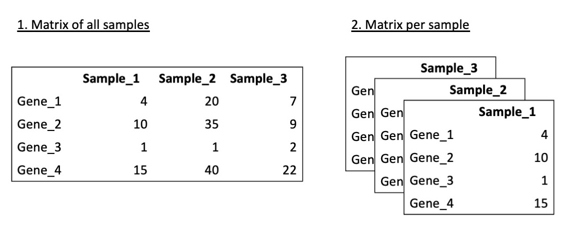
The data may be given as a matrix of features of interest for all samples, or alternatively as a separate file for each sample.
It is important to carefully read the protocols to understand determine how the data has been processed and if is appropriate for your task.
The starting point for a machine learning model is processed RNA-Seq data, in the form of count data. This could be raw count data, or TPM or FPKM pre-processed data.
Dataset Characteristics for supervised learning
Machine learning / AI modelling is a powerful tool in the analysis of RNA-Seq gene expression data. ML techniques are widely used to discover new biomarkers for disease diagnosis and treatment monitoring, and to discover hidden patterns in gene expression that enhance our understanding of the underlying biological pathways. The success of a ML/AI model depends heavily on the input data. Finding an appropriate dataset can be a challenge and the data must be selected carefully as a predictive model trained on the unreliable or inappropriate data will produce unreliable predictions.
There is currently no curated “ML/AI ready” datasets that meet the requirements of machine learning analyses within public functional genomics repositories. It is therefore important to examine a data set carefully to confirm its appropriateness for a supervised machine learning task. The following characteristics of the data should be considered:
| Characteristic | Considerations |
|---|---|
| Quality and Provenance | Assess source of the data, its likely quality and whether it is recognised by the community. Datasets must have sufficient metadata, ideally connected to a domain-specific or community-specific ontology so that the meaning is widely interpretable and comparable between studies. |
| Size | Ensure the data set captures the full complexity of the underlying distribution. If there is significant biological heterogeneity in the sample population, will there be sufficient samples to create independent and representative train, validation and tests sets? Bulk RNA-Seq datasets with only a few samples for each group are unlikely to be sufficient to train a machine learning classifier. |
| Format and Integrity | Machine learning models require data to be machine readable and input in a specific format. Data collected experimentally and data acquired from public repositories will likely need to be reformatted and checked for integrity issues. |
| Technical Noise | RNA-Seq data is likely to contain some technical noise resulting from experimental processes that is unrelated to the underlying biology. This has the potential to bias machine learning algorithms and should be identified and ideally removed. |
| Distribution and Scale | Many machine learning algorithms are sensitive to the distribution and the scale of the input data. RNA-Seq data must be transformed and re-scaled to perform well in a machine learning analysis. |
In the following episodes, we will address each of these issues in turn, working through the collection of a RNA-Seq dataset, reformatting, integrity checking, noise elimination, transformation and rescaling to make the data ready for machine learning. Further information on some of the data considerations in supervised machine learning with biological data can be found in the DOME recommendations.
Key Points
- The two main repositories for sourcing RNA-Seq datasets are ArrayExpress and GEO
- Processed data, in the form of raw counts, or further processed counts data is the starting point for machine learning analysis
- Sourcing and appropriate RNA-Seq dataset and preparing it for a machine learning analysis requires you to consider the dataset quality, size, format, noise content, data distribution and scale
Content from Data Collection: ArrayExpress
Last updated on 2024-05-14 | Edit this page
Overview
Questions
- What format are processed RNA-Seq dataset stored on Array Express?
- How do I search for a dataset that meets my requirements on Array Express?
- Which files do I need to download?
Objectives
- Explain the expected data and file formats for processed RNA-Seq datasets on ArrayExpress
- Demonstrate ability to correctly identify the subset of files required to create a dataset for a simple supervised machine learning task (e.g., binary classification)
- Demonstrate ability to download and save processed RNA-Seq data files from ArrayExpress suitable for a simple supervised machine learning task (e.g., binary classification)
ArrayExpress File Formats
Array Express data sets comprise of four important file types that contain all of the information about an experiment:
| File Type | What It Is |
|---|---|
| Sample and Data Relationship Format (SDRF) | Tab-delimited file containing information about the samples, such as phenotypical information, and factors that may be of interest in a classification task. This file may also contain information about the relationships between the samples, and details of the file names of the raw data fastq for each sample. |
| Investigation Description Format (IDF) | Tab-delimited file containing top level information about the experiment including title, description, submitter contact details and protocols. |
| Raw data files | Sequence data and quality scores, typically stored in FASTQ format. There is however inconsistency - in some data sets, the term raw data refers to processed data in the form of raw counts data, meaning RNA-Seq counts that have not undergone further processing. |
| Processed data files | Processed data which includes raw counts or further processed abundance measures such as TPM and FPKM. The data may be provided as a separate file for each sample, or as a matrix of all samples |
Detailed information about BioStudies file formats is available in the MAGE-TAB Specification document.
Searching for a Dataset on ArrayExpress
We will use ArrayExpress to select an RNA-Seq dataset with a case control design, suitable for constructing a machine learning classification model. Machine learning based analyses generally perform better the larger the sample size, and may perform very poorly and give misleading results with insufficient samples. Given that, we’ll look for a datasets with a relatively large number of samples.
Let’s begin on the ArrayExpress home page.

We’ll apply the following filters to refine the results set, leaving all other filters as the default with no selection:
| Filter | Selection |
|---|---|
| Study type | rna-seq of coding rna |
| Organism | homo sapiens |
| Technology | sequencing assay |
| Assay by Molecule | rna assay |
| Processed Data Available | yes (check box) |
Now use the sort in the top right of the screen to sort the results by “Samples”, in descending order. The results should look similar to this:

Illustrative Dataset: IBD Dataset
In the search results displayed above, the top-ranked dataset is E-MTAB-11349: Whole blood expression profiling of patients with inflammatory bowel diseases in the IBD-Character cohort. We’ll call it the IBD dataset.
The IBD dataset comprises human samples of patients with inflammatory bowel diseases and controls. The ‘Protocols’ section explains the main steps in the generation of the data, from RNA extraction and sample preparation, to sequencing and processing of the raw RNA-Seq data. The nucleic acid sequencing protocol gives details of the sequencing platform used to generate the raw fastq data, and the version of the human genome used in the alignment step to generate the count data. The normalization data transformation protocol gives the tools used to normalise raw counts data for sequence depth and sample composition, in this case normalisation is conducted using the R package DESeq2. DESEq2 contains a range of functions for the transformation and analysis of RNA-Seq data. Let’s look at some of the basic information on this dataset:
| Data Field | Values |
|---|---|
| Sample count | 590 |
| Experimental Design | case control design |
| Experimental factors | Normal, Ulcerative colitis, Crohn’s disease |
The dataset contains two alternative sets of processed data, a matrix of raw counts, and a matrix of processed counts that have been normalised using DESeq2, and filtered to only include transcripts with a mean raw expression read count > 10.
Downloading and Reading into R
Let’s download the SDRF file and the raw counts matrix - these are
the two files that contain the information we will need to build a
machine-learning classification model. In the data files box to the
right-hand side, check the following two files
E-MTAB-11349.sdrf.txt and
ArrayExpress-raw.csv, and save them in a folder called
data in the working directory for your R project. For
consistency, rename ArrayExpress-raw.csv as
E-MTAB-11349.counts.matrix.csv.
For convenience, a copy of the files is also stored on zenodo. You
can run the following code that uses the function
download.file() to download the files and save them
directly into your data directory. (You need to have
created the data directory beforehand).
To get or set a working directory in R getwd function
can be used to return an absolute file path representing the current
working directory of the R process; if not correct setwd
can be used to set the working directory to the desired location.
R
download.file(url = "https://zenodo.org/record/8125141/files/E-MTAB-11349.sdrf.txt",
              destfile = "data/E-MTAB-11349.sdrf.txt")

download.file(url = "https://zenodo.org/record/8125141/files/E-MTAB-11349.counts.matrix.csv",
              destfile = "data/E-MTAB-11349.counts.matrix.csv")
Raw counts matrix
In R studio, open your project workbook and read the raw counts data. Then check the dimensions of the matrix to confirm we have the expected number of samples and transcript IDs.
R
raw.counts.ibd <- read.table(file="data/E-MTAB-11349.counts.matrix.csv",
                             sep=",",
                             header=T,
                             fill=T,
                             check.names=F)

writeLines(sprintf("%i %s", c(dim(raw.counts.ibd)[1], dim(raw.counts.ibd)[2]), c("rows corresponding to transcript IDs", "columns corresponding to samples")))
OUTPUT
22751 rows corresponding to transcript IDs
592 columns corresponding to samplesR
raw.counts.ibd[1:10,1:8]
OUTPUT
            read Sample 1 Sample 2 Sample 3 Sample 4 Sample 5 Sample 6
1   1          *    13961    16595    20722    17696    25703    20848
2   2 ERCC-00002        0        0        0        0        0        0
3   3 ERCC-00003        0        0        0        0        0        0
4   4 ERCC-00004        0        0        0        0        3        0
5   5 ERCC-00009        0        0        0        0        0        0
6   6 ERCC-00012        0        0        0        0        0        0
7   7 ERCC-00013        0        0        0        0        0        0
8   8 ERCC-00014        0        0        0        0        0        0
9   9 ERCC-00016        0        0        0        0        0        0
10 10 ERCC-00017        2        0        0        0        1        0
SDRF File
Now let’s read the sdrf file (a plain text file) into R and check the dimensions of the file.
R
# read in the sdrf file

samp.info.ibd <- read.table(file="data/E-MTAB-11349.sdrf.txt", sep="\t", header=T, fill=T, check.names=F)

sprintf("There are %i rows, corresponding to the samples", dim(samp.info.ibd)[1])
OUTPUT
[1] "There are 590 rows, corresponding to the samples"R
sprintf("There are %i columns, corresponding to the available variables for each sample", dim(samp.info.ibd)[2])
OUTPUT
[1] "There are 32 columns, corresponding to the available variables for each sample"If we view the column names, we can see that the file does indeed contain a set of variables describing both phenotypical and experimental protocol information relating to each sample.
R
colnames(samp.info.ibd)
OUTPUT
 [1] "Source Name"
 [2] "Characteristics[organism]"
 [3] "Characteristics[age]"
 [4] "Unit[time unit]"
 [5] "Term Source REF"
 [6] "Term Accession Number"
 [7] "Characteristics[developmental stage]"
 [8] "Characteristics[sex]"
 [9] "Characteristics[individual]"
[10] "Characteristics[disease]"
[11] "Characteristics[organism part]"
[12] "Material Type"
[13] "Protocol REF"
[14] "Protocol REF"
[15] "Protocol REF"
[16] "Extract Name"
[17] "Material Type"
[18] "Comment[LIBRARY_LAYOUT]"
[19] "Comment[LIBRARY_SELECTION]"
[20] "Comment[LIBRARY_SOURCE]"
[21] "Comment[LIBRARY_STRATEGY]"
[22] "Protocol REF"
[23] "Performer"
[24] "Assay Name"
[25] "Technology Type"
[26] "Protocol REF"
[27] "Derived Array Data File"
[28] "Comment [Derived ArrayExpress FTP file]"
[29] "Protocol REF"
[30] "Derived Array Data File"
[31] "Comment [Derived ArrayExpress FTP file]"
[32] "Factor Value[disease]"
Key Points
- ArrayExpress stores two standard files with information about each experiment: 1. Sample and Data Relationship Format (SDRF) and 2. Investigation Description Format (IDF).
- ArrayExpress provides raw and processed data for RNA-Seq datasets, typically stored as csv, tsv, or txt files.
- The filters on the ArrayExpress website allow you to select and download a dataset that suit your task.
Content from Data Collection: GEO
Last updated on 2024-05-14 | Edit this page
Overview
Questions
- What format are processed RNA-Seq dataset stored on GEO?
- How do I search for a dataset that meets my requirements on GEO?
- How do I use the R package
GEOqueryto download datasets from GEO into R?
Objectives
- Explain the expected data and file formats for processed RNA-Seq datasets on GEO
- Demonstrate ability to correctly identify the subset of files required to create a dataset for a simple supervised machine learning task (e.g., binary classification)
- Demonstrate ability to download and save processed RNA-Seq data files from GEO suitable for a simple supervised machine learning task (e.g., binary classification)
GEO Data Objects
NCBI ‘gene expression omnibus’ , GEO, is one of the largest repositories for functional genomics data. GEO data are stored as individual samples, series of samples and curated datasets. Accession numbers of GEO broadly fall into four categories:
- GSM - GEO Sample. These refer to a single sample.
- GSE - GEO Series. These refer to a list of GEO samples that together form a single experiment.
- GDS - GEO Dataset. These are curated datasets containing summarised information from the underlying GEO samples.
There are many more datasets available as series than there are curated GEO Datasets. For this lesson, we’ll focus on finding a GEO Series as an illustrative dataset.
GEO File Formats
Data for RNA-Seq studies have three components on GEO (similar to microarray studies):
- Metadata
The metadata is equivalent to sample data relationship information provided on ArrayExpress and refers to the descriptive information about the overall study and individual samples. Metadata also contains protocol information and references to the raw and processed data files names for each sample. Metadata is stored in the following standard formats on GEO:
- SOFT (Simple Omnibus Format in Text) is a line-based plain text format
- MINiML is an alternative to SOFT and offers an XML rendering of SOFT
- Series Matrix is a summary text files that include a tab delimited value-matrix table
The raw and processed counts data is typically not included in any of the above files for an RNA-Seq experiement (whereas they may be included with a microarray experiment).
- Processed data files
Processed data (raw counts, noramlised counts) are typically provided in a supplementary file, often a .gz archive of text files. Raw and normalised counts may be provided as separate supplementary files.
- Raw data files
Raw data files provide the original reads and quality scores and are stored in the NIH’s Sequence Read Archive (SRA).
Further information on how RNA-Seq experiments are stored on GEO is given in the submission guidelines on the GEO website.
Searching for a Dataset on GEO
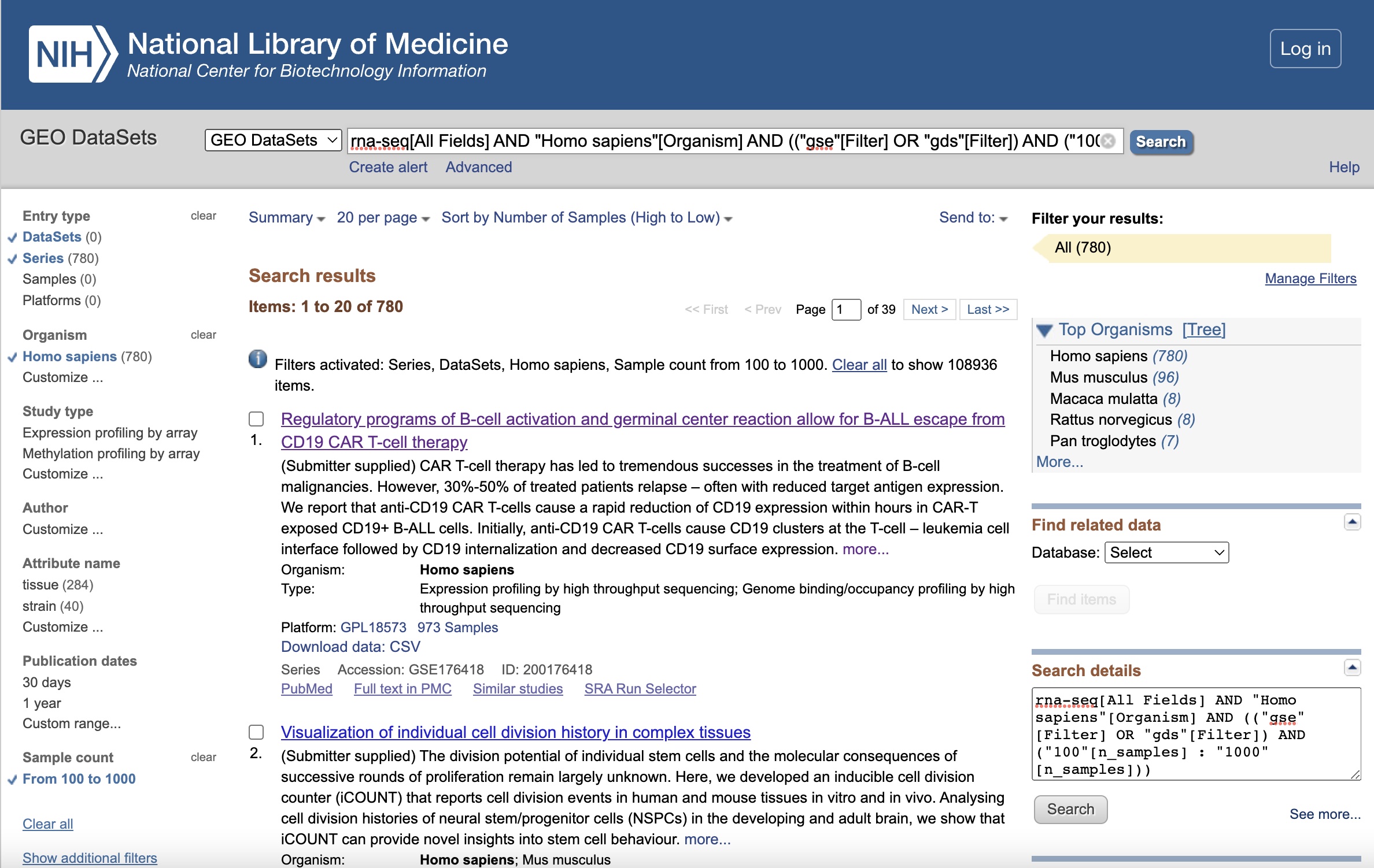
Let’s begin on the GEO home page. GEO provides online search and filter tools. We search by adding “rna-seq” as a keyword in the search box, and then apply the following filters to the subsequent results page, and rank the results by the number of samples in descending order:
| Filter | Selection |
|---|---|
| Keywords. | “rna-seq” |
| Entry type | Series or DataSets |
| Organism | homo sapiens |
| Sample count | From 100 to 1,000 |
The full search string is:
rna-seq[All Fields] AND "Homo sapiens"[Organism] AND (("gse"[Filter] OR "gds"[Filter]) AND ("100"[n_samples] : "1000"[n_samples]))
The filtered results page should looks like this:
Illustrative Dataset: Covid-19 Dataset
The data set GSE212041 relates to the case-control study of neutrophils in Covid-19+ patients named “Longitudinal characterization of circulating neutrophils uncovers phenotypes associated with severity in hospitalized COVID-19 patients” and comprises longitudinal human samples from 306 hospitalized COVID-19+ patients, 78 symptomatic controls, and 8 healthy controls, each at multiple time points, with a total of 781 samples. We’ll call it the Covid-19 dataset. Processed data is provided as raw counts and TPM normalised counts in the Supplementary files.
Let’s look at some of the basic information on this dataset:
| Data Field | Values |
|---|---|
| Sample count | 781 |
| Experimental Design | case control design |
| Experimental factors | COVID+, COVID- symptomatic, healthy |
Downloading and Reading into R
Using GEOquery to download a GEO series as an expression set
The function getGEO() from the GEOquery
library provides a convenient way to download GEO SOFT format data into
R. Here we will download the GEO Series GSE212041. This blog provides
additional information on reading
GEO SOFT files into R
If there is more than one SOFT file for a GEO Series,
getGEO() will return a list of datasets. Let’s download
GSE212041.
R
gse212041 <- GEOquery::getGEO("GSE212041")
OUTPUT
Setting options('download.file.method.GEOquery'='auto')OUTPUT
Setting options('GEOquery.inmemory.gpl'=FALSE)OUTPUT
Found 2 file(s)OUTPUT
GSE212041-GPL18573_series_matrix.txt.gzOUTPUT
GSE212041-GPL24676_series_matrix.txt.gzR
sprintf("Number of files downloaded: %i", length(gse212041))
OUTPUT
[1] "Number of files downloaded: 2"R
writeLines(sprintf("file %i: %i samples", 1:2, c(dim(gse212041[[1]])[2], dim(gse212041[[2]])[2])))
OUTPUT
file 1: 16 samples
file 2: 765 samples
Extracting the Metadata
We’ll extract the metadata for the larger dataset (765 samples) and examine the column names to verify that the file contains the expected metadata about the experiment.
R
samp.info.cov19 <- Biobase::pData(gse212041[[2]])

colnames(samp.info.cov19)
OUTPUT
 [1] "title"                   "geo_accession"
 [3] "status"                  "submission_date"
 [5] "last_update_date"        "type"
 [7] "channel_count"           "source_name_ch1"
 [9] "organism_ch1"            "characteristics_ch1"
[11] "characteristics_ch1.1"   "characteristics_ch1.2"
[13] "characteristics_ch1.3"   "characteristics_ch1.4"
[15] "molecule_ch1"            "extract_protocol_ch1"
[17] "extract_protocol_ch1.1"  "taxid_ch1"
[19] "description"             "description.1"
[21] "data_processing"         "data_processing.1"
[23] "data_processing.2"       "data_processing.3"
[25] "data_processing.4"       "platform_id"
[27] "contact_name"            "contact_email"
[29] "contact_phone"           "contact_laboratory"
[31] "contact_institute"       "contact_address"
[33] "contact_city"            "contact_state"
[35] "contact_zip/postal_code" "contact_country"
[37] "data_row_count"          "instrument_model"
[39] "library_selection"       "library_source"
[41] "library_strategy"        "supplementary_file_1"
[43] "acuity.max:ch1"          "cell type:ch1"
[45] "covid-19 status:ch1"     "patient category:ch1"
[47] "time point:ch1"
Getting the Counts Data
If we use the exprs() function to extract the counts
data from the expression slot of the downloaded dataset, we’ll see that
in this data series, the counts matrix is not there. The expression set
only contains a list of the accession numbers of the samples included in
the expression set, but not the actual count data. (The code below
attempts to view a sample of the data).
R
Biobase::exprs(gse212041[[2]])[,1:10]
OUTPUT
     GSM6507615 GSM6507616 GSM6507617 GSM6507618 GSM6507619 GSM6507620
     GSM6507621 GSM6507622 GSM6507623 GSM6507624
We can verify this by looking at the dimensions of the object in the exprs slot.
R
dim(Biobase::exprs(gse212041[[2]]))
OUTPUT
[1] 0 765To get the counts data, we need to download the Supplementary file
(not downloaded by the getGeo() function). The
GEOquery::getGEOSuppFiles() function enables us to view and
download supplementary files attached to a GEO Series (GSE). This
function doesn’t parse the downloaded files, since the file format may
vary between data series.
Set the ‘fetch_files’ argument to FALSE initially to view the available files.
R
GEOquery::getGEOSuppFiles(GEO = "GSE212041",
                          makeDirectory = FALSE,
                          baseDir = "./data",
                          fetch_files = FALSE,
                          filter_regex = NULL
                          )$fname
OUTPUT
[1] "GSE212041_Neutrophil_RNAseq_Count_Matrix.txt.gz" "GSE212041_Neutrophil_RNAseq_TPM_Matrix.txt.gz"
Challenge 2: Download the supplementary files
Now Download the file to your /data subdirectory, by setting
fetch_files to TRUE and apply a filter_regex
of '*Count_Matrix*' to include the raw counts file only.
Read a sample of the file into R and check the dimensions of the file
correspond to the expected number of samples.
R
GEOquery::getGEOSuppFiles(GEO = "GSE212041",
                          makeDirectory = FALSE,
                          baseDir = "./data",
                          fetch_files = TRUE,
                          filter_regex = '*Count_Matrix*'
                          )

raw.counts.cov19 <- read.table(file="data/GSE212041_Neutrophil_RNAseq_Count_Matrix.txt.gz",
                             sep="\t",
                             header=T,
                             fill=T,
                             check.names=F)

sprintf("%i rows, corresponding to transcript IDs", dim(raw.counts.cov19)[1])
sprintf("%i columns, corresponding to samples", dim(raw.counts.cov19)[2])
OUTPUT
[1] "60640 rows, corresponding to transcript IDs"
[1] "783 columns, corresponding to samples"
R
gse157657 <- GEOquery::getGEO("GSE157657")

samp.info.geotb <- Biobase::pData(gse157657[[1]])

GEOquery::getGEOSuppFiles(GEO = "GSE157657",
                          makeDirectory = FALSE,
                          baseDir = "./data",
                          fetch_files = TRUE,
                          filter_regex = NULL
                          )

raw.counts.geotb <- read.table(file="data/GSE157657_norm.data.txt.gz",
                             sep="\t",
                             header=T,
                             fill=T,
                             check.names=F)

sprintf("%i rows, corresponding to transcript IDs", dim(raw.counts.geotb)[1])
sprintf("%i columns, corresponding to samples", dim(raw.counts.geotb)[2])
OUTPUT
[1] "58735 rows, corresponding to transcript IDs"
[1] "761 columns, corresponding to samples"
Hint: you’ll need to refer back to the GEO website to understand how the data has been processed.
The counts data have been normalised and transformed using a variance
stabilising transformation using the DESeq2 R library.
Key Points
- Similar to ArrayExpress, GEO stores samples information and counts
matrices separately. Sample information is typically stored in
SOFTformat, as well as a.txtfile. - Counts data may be stored as raw counts and some further processed form of counts, typically as supplementary files. Always review the documentation to determine what “processed data” refers to for a particular dataset.
-
GEOqueryprovides a convenient way to download files directly from GEO into R.
Content from Data Readiness: Data Format and Integrity
Last updated on 2024-05-14 | Edit this page
Overview
Questions
- What format do I require my data in to build a supervised machine learning classifier?
- What are the potential data format and data integrity issues I will encounter with RNA-Seq datasets, including those downloaded from public repositories, that I’ll need to address before beginning any analysis?
Objectives
- Describe the format of a dataset required as input to a simple supervised machine learning analysis
- Recall a checklist of common formatting and data integrity issues encountered with sample information (metadata) in RNA-Seq datasets
- Recall a checklist of common formatting and data integrity issues encountered with counts matrix RNA-Seq datasets
- Recall why formatting and data integrity issues present a problem for downstream ML analysis
- Apply the checklist to an unseen dataset downloaded from either the Array Express or GEO platform to identify potential issues
- Construct a reusable R code pipeline implement required changes to a new dataset
Required format for machine learning libraries
Data must be correctly formatted for use in a machine learning / AI pipeline. The garbage in garbage out principle applies; a machine learning model is only as good as the input data. This episode first discusses the kind of data required as input to a machine learing classification model. We’ll then illustrates the process of formatting an RNA-Seq dataset downloaded from a public repository. On the way, we’ll define a checklist of data integrity issues to watch out for.
For a supervised machine learning classification task, we require:
A matrix of values of all of the predictor variables to be included in a machine learning model for each of the samples. Example predictor variables would be gene abundance in the form of read counts. Additional predictor variables may be obtained from the sample information including demographic data (e.g.
sex,age) and clinical and laboratory measures.A vector of values for the target variable that we are trying to predict for each sample. Example target variables for a classification model would be disease state, for example ‘infected with tuburculosis’ compared with ‘healthy control’. The analogy for a regression task would be a continuous variable such as a disease progression or severity score.
We will follow a series of steps to reformat and clean up the sample information and counts matrix file for the IBD dataset collected form ArrayExpress in Episode 2 by applying a checklist of data clean up items. If required, the data can be downloaded again by running this code.
R
download.file(url = "https://zenodo.org/record/8125141/files/E-MTAB-11349.sdrf.txt",
              destfile = "data/E-MTAB-11349.sdrf.txt")

download.file(url = "https://zenodo.org/record/8125141/files/E-MTAB-11349.counts.matrix.csv",
              destfile = "data/E-MTAB-11349.counts.matrix.csv")
We’ll start by reading in the dataset from our data
subfolder.
R
samp.info.ibd <- read.table(file="./data/E-MTAB-11349.sdrf.txt", sep="\t", header=T, fill=T, check.names=F)

raw.counts.ibd <- read.table(file="./data/E-MTAB-11349.counts.matrix.csv", sep="," , header=T, fill=T, check.names=F)
IDB dataset: Sample Information Clean Up
In real RNA-Seq experiments, sample information (metadata) has likely been collected from a range of sources, for example medical records, clinical and laboratory readings and then manually compiled in a matrix format, often a spreadsheet, before being submitted to a public respository. Each of these steps has the potential to introduce errors and inconsistency in the data that must be investigated prior to any downstream machine learning analysis. Whether you are working with sample information received directly from co-workers or downloaded from a public repsository, the following guidelines will help identify and resolve issues that may impact downstream analysis.
Sample Information Readiness Checklist
| Item | Check For… | Rationale |
|---|---|---|
| 1 | Unique identifier matching between counts matrix and sample information | Target variables must be matched to predictor variables for each sample. Target variables are the thing we are trying to predict such as disease state. Predictor variables are the things we are going to predict based on, such as the expression levels of particular genes. |
| 2 | Appropriate target variable present in the data | The sample information needs to contain the target variable you are trying to predict with the machine learning model |
| 3 | Unique variable names, without spaces or special characters | Predictor variables may be drawn from the sample information. ML algorithms require unique variables. Spaces etc. may cause errors with bioinformatics and machine learning libraries used downstream |
| 4 | Machine readable and consistent encoding of categorical variables | Inconsistent spellings between samples will be treated as separate values. Application specific formatting such as colour coding and notes in spreadsheets will be lost when converting to plain text formats. |
| 5 | Numerical class values formatted as a factor (for classification) | Some machine learning algorithms/libraries (e.g. SVM) require classes defined by a number (e.g. -1 and +1 ) |
| 6 | Balance of classes in the target variable (for classification) | Imbalanced datasets may negatively impact results of machine learning algorithms |
We’ll now apply these steps sequentially to the sample information
for the IBD dataset, contained in our variable
samp.info.ibd. First let’s take a look at the data:
R
dplyr::glimpse(samp.info.ibd)
OUTPUT
Rows: 590
Columns: 32
$ `Source Name`                             <chr> "Sample 1", "Sample 2", "Sam…
$ `Characteristics[organism]`               <chr> "Homo sapiens", "Homo sapien…
$ `Characteristics[age]`                    <int> 34, 49, 27, 9, 34, 60, 54, 2…
$ `Unit[time unit]`                         <chr> "year", "year", "year", "yea…
$ `Term Source REF`                         <chr> "EFO", "EFO", "EFO", "EFO", …
$ `Term Accession Number`                   <chr> "UO_0000036", "UO_0000036", …
$ `Characteristics[developmental stage]`    <chr> "adult", "adult", "adult", "…
$ `Characteristics[sex]`                    <chr> "male", "female", "male", "m…
$ `Characteristics[individual]`             <int> 1, 2, 3, 4, 5, 6, 7, 8, 9, 1…
$ `Characteristics[disease]`                <chr> "Crohns disease\tblood\torga…
$ `Characteristics[organism part]`          <chr> "", "blood", "blood", "blood…
$ `Material Type`                           <chr> "", "organism part", "organi…
$ `Protocol REF`                            <chr> "", "P-MTAB-117946", "P-MTAB…
$ `Protocol REF`                            <chr> "", "P-MTAB-117947", "P-MTAB…
$ `Protocol REF`                            <chr> "", "P-MTAB-117948", "P-MTAB…
$ `Extract Name`                            <chr> "", "Sample 2", "Sample 3", …
$ `Material Type`                           <chr> "", "RNA", "RNA", "RNA", "RN…
$ `Comment[LIBRARY_LAYOUT]`                 <chr> "", "PAIRED", "PAIRED", "PAI…
$ `Comment[LIBRARY_SELECTION]`              <chr> "", "other", "other", "other…
$ `Comment[LIBRARY_SOURCE]`                 <chr> "", "TRANSCRIPTOMIC", "TRANS…
$ `Comment[LIBRARY_STRATEGY]`               <chr> "", "Targeted-Capture", "Tar…
$ `Protocol REF`                            <chr> "", "P-MTAB-117950", "P-MTAB…
$ Performer                                 <chr> "", "Wellcome Trust Clinical…
$ `Assay Name`                              <chr> "", "Sample 2", "Sample 3", …
$ `Technology Type`                         <chr> "", "sequencing assay", "seq…
$ `Protocol REF`                            <chr> "", "P-MTAB-117949", "P-MTAB…
$ `Derived Array Data File`                 <chr> "", "ArrayExpress-normalized…
$ `Comment [Derived ArrayExpress FTP file]` <chr> "", "ftp://ftp.ebi.ac.uk/pub…
$ `Protocol REF`                            <chr> "", "P-MTAB-117949", "P-MTAB…
$ `Derived Array Data File`                 <chr> "", "ArrayExpress-raw.csv", …
$ `Comment [Derived ArrayExpress FTP file]` <chr> "", "ftp://ftp.ebi.ac.uk/pub…
$ `Factor Value[disease]` <chr> "", "normal", "normal", "nor…All of the checklist items apply in this case. Let’s go through them…
- Let’s verify that there is a unique identifier that matches between
the sample information and counts matrix, and identify the name of the
column in the sample information. We manually find the names of the
samples in
raw.counts.ibd(the counts matrix), and set to a new variableibd.samp.names. We then write afor loopthat evaluates which columns in the sample information match the sample names. There is one match, the column namedSource Name. Note that there are other columns such asAssay Namein this dataset that contain identifiers for some but not all samples. This is a good illustration of why it is important to check carefully to ensure you have a complete set of unique identifiers.
R
ibd.samp.names <- colnames(raw.counts.ibd)[3:ncol(raw.counts.ibd)]

lst.colnames <- c()
for(i in seq_along(1:ncol(samp.info.ibd))){
  lst.colnames[i] <- all(samp.info.ibd[,i] == ibd.samp.names)
}

sprintf("The unique IDs that match the counts matrix are in column: %s", colnames(samp.info.ibd)[which(lst.colnames)])
OUTPUT
[1] "The unique IDs that match the counts matrix are in column: Source Name"- We next extract this unique identifier along with the condition of
interest, (in this case the
disease), and any other variables that may be potential predictor variables or used to assess confounding factors in the subsequent analysis of the data (in this case patientsexandage). We will use functions from thedplyrpackage, part of thetidyversecollection of packages throughout this episode.
R
samp.info.ibd.sel <- dplyr::select(samp.info.ibd,
                              'Source Name',
                              'Characteristics[age]',
                              'Characteristics[sex]',
                              'Characteristics[disease]'
                              )
- Let’s then rename the variables to something more easy to interpret
for humans, avoiding spaces and special characters. We’ll save these
selected columns to a new variable name
samp.info.ibd.sel.
R
samp.info.ibd.sel <- dplyr::rename(samp.info.ibd.sel,
                          'sampleID' = 'Source Name',
                          'age' = 'Characteristics[age]',
                          'sex' = 'Characteristics[sex]',
                          'condition' = 'Characteristics[disease]'
                          )
- Now check how each of the variables are encoded in our reduced sample information data to identify any errors, data gaps and inconsistent coding of categorical variables. Firstly let’s take a look at the data.
R
dplyr::glimpse(samp.info.ibd.sel)
OUTPUT
Rows: 590
Columns: 4
$ sampleID  <chr> "Sample 1", "Sample 2", "Sample 3", "Sample 4", "Sample 5", …
$ age       <int> 34, 49, 27, 9, 34, 60, 54, 24, 39, 41, 38, 46, 7, 46, 21, 35…
$ sex       <chr> "male", "female", "male", "male", "female", "female", "femal…
$ condition <chr> "Crohns disease\tblood\torganism part\tP-MTAB-117946\tP-MTAB…- There is clearly an issue with the coding of the
conditionCrohn’s disease. We’ll fix that first, and then check the consistency of the coding of categorical variablessexandcondition.
R
samp.info.ibd.sel$condition[agrep("Crohns", samp.info.ibd.sel$condition)] <- "crohns_disease"

unique(c(samp.info.ibd.sel$sex, samp.info.ibd.sel$condition))
OUTPUT
[1] "male"               "female"             "crohns_disease"
[4] "normal" "ulcerative colitis"- Both
sexandconditionare consistently encoded over all samples. We should however remove the spaces in the values forsampleIDand for theconditionvalue ulcerative colitis. Note: since we are changing our unique identifier, we’ll need to make the same update later in the counts matrix.
Before we do this, since we’ll be using the pipe operator from the tidyverse libraries, we will to define the pipe operator from the magrittr package in the environment.
R
`%>%` <- magrittr::`%>%`

samp.info.ibd.sel <- samp.info.ibd.sel %>%
                        dplyr::mutate(sampleID = gsub(" ", "_", sampleID),
                                      condition = gsub(" ", "_", condition))
- As some machine learning classification algorithms such as support
vector machines require a numerical input for each class, we’ll add in a
new numerical column to represent our target variable called
classwhere all patients denoted asnormalare given the value -1, and all patients denoted as eithercrohns_diseaseorulcerative_colitisare given the vale +1. We’ll also now convert the type of categorical columns to factors as this is preferred by downstream libraries used for data normalisation such as DESeq2.
R
samp.info.ibd.sel <- samp.info.ibd.sel %>%
                        dplyr::mutate(class = dplyr::if_else(condition == 'normal', -1, 1))
R
samp.info.ibd.sel[c('sex', 'condition', 'class')] <- lapply(samp.info.ibd.sel[c('sex', 'condition', 'class')], factor)
- Finally, let’s check the distribution of the classes by creating a
tablefrom theclasscolumn.
R
table(samp.info.ibd.sel$class)
OUTPUT
 -1   1
267 323
The two classes are approximately equally represented, so let’s check everything one last time.
R
dplyr::glimpse(samp.info.ibd.sel)
OUTPUT
Rows: 590
Columns: 5
$ sampleID  <chr> "Sample_1", "Sample_2", "Sample_3", "Sample_4", "Sample_5", …
$ age       <int> 34, 49, 27, 9, 34, 60, 54, 24, 39, 41, 38, 46, 7, 46, 21, 35…
$ sex       <fct> male, female, male, male, female, female, female, male, male…
$ condition <fct> crohns_disease, normal, normal, normal, normal, ulcerative_c…
$ class     <fct> 1, -1, -1, -1, -1, 1, 1, -1, 1, 1, -1, 1, -1, -1, -1, 1, -1,…
And save the output as a file.
R
write.table(samp.info.ibd.sel, file="./data/ibd.sample.info.txt", sep = '\t', quote = FALSE, row.names = TRUE)
IDB dataset: Counts Matrix Clean Up
Count Matrix Readiness Checklist
| Item | Check For… | Rationale |
|---|---|---|
| 1 | Extraneous information that you don’t want to include as a predictor variable | Blank rows, alternative gene/ transcript IDs and metadata about the genes/transcripts will be treated as a predictor variable unless you explicitly remove them |
| 2 | Unique variable names, without spaces or special characters | ML algorithms require unique variables. Spaces etc. may cause errors with bioinformatics and ml libraries used downstream (and they must match the sample information) |
| 3 | Duplicate data | Duplicate variables may bias results of analysis and should be removed unless intentional |
| 4 | Missing values | Missing values may cause errors and bias results. Missing values must be identified and appropriate treatment determined (e.g. drop vs impute) |
- Take a look at a sample of columns and rows to see what the downloaded file looks like
R
raw.counts.ibd[1:10,1:8]
OUTPUT
            read Sample 1 Sample 2 Sample 3 Sample 4 Sample 5 Sample 6
1   1          *    13961    16595    20722    17696    25703    20848
2   2 ERCC-00002        0        0        0        0        0        0
3   3 ERCC-00003        0        0        0        0        0        0
4   4 ERCC-00004        0        0        0        0        3        0
5   5 ERCC-00009        0        0        0        0        0        0
6   6 ERCC-00012        0        0        0        0        0        0
7   7 ERCC-00013        0        0        0        0        0        0
8   8 ERCC-00014        0        0        0        0        0        0
9   9 ERCC-00016        0        0        0        0        0        0
10 10 ERCC-00017 2 0 0 0 1 0- Remove the first row, which is in this case totals of counts for each sample
- Remove the first columns, which just numbers the transcript IDs
- Move the column named
readthat contains to the transcript IDs to the row names
R
counts.mat.ibd <- raw.counts.ibd[-1,-1]

rownames(counts.mat.ibd) <- NULL

counts.mat.ibd <-  counts.mat.ibd %>% tibble::column_to_rownames('read')

counts.mat.ibd[1:10,1:6]
OUTPUT
           Sample 1 Sample 2 Sample 3 Sample 4 Sample 5 Sample 6
ERCC-00002        0        0        0        0        0        0
ERCC-00003        0        0        0        0        0        0
ERCC-00004        0        0        0        0        3        0
ERCC-00009        0        0        0        0        0        0
ERCC-00012        0        0        0        0        0        0
ERCC-00013        0        0        0        0        0        0
ERCC-00014        0        0        0        0        0        0
ERCC-00016        0        0        0        0        0        0
ERCC-00017        2        0        0        0        1        0
ERCC-00019 0 0 0 0 0 0- Let’s check for duplicate sampleIDs and transcript IDs. Provided
there are no duplicate row or column names, the following should return
interger(0).
R
which(duplicated(rownames(counts.mat.ibd)))
OUTPUT
integer(0)R
which(duplicated(colnames(counts.mat.ibd)))
OUTPUT
integer(0)- We’ll double check the sampleIDs match the sample information file.
R
if(!identical(colnames(counts.mat.ibd), samp.info.ibd.sel$sampleID)){stop()}
ERROR
Error in eval(expr, envir, enclos): We renamed the samples in the sample information to remove spaces, so we need to do the same here.
R
colnames(counts.mat.ibd) <- gsub(x = colnames(counts.mat.ibd), pattern = "\ ", replacement = "_")
- Finally, we’ll check that there are no missing values in the counts
matrix. Note, there will be many zeros, but we are ensuring that there
are no
NAvalues or black records. The following should returnFALSE.
R
allMissValues <- function(x){all(is.na(x) | x == "")}

allMissValues(counts.mat.ibd)
OUTPUT
[1] FALSETake a final look at the cleaned up matrix.
R
counts.mat.ibd[1:10,1:6]
OUTPUT
           Sample_1 Sample_2 Sample_3 Sample_4 Sample_5 Sample_6
ERCC-00002        0        0        0        0        0        0
ERCC-00003        0        0        0        0        0        0
ERCC-00004        0        0        0        0        3        0
ERCC-00009        0        0        0        0        0        0
ERCC-00012        0        0        0        0        0        0
ERCC-00013        0        0        0        0        0        0
ERCC-00014        0        0        0        0        0        0
ERCC-00016        0        0        0        0        0        0
ERCC-00017        2        0        0        0        1        0
ERCC-00019        0        0        0        0        0        0
R
sprintf("There are %i rows, corresponding to the transcript IDs", dim(counts.mat.ibd)[1])
OUTPUT
[1] "There are 22750 rows, corresponding to the transcript IDs"R
sprintf("There are %i columns, corresponding to the samples", dim(counts.mat.ibd)[2])
OUTPUT
[1] "There are 590 columns, corresponding to the samples"And save the output as a file.
R
write.table(counts.mat.ibd, file="./data/counts.mat.ibd.txt", sep = '\t', quote = FALSE, row.names = TRUE)
Document your reformatting steps
It is crucial that you document your data reformatting so that it is reproducible by other researchers. Create a project folder for your data processing and include:
- Raw input data files collected from ArrayExpress, GEO or similar
- The output counts matrix and target variable vector, stored in a common format such at .txt format
- The full R scripts used to perform all the data clean up steps. Store the script with the input and output data.
- A readme file that explains the steps taken, and how to run the script on the inputs to generate the outputs. This should also include details of all software versions used (e.g. R version, RStudio or Jupyter Notebooks version, and the versions of any code libraries used)
The TB Dataset: Another Example
Discussion
Take a look at The
Tuburculosis (TB) Dataset - E-MTAB-6845. You can download the sdrf
file from zenodo and save it to your data directory by
running the following code.
R
download.file(url = "https://zenodo.org/record/8125141/files/E-MTAB-6845.sdrf.txt",
              destfile = "data/E-MTAB-6845.sdrf.txt")
Read the sdrf file into R and take a look at the data. Make a list of the potential issues with this data based on the checklist above? What steps would need to be taken to get them ready to train a machine learning classifier?
As a help, the code to read the file in from your data directory is:
R
samp.info.tb <- read.table(file="./data/E-MTAB-6845.sdrf.txt", sep="\t", header=T, fill=T, check.names=F)
Challenge Extension
Can you correctly reorder the following code snippets to create a
pipeline to reformat the data in line with the sample information
checklist? Use the
Characteristics[progressor status (median follow-up 1.9 years)]
as the target variable.
R
dplyr::rename(
  'sampleID' = 'Comment[sample id]',
  'prog_status' = 'Factor Value[progressor status (median follow-up 1.9 years)]') %>%

dplyr::select(
            'Comment[sample id]',
            'Factor Value[progressor status (median follow-up 1.9 years)]')  %>%


dplyr::mutate(prog_status = factor(prog_status, levels = c("non_progressor","tb_progressor")),
             class = factor(class, levels = c(-1, 1))) %>%

dplyr::mutate(prog_status = dplyr::recode(prog_status,
              "non-progressor" = "non_progressor",
              "TB progressor" = "tb_progressor"),
              class = dplyr::if_else(prog_status == 'non_progressor', -1, 1)
              ) %>%

dplyr::distinct() %>%

samp.info.tb %>%

dplyr::glimpse()
R
samp.info.tb %>%

      dplyr::select(
            'Comment[sample id]',
            'Factor Value[progressor status (median follow-up 1.9 years)]')  %>%             # select columns

      dplyr::rename(
        'sampleID' = 'Comment[sample id]',
        'prog_status' = 'Factor Value[progressor status (median follow-up 1.9 years)]') %>%  # rename them

      dplyr::distinct() %>%                                                                  # remove duplicate rows

      dplyr::mutate(prog_status = dplyr::recode(prog_status,                                 # recode target variable
                    "non-progressor" = "non_progressor",
                    "TB progressor" = "tb_progressor"),
                    class = dplyr::if_else(prog_status == 'non_progressor', -1, 1)                 # create numerical class
                    ) %>%

       dplyr::mutate(prog_status = factor(prog_status, levels = c("non_progressor","tb_progressor")),
                     class = factor(class, levels = c(-1, 1))) %>%                          # set variables to factors

       dplyr::glimpse()                                                                     # view output
OUTPUT
Rows: 360
Columns: 3
$ sampleID    <chr> "PR123_S19", "PR096_S13", "PR146_S14", "PR158_S12", "PR095…
$ prog_status <fct> non_progressor, non_progressor, non_progressor, non_progre…
$ class       <fct> -1, -1, -1, -1, -1, -1, -1, -1, -1, -1, -1, -1, -1, -1, -1…
Key Points
- Machine learning algorithms require specific data input formats, and for data to be consistently formatted across variables and samples. A classification task for example requires a matrix of the value of each input variable for each sample, and the class label for each sample.
- Clinical sample information is often messy, with inconsistent formatting as a result of how it is collected. This applies to data downloaded from public repositories.
- You must carefully check all data for formatting and data integrity issues that may negatively impact your downstream ml analysis.
- Document your data reformatting and store the code pipeline used along with the raw and reformatted data to ensure your procedure is reproducible
Content from Data Readiness: Technical Noise
Last updated on 2024-05-14 | Edit this page
Overview
Questions
- How do technical artefacts in RNA-Seq data impact machine learning algorithms?
- How can technical artefacts such as low count genes and outlier read counts be effectively removed from RNA-Seq data prior to analysis?
Objectives
- Describe two important sources of technical noise in RNA-Seq data - genes with very low read counts and genes with influential outlier read counts - and recall why these exist in raw datasets
- Demonstrate how to remove these noise elements from RNA-Seq count data to further improve machine learning readiness using standard R libraries
Technical Artefacts in RNA-Seq Data
Machine learning classification algorithms are highly sensitive to any feature data characteristic that differs between experimental groups, and will exploit these differences when training a model. Given this, it is important to make sure that data input into a machine learning model reflects true biological signal, and not technical artefacts or noise that stems from the experimental process used to generate the data. In simple terms, we need to remove things are aren’t “real biological information”.
There are two important sources of noise inherent in RNA-Seq data that may negatively impact machine learning modelling performance, namely low read counts, and influential outlier read counts.
Low read counts
Genes with consistently low read count values across all samples in a dataset may be technical or biological stochastic artefacts such as the detection of a transcript from a gene that is not uniformly active in a heterogeneous cell population or as the result of a transcriptional error. Below some threshold, differences in counts between the conditions of interest for a given gene are unlikely to be representative of true biological differences between the groups. Filtering out low count genes has been show to increase the classification performance of machine learning classifiers, and to increase the stability of the set of genes selected by a machine learning algorithm in the context of selecting relevant genes.
Investigating Low Counts
We’ll briefly investigate the distribution of read counts in the IBD dataset to illustrate this point. Import the cleaned up counts matrix and sample information text files that we prepared in Episode 4. If you didn’t manage to save them, you can download them directly using the following code.
R
download.file(url = "https://zenodo.org/record/8125141/files/ibd.sample.info.txt",
              destfile = "data/ibd.sample.info.txt")

download.file(url = "https://zenodo.org/record/8125141/files/counts.mat.ibd.txt",
              destfile = "data/counts.mat.ibd.txt")
And now read the files into R…
R
# suppressPackageStartupMessages(library(dplyr, quietly = TRUE))
# suppressPackageStartupMessages(library(ggplot2, quietly = TRUE))
# suppressPackageStartupMessages(library(tibble, quietly = TRUE))
R
samp.info.ibd.sel <- read.table(file="./data/ibd.sample.info.txt", sep="\t", header=T, fill=T, check.names=F)

counts.mat.ibd <- read.table(file="./data/counts.mat.ibd.txt", sep='\t', header=T, fill=T, check.names=F)
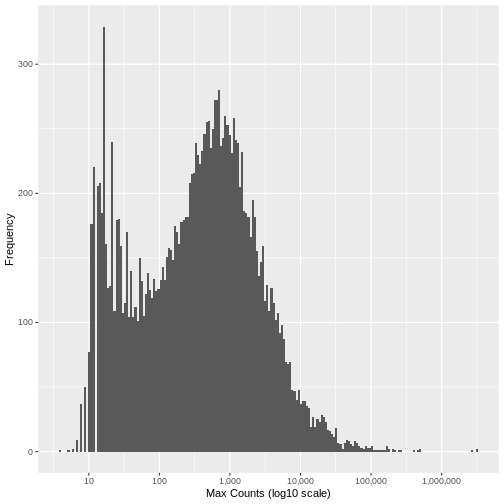
Run the following code to view the histogram giving the frequency of the maximum count for each gene in the sample (plotted on a log10 scale). You’ll see in the resulting plot that over 800 genes have no counts for any gene (i.e., maximum = 0), and that there are hundreds of genes where the maximum count for the gene across all samples is below 10. For comparison, the median of these maximum counts across all genes is around 250. These low count genes are likely to represent technical noise.
A simple filtering approach is to remove all genes where the maximum read count for that gene over all samples is below a given threshold. The next step is to determine what this threshold should be.
R
`%>%` <- magrittr::`%>%`

data.frame(max_count = apply(counts.mat.ibd, 1, max, na.rm=TRUE)) %>%
  ggplot2::ggplot(ggplot2::aes(x = max_count)) +
    ggplot2::geom_histogram(bins = 200) +
    ggplot2::xlab("Max Counts (log10 scale)") +
    ggplot2::ylab("Frequency") +
    ggplot2::scale_x_log10(n.breaks = 6, labels = scales::comma)
WARNING
Warning: Transformation introduced infinite values in continuous x-axisWARNING
Warning: Removed 10 rows containing non-finite values (`stat_bin()`).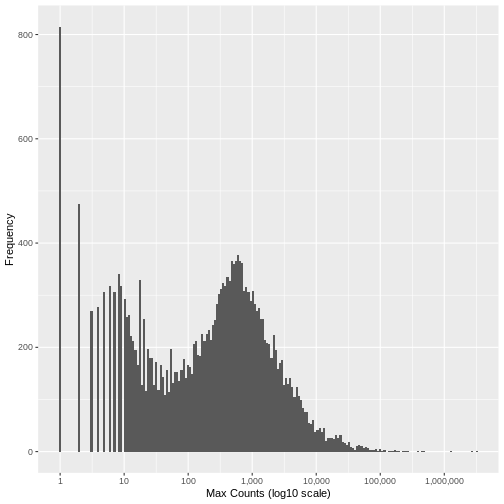
There is no right answer. However, looking at the histogram, you can see an approximately symmetrical distribution centred around a value between 100 and 1,000 (approximately 250), and a second distirbution of low count genes in the range 1-20. From this, we could estimate that the cut off for low count genes will be approximately in the range 10-20.
Read Count Normalisation
In order to be able to compare read counts between samples, we must
first adjust (‘normalise’) the counts to control for differences in
sequence depth and sample composition between samples. To achieve this,
we run the following code that will normalise the counts matrix using
the median-of-ratios method implemented in the R package
DESeq2. For more information on the rationale for scaling
RNA-Seq counts and a comparison of the different metrics used see RDMBites | RNAseq
expression data.
R
# convert the condition variable to a factor as required by DESeq2
samp.info.ibd.sel[c('condition')] <- lapply(samp.info.ibd.sel[c('condition')], factor)

# create DESeq Data Set object from the raw counts (converted to a matrix), with condition as the factor of interest
dds.ibd <- DESeq2::DESeqDataSetFromMatrix(
    countData = as.matrix(counts.mat.ibd),
    colData = data.frame(samp.info.ibd.sel, row.names = 'sampleID'),
    design = ~ condition)
WARNING
Warning: replacing previous import 'S4Arrays::makeNindexFromArrayViewport' by
'DelayedArray::makeNindexFromArrayViewport' when loading 'SummarizedExperiment'
R
# calculate the normalised count values using the median-of-ratios method
dds.ibd <- dds.ibd %>% DESeq2::estimateSizeFactors()

# extract the normalised counts
counts.ibd.norm <- DESeq2::counts(dds.ibd, normalized = TRUE)
Setting a Low Counts Threshold
There are a number of methodologies to calculate the appropriate
threshold. One widely used approach calculates the threshold that
maximises the similarity between the samples, calculating the mean
pairwise Jaccard index over all samples in each conditionn of interest,
and setting the threshold that maximises this value. The motivation for
this measure is that true biological signal will be consistent between
samples in the same condition, however low count noise will be randomly
distributed. By maximising the similarity between samples in the same
class, the threshold is likely to be set above the background noise
level. The code for this filter is implemented in the R package
HTSFilter and the methodology, along with details of
alternative approaches, is described in detail by Rau et al., 2013.
Calculating the Jaccard index between all pairs of samples in a dataset does not however scale well with the dimensionality of the data. Here we use an alternative approach that achieves a very similar result using the Multiset Jaccard index, which is faster to compute. Don’t worry too much about the code, the main point is that we find a filter threshold, and filter out all the genes where the max count value is below the threshold, on the basis that these are likely technical noise. Run the code to plot the Multiset Jaccard Index for a series of values for the filter threshold.
R
# For the purpose of illustration, and to shorten the run time, we sample 5,000 genes from the counts matrix.

set.seed(10)

counts.ibd.norm.samp <- counts.ibd.norm[sample(nrow(counts.ibd.norm), size = 5000, replace = FALSE),]

# create vector of the class labels
condition <- samp.info.ibd.sel$condition

# create a sequence of thresholds to test
t.seq <- seq(1, 25, by = 1)

# Function to calculate the Multiset Jaccard Index' over all samples
Jaccard = function(mat){
  row.sums = rowSums(mat)
  inter = sum(row.sums == ncol(mat))
  union = sum(row.sums > 0)
  return(inter/union)
}

# Calculate vector of the minimum Multiset Jaccard Index over the three classes, for each value of t

ms.jac = sapply(t.seq, function(t){
  filt.counts = counts.ibd.norm.samp >=t
  group.jac = sapply(unique(condition), function(cond){
    Jaccard(filt.counts[,condition==cond])
  })
  return(min(group.jac))
})


# plot the threshold value against the value of the Multiset Jaccard index to visualise

ggplot2::ggplot(data=data.frame(t = t.seq, jacc = ms.jac)) +
            ggplot2::geom_line(ggplot2::aes(x=t, y=jacc)) +
            ggplot2::geom_hline(yintercept = max(ms.jac), lty=2,col='gray') +
            ggplot2::geom_point(ggplot2::aes(x=which.max(ms.jac), y=max(ms.jac)), col="red", cex=6, pch=1) +
            ggplot2::xlab("Low Count Threshold") +
            ggplot2::ylab("Multiset Jaccard Index")
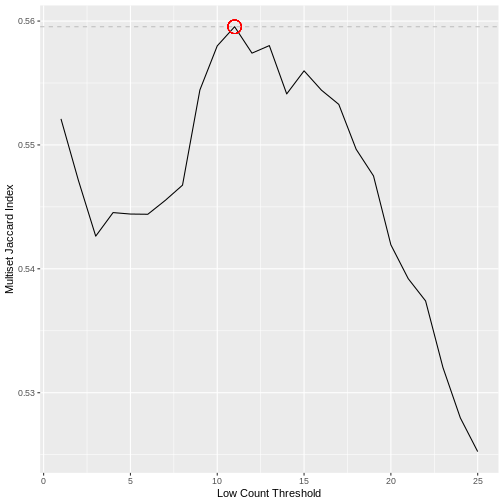
The threshold value is given by the following code, which should return a value close to 10 for this dataset.
R
(t.hold <- which.max(ms.jac))
OUTPUT
[1] 11Filtering Low Counts
Having determined a threshold, we then filter the raw counts matrix on the rows (genes) that meet the threshold criterion based on the normalised counts. As you can see, around 4,000 genes are removed from the dataset, which is approximately 20% of the genes. These genes are unlikely to contain biologically meaningful information but they might easily bias a machine learning classifier.
R
counts.mat.ibd.filtered <- counts.mat.ibd[which(apply(counts.ibd.norm, 1, function(x){sum(x > t.hold) >= 1})),]

sprintf("Genes filtered: %s; Genes remaining: %s", nrow(counts.mat.ibd)-nrow(counts.mat.ibd.filtered), nrow(counts.mat.ibd.filtered))
OUTPUT
[1] "Genes filtered: 3712; Genes remaining: 19038"Outlier Reading Counts
A second source of technical noise is outlier read counts. Relatively high read counts occurring in only a very small number of samples relative to the size of each patient group are unlikely to be representative of the general population and a result of biological heterogeneity and technical effects. These very large count values may bias machine learning algorithms if they help to discriminate between examples in a training set, leading to model overfitting. Such influential outliers may be the result of natural variation between individuals or they may have been introduced during sample preparation. cDNA libraries require PCR amplification prior to sequencing to achieve sufficient sequence depth. This clonal amplification by PCR is stochastic in nature; different fragments may be amplified with different probabilities. This leaves the possibility of outlier read counts having resulted from bias introduced by amplification, rather than biological differences between samples. The presence of these outlier read counts for a particular gene may therefore inflate the observed association between a particular gene and the condition of interest.
Run the following code to view the top 10 values of read counts in the raw counts matrix. Compare this with the histogram above, and the mean read count. The largest read count values range from 2MM to over 3MM counts for a gene in a particular sample. These require investigation!
R
tail(sort(as.matrix(counts.mat.ibd)),10)
OUTPUT
 [1] 2037946 2038514 2043983 2133125 2238093 2269033 2341479 2683585 3188911
[10] 3191428
R
sprintf("The mean read count value: %f", mean(as.matrix(counts.mat.ibd)))
OUTPUT
[1] "The mean read count value: 506.731355"Outlier Read Count Filtering
As with low counts, multiple methods exist to identify influential
outlier read counts. A summary is provided by Parkinson et al..
Here we adopt an approach that is built into the R package
DESeq2 that identifies potential influential outiers based
on their Cooks distance.
Run the following code to create DESeq Data Set object from the filtered raw counts matrix, with condition as the experimental factor of interest.
R
dds.ibd.filt <- DESeq2::DESeqDataSetFromMatrix(
    countData = as.matrix(counts.mat.ibd.filtered),
    colData = data.frame(samp.info.ibd.sel, row.names = 'sampleID'),
    design = ~ condition)
Run DESeq2 differential expression analysis, which
automatically calculates the Cook’s distances for every read count. This
may take a few minutes to run.
R
deseq.ibd <- DESeq2::DESeq(dds.ibd.filt)
OUTPUT
estimating size factorsOUTPUT
estimating dispersionsOUTPUT
gene-wise dispersion estimatesOUTPUT
mean-dispersion relationshipOUTPUT
final dispersion estimatesOUTPUT
fitting model and testingOUTPUT
-- replacing outliers and refitting for 1559 genes
-- DESeq argument 'minReplicatesForReplace' = 7
-- original counts are preserved in counts(dds)
OUTPUT
estimating dispersionsOUTPUT
fitting model and testingR
cooks.mat <- SummarizedExperiment::assays(deseq.ibd)[["cooks"]]
We now calculate the cooks outlier threshold by computing the expected F-distribution for the number of samples in the dataset.
R
cooks.quantile <- 0.95
m <- ncol(deseq.ibd)     # number of samples
p <- 3                   # number of model parameters (in the three condition case)

h.threshold <- stats::qf(cooks.quantile, p, m - p)
Filter the counts matrix to eliminate all genes where the cooks distance is over the outlier threshold. Here you can see that a further ~1,800 genes are filtered out based on having outlier read count values for at least one sample.
R
counts.mat.ibd.ol.filtered <-  counts.mat.ibd.filtered[which(apply(cooks.mat, 1, function(x){(max(x) < h.threshold) >= 1})),]

sprintf("Genes filtered: %s; Genes remaining: %s", nrow(counts.mat.ibd.filtered)-nrow(counts.mat.ibd.ol.filtered), nrow(counts.mat.ibd.ol.filtered))
OUTPUT
[1] "Genes filtered: 1776; Genes remaining: 17262"Run the same plot as above, and we can see that the genes with very low maximum counts over all samples have been removed. Note that here we are looking at the raw unnormalised counts, so not all maximum counts are below 11, as the filter was applied to the normailsed counts.
R
data.frame(max_count = apply(counts.mat.ibd.ol.filtered, 1, max, na.rm=TRUE)) %>%
  ggplot2::ggplot(ggplot2::aes(x = max_count)) +
    ggplot2::geom_histogram(bins = 200) +
    ggplot2::xlab("Max Counts (log10 scale)") +
    ggplot2::ylab("Frequency") +
    ggplot2::scale_x_log10(n.breaks = 6, labels = scales::comma)
Now save the output as a file that we will use in the next episode.
R
write.table(counts.mat.ibd.ol.filtered, file="./data/counts.mat.ibd.ol.filtered.txt", sep = '\t', quote = FALSE, row.names = TRUE)
Key Points
- RNA-Seq read counts contain two main sources of technical ‘noise’ that are unlikely to represent true biological information, and may be artefacts from experimental processes required to generate the data: Low read counts and influential outlier read counts.
- Filtering out low count and influential outlier genes removes potentially biasing variables without negatively impacting the performance of downstream machine learning analysis. Gene filtering is therefore an important step in preparing an RNA-Seq dataset to be machine learning ready.
- Multiple approaches exist to identify the specific genes with uninformative low count and influential outlier read counts in RNA-Seq data, however they all aim to find the boundary between true biological signal and technical and biological artefacts.
Content from Data Readiness: Distribution and Scale
Last updated on 2024-05-14 | Edit this page
Overview
Questions
- Do I need to transform or rescale RNA-Seq data before inputting into a machine learning algorithm?
- What are the most appropriate transformations and how do these depend on the particular machine learning algorithm being employed?
Objectives
- Describe the main characteristics of the distribution of RNA-Seq count data and how this impacts the performance of machine learning algorithms
- Recall the main types of data transformation commonly applied to RNA-Seq count data to account for skewedness and heteroskedasticity
- Demonstrate how to apply these transformations in R
- Recall the two types of data rescaling commonly applied prior to machine learning analysis, and which is most appropriate for a range of common algorithms
RNA-Seq Counts Data: A Skewed Distribution
RNA-Seq count data has an approximately negative binomial distribution. Even after filtering out low count genes, the distribution of count data is heavily skewed towards low counts. Counts data is also heteroskedastic, which means the variance depends on the mean. These two properties negatively impact the performance of some machine learning models, in particular Regression based models. Let’s examine these properties in our dataset.
To begin, import the filtered counts matrix and sample information text files that we prepared in Episodes 4 and 5. If you didn’t manage to save it, you can download it directly with the following code.
R
download.file(url = "https://zenodo.org/record/8125141/files/ibd.sample.info.txt",
              destfile = "data/ibd.sample.info.txt")

download.file(url = "https://zenodo.org/record/8125141/files/counts.mat.ibd.ol.filtered.txt",
              destfile = "data/counts.mat.ibd.ol.filtered.txt")
And now read the files into R…
R
# suppressPackageStartupMessages(library(dplyr, quietly = TRUE))
# suppressPackageStartupMessages(library(ggplot2, quietly = TRUE))
# suppressPackageStartupMessages(library(tibble, quietly = TRUE))
R
samp.info.ibd.sel <- read.table(file="./data/ibd.sample.info.txt", sep="\t", header=T, fill=T, check.names=F)

counts.mat.ibd.ol.filtered <- read.table(file="./data/counts.mat.ibd.ol.filtered.txt", sep='\t', header=T, fill=T, check.names=F)
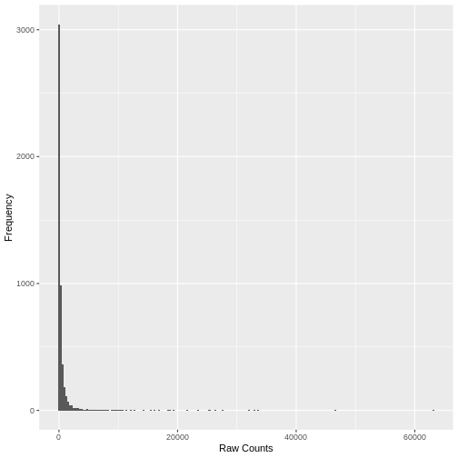
A simple histogram of the raw counts data illustrates the skewed nature of the distribution. Here we plot a random sample of just 5,000 counts to illustrate the point.
R
set.seed(seed = 30)

`%>%` <- magrittr::`%>%`

counts.mat.ibd.ol.filtered %>%
  tibble::rownames_to_column("geneID")  %>%
  reshape2::melt(id.vars = 'geneID', value.name='count', variable.name=c('sampleID')) %>%
  .[sample(nrow(.), size = 5000, replace = FALSE),] %>%
  ggplot2::ggplot(ggplot2::aes(x = count)) +
    ggplot2::geom_histogram(bins = 200) +
    ggplot2::xlab("Raw Counts") +
    ggplot2::ylab("Frequency")
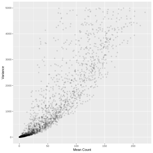
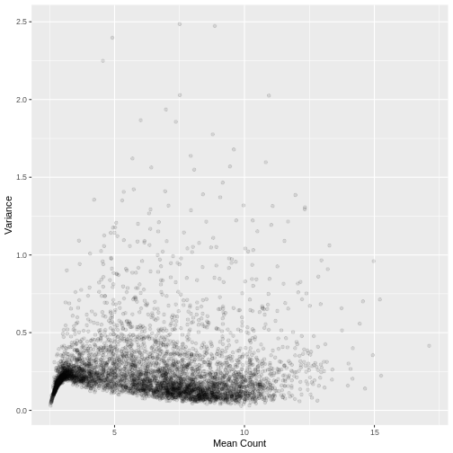
A plot of the mean count against the variance of the counts for a random sample of 5,000 genes (to reduce compute time) illustrates the clear mean variance relationship in the data. The variance is increasing as the mean count increases.
R
counts.mat.ibd.ol.filtered %>%
  .[sample(nrow(.), size = 5000, replace = FALSE),] %>%
  data.frame(row.mean = apply(., 1, mean),
           row.var = apply(., 1, var)) %>%
  dplyr::filter(row.var < 5000) %>%
  ggplot2::ggplot(ggplot2::aes(x=row.mean, y=(row.var))) +
    ggplot2::geom_point(alpha=0.1) +
    ggplot2::xlab("Mean Count") +
    ggplot2::ylab("Variance")
Variance Stabilising and rlog Transformation
A number of standard transformations exist to change the distribution
of RNA-Seq counts to reduce the mean variance relationship, and make the
distribution more ‘normal’ (Gaussian). Two such transformations are the
variance stabilising transformation (vst) and the
rlog transformation available in the DESeq2 R
package. Both transformations take raw counts data as input, and perform
the normalisation step before the transformation.
The vst transformation is faster to run and more
suitable for datasets with a large sample size. Let’s conduct the
vst transformation on our filtered counts data. This may
take a few minutes to run on our dataset.
R
# convert the condition variable to a factor as required by DESeq2
samp.info.ibd.sel[c('condition')] <- lapply(samp.info.ibd.sel[c('condition')], factor)

# create DESeq Data Set object from the raw counts, with condition as the factor of interest
dds.ibd.filt.ol <- DESeq2::DESeqDataSetFromMatrix(
  countData = as.matrix(counts.mat.ibd.ol.filtered),
  colData = data.frame(samp.info.ibd.sel, row.names = 'sampleID'),
  design = ~ condition)
WARNING
Warning: replacing previous import 'S4Arrays::makeNindexFromArrayViewport' by
'DelayedArray::makeNindexFromArrayViewport' when loading 'SummarizedExperiment'
R
# calculate the vst count values and extract the counts matrix using the assay() function
counts.mat.ibd.vst <- DESeq2::varianceStabilizingTransformation(dds.ibd.filt.ol, blind=FALSE) %>%
  SummarizedExperiment::assay()
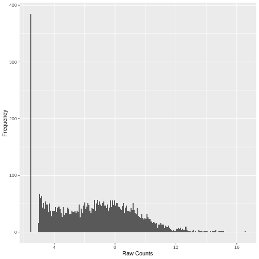
Plotting the data again, we can see the difference in the distribution of the data following transformation. Although there is still a large number of count values equal to zero, the distribution of vst transformed counts is far less heavily skewed than the original. The dependence of the variance on the mean has essentially been eliminated.
R
set.seed(seed = 30)

counts.mat.ibd.vst %>%
  as.data.frame() %>%
  tibble::rownames_to_column("geneID")  %>%
  reshape2::melt(id.vars = 'geneID', value.name='count', variable.name=c('sampleID')) %>%
  .[sample(nrow(.), size = 5000, replace = FALSE),] %>%
  ggplot2::ggplot(ggplot2::aes(x = count)) +
    ggplot2::geom_histogram(bins = 200) +
    ggplot2::xlab("Raw Counts") +
    ggplot2::ylab("Frequency")
R
counts.mat.ibd.vst %>%
  as.data.frame() %>%
  .[sample(nrow(.), size = 5000, replace = FALSE),] %>%
  data.frame(row.mean = apply(., 1, mean),
           row.var = apply(., 1, var)) %>%
  dplyr::filter(row.var < 2.5) %>%
  ggplot2::ggplot(ggplot2::aes(x=row.mean, y=(row.var))) +
    ggplot2::geom_point(alpha=0.1) +
    ggplot2::xlab("Mean Count") +
    ggplot2::ylab("Variance")
Rescaling transformed counts data: standardisation and Min-Max Scaling
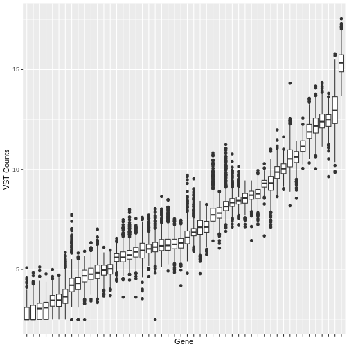
Many machine learning algorithms are sensitive to the scale of the data. Even after having ‘normalised’ RNA-Seq counts data to account for differences in sequence depth and sample composition, and having performed a variance stabilising transformation or rlog transformation to reduce the skewedness and mean-variance relationship, individual genes (variables) will still be on very different scales. The box plot below illustrates this for a small sample of 50 genes from our dataset, with median vst counts ranging from close to zero, to greater than 10.
R
counts.mat.ibd.vst %>%
  as.data.frame() %>%
  tibble::rownames_to_column("geneID")  %>%
  .[sample(nrow(.), size = 50, replace = FALSE),] %>% head(50) %>%
  reshape2::melt(id.vars = 'geneID', value.name='count', variable.name=c('sampleID')) %>%
  ggplot2::ggplot(ggplot2::aes(x = reorder(geneID, count, median), y = count)) +
    ggplot2::geom_boxplot() +
    ggplot2::xlab("Gene") +
    ggplot2::ylab("VST Counts") +
  ggplot2::theme(axis.text.x = ggplot2::element_blank())
In some cases, further scaling of variables will be necessary to put each gene on a similar scale before inputting into a machine learning algorithm. The table below outlines the scenarios where variable scaling will improve the performance of downstream machine learning analysis.
| Scenario | Rationale for Scaling |
|---|---|
| Distance-Based Algorithms | Algorithms that use the Euclidian distance between points to determine the similarity between points require all features to be on the same scale. Without scaling, models will be biased towards features on a larger scale. Examples include clustering techniques: K-Nearest Neighbours, K-means clustering, Principal Component Analysis, and Support Vector Machines |
| Gradient Descent Optimised Algorithms | Algorithms that are optimised using a gradient descent algorithm apply the same learning rate to each variable. Different variable scales will result in very different step sizes across variables, compromising the algorithm’s ability to find a minimum. Linear Regression, Logistic Regression and Neural Networks are all optimised using gradient descent algorithms. |
| Loss Functions with Regularisation Penalties | Machine learning models incorporating a penalty term in the cost function to regularise the model, for example the LASSO, use magnitude of variable coefficients in the penalty term. Without scaling, the penalisation will be biased towards variables on a larger scale. |
On the other hand, there are algorithms that are insensitive to scale where scaling is not necessary. These include tree based models such as Random Forest, XGBoost, Linear Discriminant Analysis and Naive Bayes.
Two widely used rescaling approaches are standardisation (also known as z-scoring), where the distribution of values in every variable is centred around a mean of zero with unit standard deviation, and min-max scaling (confusingly, also known as normalisation) where the values are rescaled to be within the range [0, 1]. In many cases either may be appropriate. The table below gives a few guidelines on when one may be more appropriate than the other.
| Scaling Method | Formula | When more appropriate |
|---|---|---|
| Standardisation | \(\frac{(x - \mu)}{\sigma}\) | - Distribution of the variable data is Gaussian or unknown - Data contains outlier values that would cause the remaining data to be compressed into a very small range if Min-Max scaling is used - The algorithm being used assumes the data has a Gaussian distribution, e.g. linear regression |
| Min-Max Scaling | \(\frac{(x - x_{min})}{x_{max} - x_{min}}\) | - The distribution of the variable data known not to be Gaussian
- The algorithm being used does not make any assumptions about the distribution fo the the data, e.g. neural networks, k-nearest neighbours |
The above is based on a more detailed explanation available at Analytics Vidhya.
Challenge 1:
Test your machine learning knowledge. For each of the following commonly used supervised and unsupervised machine learning algorithms, how would you scale your data, assuming that there were no significant outliers? Would you standardise it, min-max scale it, or leave it unscaled?
- Linear Regression
- Linear Descriminant Analysis
- Logistic Regression
- Support Vector Machines
- Naive Bayes
- K-Nearest-Neighbour
- Decision Trees
- Random Forest
- XGBoost
- Neural Network based models
- Principal Component Analysis
- K-means clustering
| Model | Standardise | Min-Max | Unscaled | Rationale |
|---|---|---|---|---|
| Linear Regression | x | May be optimised by gradient descent; may be regularised with penalty | ||
| Linear Descriminant Analysis | x | Insensitive to scale | ||
| Logistic Regression | x | Optimised by gradient descent; may be regularised with penalty | ||
| Support Vector Machines | x | Distance based; may be optimised by gradient descent; may be regularised with penalty | ||
| Naive Bayes | x | Insensitive to scale, probability (not distance) based | ||
| K-Nearest-Neighbour | x | Distance based; no assumption about data distribution | ||
| Random Forest | x | Insensitive to scale, variables treated individually | ||
| XGBoost | x | Insensitive to scale, variables treated individually | ||
| Neural Network based models | x | Optimised by gradient descent; no assumption about data distribution | ||
| Principal Component Analysis | x | Distance based; may be optimised by gradient descent | ||
| K-means clustering | x | Distance based |
Key Points
- RNA-Seq read count data is heavily skewed with a large percentage of zero values. The distribution is heteroskedastic, meaning the variance depends on the mean.
- Standard transformations such as the variance stabilising transformation and rlog transformation are designed to make the distribution of RNA-Seq data more Gaussian and homoskedastic, which will improve the performance of some machine learning approaches. These transformations are improvements to a simple log2 transformation in particular for low count values.
- Many machine learning algorithms require predictor variables to be on the same scale. Even after vst or rlog transformation, genes in an RNA-Seq dataset will be on very different scales.
- Standardisation (z-score) and min-max scaling are two common techniques to rescale variables.
- Data should be scaled before use with machine learning models that use distance based measures, that include regularisation penalties that utilise absolute values of model coefficients and for models that are optimised via gradient descent. Naive Bayes and tree based models are insensitive to scaling and variables may be left unscaled.