Data Collection: GEO
Last updated on 2024-05-14 | Edit this page
Overview
Questions
- What format are processed RNA-Seq dataset stored on GEO?
- How do I search for a dataset that meets my requirements on GEO?
- How do I use the R package
GEOqueryto download datasets from GEO into R?
Objectives
- Explain the expected data and file formats for processed RNA-Seq datasets on GEO
- Demonstrate ability to correctly identify the subset of files required to create a dataset for a simple supervised machine learning task (e.g., binary classification)
- Demonstrate ability to download and save processed RNA-Seq data files from GEO suitable for a simple supervised machine learning task (e.g., binary classification)
GEO Data Objects
NCBI ‘gene expression omnibus’ , GEO, is one of the largest repositories for functional genomics data. GEO data are stored as individual samples, series of samples and curated datasets. Accession numbers of GEO broadly fall into four categories:
- GSM - GEO Sample. These refer to a single sample.
- GSE - GEO Series. These refer to a list of GEO samples that together form a single experiment.
- GDS - GEO Dataset. These are curated datasets containing summarised information from the underlying GEO samples.
There are many more datasets available as series than there are curated GEO Datasets. For this lesson, we’ll focus on finding a GEO Series as an illustrative dataset.
GEO File Formats
Data for RNA-Seq studies have three components on GEO (similar to microarray studies):
- Metadata
The metadata is equivalent to sample data relationship information provided on ArrayExpress and refers to the descriptive information about the overall study and individual samples. Metadata also contains protocol information and references to the raw and processed data files names for each sample. Metadata is stored in the following standard formats on GEO:
- SOFT (Simple Omnibus Format in Text) is a line-based plain text format
- MINiML is an alternative to SOFT and offers an XML rendering of SOFT
- Series Matrix is a summary text files that include a tab delimited value-matrix table
The raw and processed counts data is typically not included in any of the above files for an RNA-Seq experiement (whereas they may be included with a microarray experiment).
- Processed data files
Processed data (raw counts, noramlised counts) are typically provided in a supplementary file, often a .gz archive of text files. Raw and normalised counts may be provided as separate supplementary files.
- Raw data files
Raw data files provide the original reads and quality scores and are stored in the NIH’s Sequence Read Archive (SRA).
Further information on how RNA-Seq experiments are stored on GEO is given in the submission guidelines on the GEO website.
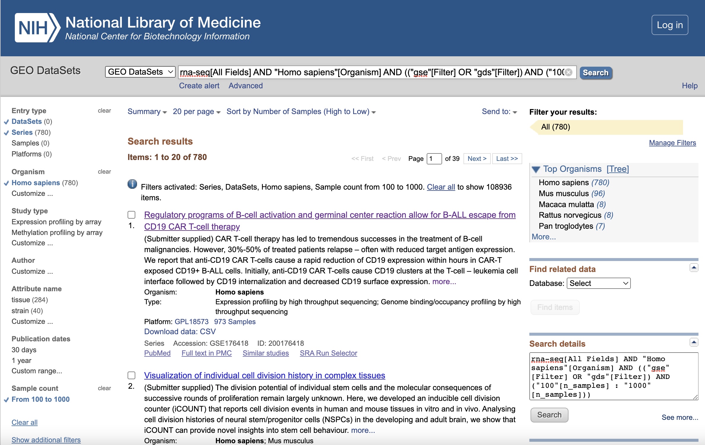
Searching for a Dataset on GEO
Let’s begin on the GEO home page. GEO provides online search and filter tools. We search by adding “rna-seq” as a keyword in the search box, and then apply the following filters to the subsequent results page, and rank the results by the number of samples in descending order:
| Filter | Selection |
|---|---|
| Keywords. | “rna-seq” |
| Entry type | Series or DataSets |
| Organism | homo sapiens |
| Sample count | From 100 to 1,000 |
The full search string is:
rna-seq[All Fields] AND "Homo sapiens"[Organism] AND (("gse"[Filter] OR "gds"[Filter]) AND ("100"[n_samples] : "1000"[n_samples]))
The filtered results page should looks like this:
Illustrative Dataset: Covid-19 Dataset
The data set GSE212041 relates to the case-control study of neutrophils in Covid-19+ patients named “Longitudinal characterization of circulating neutrophils uncovers phenotypes associated with severity in hospitalized COVID-19 patients” and comprises longitudinal human samples from 306 hospitalized COVID-19+ patients, 78 symptomatic controls, and 8 healthy controls, each at multiple time points, with a total of 781 samples. We’ll call it the Covid-19 dataset. Processed data is provided as raw counts and TPM normalised counts in the Supplementary files.
Let’s look at some of the basic information on this dataset:
| Data Field | Values |
|---|---|
| Sample count | 781 |
| Experimental Design | case control design |
| Experimental factors | COVID+, COVID- symptomatic, healthy |
Downloading and Reading into R
Using GEOquery to download a GEO series as an expression set
The function getGEO() from the GEOquery
library provides a convenient way to download GEO SOFT format data into
R. Here we will download the GEO Series GSE212041. This blog provides
additional information on reading
GEO SOFT files into R
If there is more than one SOFT file for a GEO Series,
getGEO() will return a list of datasets. Let’s download
GSE212041.
R
gse212041 <- GEOquery::getGEO("GSE212041")
OUTPUT
Setting options('download.file.method.GEOquery'='auto')OUTPUT
Setting options('GEOquery.inmemory.gpl'=FALSE)OUTPUT
Found 2 file(s)OUTPUT
GSE212041-GPL18573_series_matrix.txt.gzOUTPUT
GSE212041-GPL24676_series_matrix.txt.gzR
sprintf("Number of files downloaded: %i", length(gse212041))
OUTPUT
[1] "Number of files downloaded: 2"R
writeLines(sprintf("file %i: %i samples", 1:2, c(dim(gse212041[[1]])[2], dim(gse212041[[2]])[2])))
OUTPUT
file 1: 16 samples
file 2: 765 samples
Extracting the Metadata
We’ll extract the metadata for the larger dataset (765 samples) and examine the column names to verify that the file contains the expected metadata about the experiment.
R
samp.info.cov19 <- Biobase::pData(gse212041[[2]])

colnames(samp.info.cov19)
OUTPUT
 [1] "title"                   "geo_accession"
 [3] "status"                  "submission_date"
 [5] "last_update_date"        "type"
 [7] "channel_count"           "source_name_ch1"
 [9] "organism_ch1"            "characteristics_ch1"
[11] "characteristics_ch1.1"   "characteristics_ch1.2"
[13] "characteristics_ch1.3"   "characteristics_ch1.4"
[15] "molecule_ch1"            "extract_protocol_ch1"
[17] "extract_protocol_ch1.1"  "taxid_ch1"
[19] "description"             "description.1"
[21] "data_processing"         "data_processing.1"
[23] "data_processing.2"       "data_processing.3"
[25] "data_processing.4"       "platform_id"
[27] "contact_name"            "contact_email"
[29] "contact_phone"           "contact_laboratory"
[31] "contact_institute"       "contact_address"
[33] "contact_city"            "contact_state"
[35] "contact_zip/postal_code" "contact_country"
[37] "data_row_count"          "instrument_model"
[39] "library_selection"       "library_source"
[41] "library_strategy"        "supplementary_file_1"
[43] "acuity.max:ch1"          "cell type:ch1"
[45] "covid-19 status:ch1"     "patient category:ch1"
[47] "time point:ch1"
Getting the Counts Data
If we use the exprs() function to extract the counts
data from the expression slot of the downloaded dataset, we’ll see that
in this data series, the counts matrix is not there. The expression set
only contains a list of the accession numbers of the samples included in
the expression set, but not the actual count data. (The code below
attempts to view a sample of the data).
R
Biobase::exprs(gse212041[[2]])[,1:10]
OUTPUT
     GSM6507615 GSM6507616 GSM6507617 GSM6507618 GSM6507619 GSM6507620
     GSM6507621 GSM6507622 GSM6507623 GSM6507624
We can verify this by looking at the dimensions of the object in the exprs slot.
R
dim(Biobase::exprs(gse212041[[2]]))
OUTPUT
[1] 0 765To get the counts data, we need to download the Supplementary file
(not downloaded by the getGeo() function). The
GEOquery::getGEOSuppFiles() function enables us to view and
download supplementary files attached to a GEO Series (GSE). This
function doesn’t parse the downloaded files, since the file format may
vary between data series.
Set the ‘fetch_files’ argument to FALSE initially to view the available files.
R
GEOquery::getGEOSuppFiles(GEO = "GSE212041",
                          makeDirectory = FALSE,
                          baseDir = "./data",
                          fetch_files = FALSE,
                          filter_regex = NULL
                          )$fname
OUTPUT
[1] "GSE212041_Neutrophil_RNAseq_Count_Matrix.txt.gz" "GSE212041_Neutrophil_RNAseq_TPM_Matrix.txt.gz"
Challenge 2: Download the supplementary files
Now Download the file to your /data subdirectory, by setting
fetch_files to TRUE and apply a filter_regex
of '*Count_Matrix*' to include the raw counts file only.
Read a sample of the file into R and check the dimensions of the file
correspond to the expected number of samples.
R
GEOquery::getGEOSuppFiles(GEO = "GSE212041",
                          makeDirectory = FALSE,
                          baseDir = "./data",
                          fetch_files = TRUE,
                          filter_regex = '*Count_Matrix*'
                          )

raw.counts.cov19 <- read.table(file="data/GSE212041_Neutrophil_RNAseq_Count_Matrix.txt.gz",
                             sep="\t",
                             header=T,
                             fill=T,
                             check.names=F)

sprintf("%i rows, corresponding to transcript IDs", dim(raw.counts.cov19)[1])
sprintf("%i columns, corresponding to samples", dim(raw.counts.cov19)[2])
OUTPUT
[1] "60640 rows, corresponding to transcript IDs"
[1] "783 columns, corresponding to samples"
R
gse157657 <- GEOquery::getGEO("GSE157657")

samp.info.geotb <- Biobase::pData(gse157657[[1]])

GEOquery::getGEOSuppFiles(GEO = "GSE157657",
                          makeDirectory = FALSE,
                          baseDir = "./data",
                          fetch_files = TRUE,
                          filter_regex = NULL
                          )

raw.counts.geotb <- read.table(file="data/GSE157657_norm.data.txt.gz",
                             sep="\t",
                             header=T,
                             fill=T,
                             check.names=F)

sprintf("%i rows, corresponding to transcript IDs", dim(raw.counts.geotb)[1])
sprintf("%i columns, corresponding to samples", dim(raw.counts.geotb)[2])
OUTPUT
[1] "58735 rows, corresponding to transcript IDs"
[1] "761 columns, corresponding to samples"
Hint: you’ll need to refer back to the GEO website to understand how the data has been processed.
The counts data have been normalised and transformed using a variance
stabilising transformation using the DESeq2 R library.
Key Points
- Similar to ArrayExpress, GEO stores samples information and counts
matrices separately. Sample information is typically stored in
SOFTformat, as well as a.txtfile. - Counts data may be stored as raw counts and some further processed form of counts, typically as supplementary files. Always review the documentation to determine what “processed data” refers to for a particular dataset.
-
GEOqueryprovides a convenient way to download files directly from GEO into R.