Linear regression

Overview

Teaching: 60 min
Exercises: 0 min

Questions

• How to construct linear regression in python?

• Continuous or Categorical?

• How to interpret regression result?

Objectives

• Construct linear regression in python.

Fitting Data to a Model

With data points available for certain values, we can build a more general predictive model using linear regression. What we’ll do is fit a linear response to each variable from a data set; in fancy terms,

for $n$ values. A linear regression model makes a few key assumptions:

1. Features are linearly independent of each other.
2. Errors in the regression are normally distributed (rather than biased).
3. Effects are linear functions of inputs.

The model $y$ is an effect or response produced by the features, the predictors, or the values (all meaning more or less the same thing to us). If only one feature $x_1$ is used, this is a simple linear regression; if more than one feature is used, as above, then this is a multiple linear regression.

Linear regression is actually implemented several times in Python libraries. We will use the Python library statsmodels to construct a regression model over a fuel efficiency dataset, which can be loaded from Seaborn with the load_dataset() function. We would like to build a regression model to predict an automobile’s fuel efficiency (in mpg or miles per gallon) from vehicle features.

First, we load and clean the data.

import seaborn as sns
mpg = sns.load_dataset("mpg")

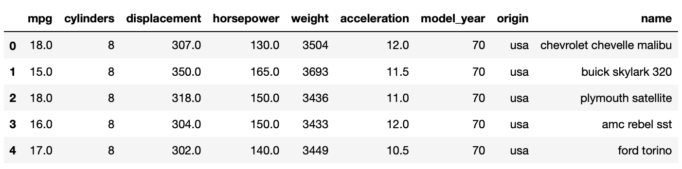
# Display first few rows
mpg.head(5)

Load and examine the data set:

mpg.info()

<class 'pandas.core.frame.DataFrame'>
RangeIndex: 398 entries, 0 to 397
Data columns (total 9 columns):
mpg             398 non-null float64
cylinders       398 non-null int64
displacement    398 non-null float64
horsepower      392 non-null float64
weight          398 non-null int64
acceleration    398 non-null float64
model_year      398 non-null int64
origin          398 non-null object
name            398 non-null object
dtypes: float64(4), int64(3), object(2)
memory usage: 28.1+ KB

The dataset has nine columns, with self-explanatory titles. There are 398 rows in the dataset. One column, horsepower, has 6 missing values. We focus on linear regression in this lesson so we simply drop the rows with missing values to get a clean dataset. (This is by no means the best approach since we will lose valuable data points. One alternative is estimating horsepower by other factors, ie. displacement and acceleration.)

#simply drop missing values
mpg.dropna(inplace=True)
mpg.info()

<class 'pandas.core.frame.DataFrame'>
Int64Index: 392 entries, 0 to 397
Data columns (total 9 columns):
mpg             392 non-null float64
cylinders       392 non-null int64
displacement    392 non-null float64
horsepower      392 non-null float64
weight          392 non-null int64
acceleration    392 non-null float64
model_year      392 non-null int64
origin          392 non-null object
name            392 non-null object
dtypes: float64(4), int64(3), object(2)
memory usage: 30.6+ KB

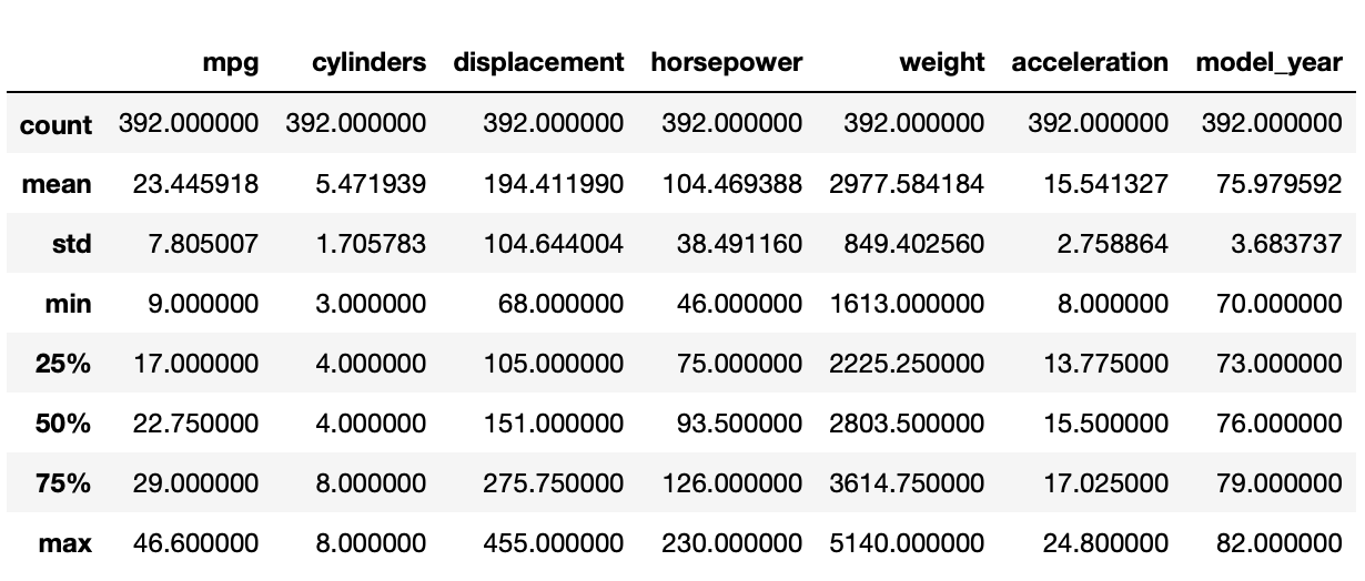
Descriptive Statistics

Our next step is to compute the basic descriptive statistics for the features in this data set. To accomplish this, we can use the .describe() function of the DataFrame.

mpg.describe()

Regression Model

With a clean dataset and a cursory understanding of the basic statistics, we are ready to build a model to predict fuel efficiency. The dependent variable (or response) will be mpg. We need to pick a set of candidate dependent variables from the other eight columns.

There are two types of variables in the dataset, categorical and continuous:

• Categorical Variables: the value is limited and usually based on a particular finite group. E.g., origin.
• Continuous Variables: numeric variables that have an infinite number of gradations between any two values. E.g., horsepower.

In a regression model, dependent variables must be continuous. We don’t have a really great way to handle categorical dependent variables except to create dummy variables for them. Taking origin in this dataset as an example, there are three unique values:

mpg.origin.unique()

array(['usa', 'japan', 'europe'], dtype=object)

To create dummy variables for origin, we can add two new columns to the dataset, say origin_usa and origin_japan.

• If origin is usa, origin_usa=1 and origin_japan=0;
• If origin is japan, origin_usa=0 and origin_japan=1;
• If origin is europe, origin_usa=0 and origin_japan=0.

(Even though there are three distinct values, we only need two dummy columns to cover all the cases.)

statsmodels provides a way to automatically create dummy variables for categorical variables, so we don’t have to do it manually.

For this regression, mpg will be the dependent variable. Let’s choose horsepower, weight and origin for the independent variables. Among these, origin is a categorical variable while the other two are continuous. (Criteria for selecting independent variables can become very complicated.)

To construct the regression model, we define a string-formula using column names (column names can’t have whitespaces). For this dataset and the variables we chose, the formula is defined as:

mpg ~ horsepower + weight + C(origin)

C(origin) indicates that origin is a categorical variable.

We next construct the model using the string formula and the dataset, then fit the model, and display the summary of the regression result.

import statsmodels.formula.api as smf

formula = 'mpg ~ horsepower + weight + C(origin)'
model = smf.ols(formula, data=mpg)
result = model.fit()

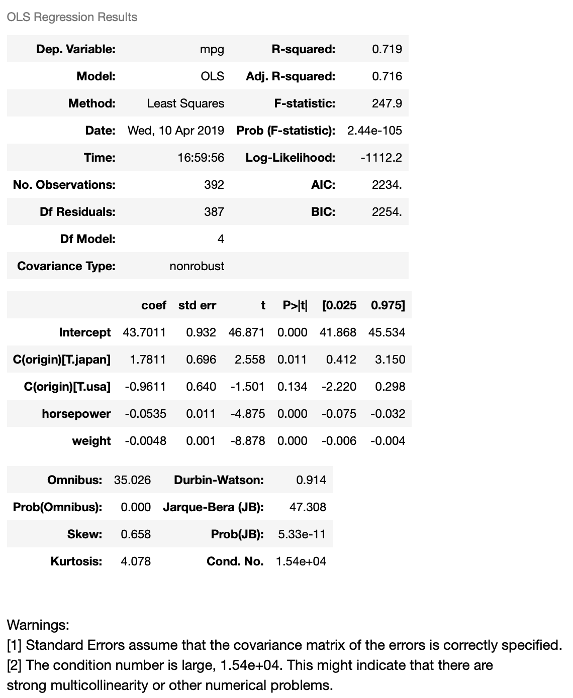
result.summary()

Interpreting Regression Results

The resulting tables shows the dependent variable, the model, and the method. OLS stands for Ordinary Least Squares, meaning that we’re trying to fit a model that minimizes the square of distance of each point from the model regression line.

This model has an $R^2$ value of 0.719, meaning that 71.9% of the variance in our dependent variable (mpg) can be explained by this model.

Based on the coefficient values, we can construct the regression equation:

mpg = 43.7 - 0.0535 horsepower - 0.0048 weight + 1.7811 origin.japan - 0.9611 origin.usa

This reads:

1. If horsepower increases by 1, mpg will decrease by 0.0535.
2. If weight increases by 1 pound, mpg will decrease by 0.0048.
3. If the origin is Japan, mpg will increase by 1.7811 (compared to European cars).
4. If the origin is USA, mpg will decrease by 0.9611 (compared to European cars).

For an European car, origin.japan=0 and origin.usa=0, yielding the equation:

mpg = 43.7 - 0.0535 horsepower - 0.0048 weight

This means that the impact of origin has already been incorporated in the $y$-intercept. This explains why the impact of origin.japan and origin.usa is on top of European cars.

Is model_year categorical or continuous?

Fuel efficiency generally improves over time, so it make sense to consider model_year in the regression model as independent variable. The model_year column contains numeric values, we can add it as a continuous variable. The formula then looks like this:

mpg ~ horsepower + weight + C(origin) + model_year

However, this model assumes that fuel efficiency changes linearly over time, which is not obviously true. It is, in fact, better to add model_year into the regression model as a categorical feature, leadind to the following formula:

mpg ~ horsepower + weight + C(origin) + C(model_year)

We will compare these two models:

formula = 'mpg ~ horsepower + weight + C(origin) + model_year'
model = smf.ols(formula, data=mpg)
result = model.fit()
result.summary()

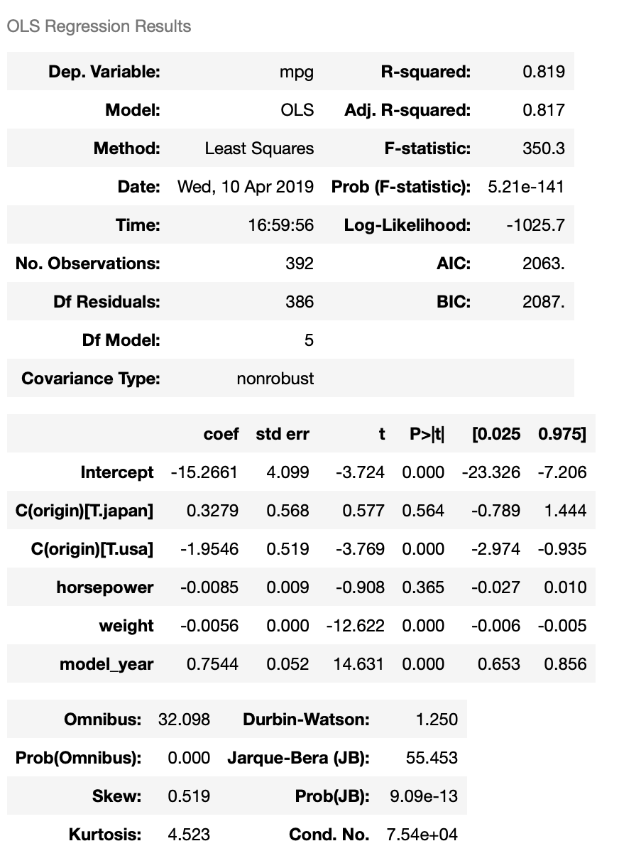
We can see that adding model_year to the model increases $R^2$ from 0.719 to 0.819. The coefficient of model_year is 0.7544, which means mpg increases by 0.7544 each year. The coefficient is also statistically significant. Let’s see what we get when we add model_year to the regression model as a categorical variable.

formula = 'mpg ~ horsepower + weight + C(origin) + C(model_year)'
model = smf.ols(formula, data=mpg)
result = model.fit()
result.summary()

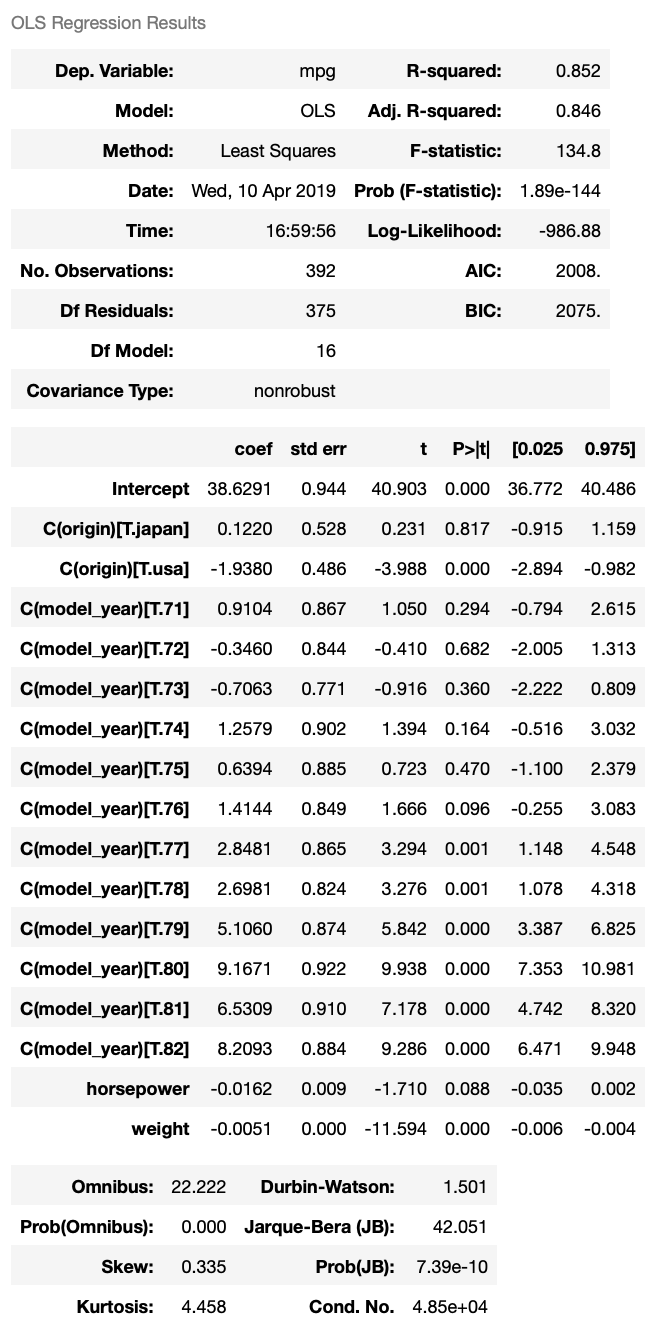
The new model has $R^2 = 0.852$. Looking into the coefficients of dummy variables of model_year, we can see that from 1971 to 1976, there’s not much improvement in vehicle mpg; while from 1977 to 1982, vehicle mpg has significant improvements every year. This model gives better $R^2$, revealing insight into fuel economy changes over time. One drawback of this model is that we can’t predict vehicle gas mileage with it if the vehicle is made after 1982. But overall, we can see that adding model_year as a categorical variable gives us a better regression model.

When we add model_year to the regression model, the coefficient of horsepower is no longer significant. This could indicate that there is multicollinearity between variables, or that horsepower could be explained by other independent variables. This is a very important concept in linear regression that deserves careful investigation to tease out.

Challenge: Determining Impact of Variables

Drop horsepower from the regression model, including only weight, origin and model_year. What is the impact of this change on the model? Why?

Key Points

• Choose independent variables carefully.