Working with Tabular Data
Overview
Teaching: 60 min
Exercises: 0 minQuestions
How do I read a file
What is pandas
How to work with table-like data in Python like Excel
Objectives
Describe what the Python Data Analysis Library (Pandas) is.
Load the Python Data Analysis Library (Pandas).
What’s in our data?
Describe what a DataFrame is in Python.
Access and summarize data stored in a DataFrame.
Merge two dataframes, understand different types of join
Perform basic mathematical operations and summary statistics on data in a Pandas DataFrame.
Create pivot table
Working with Tabular Data
When we read information from a table, we use a casual $x–y$ system to do so: we typically find the record we want (reading down the rows) and then locate the column which contains the value we need to look up. This cleanly separates the two kinds of factors we need to think about: the set of records, and the set of values they contain.

Spreadsheets are valuable because they contain tabular data and allow us to add new fields and relationships. We prefer spreadsheets to be well-organized with only one kind of table in each sheet, and very consistent layout. This makes our tabular data easy for humans to read and (more importantly now) easy for computers to process automatically.
There are some important rules to follow when creating a spreadsheet. Well-formatted data are easier for humans to read and for computer programs to use.
- All variables should be in unique columns across the spreadsheet.
- Each record should be on its own row with data spanning across the sheet.
- Each datum should be in its own cell, which makes processing much easier.
- Work with copies of the raw data, never the raw data themselves.
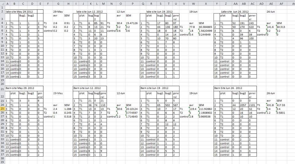
For instance, the following may look like a good table, but because it breaks the rules (how?) it is hard to use with a program.
One of the chief limitations of working with spreadsheets, however, is that they are limited in the number of columns and rows they can manipulate. (At the time of writing, Excel can load 1,048,576 rows and 16,384 columns. This may seem like a lot, but consider common applications like processing transaction records or stock events.) Python is only limited by your computer’s memory in processing data sets.
Another limitation of working with spreadsheets is the automation available. While you can compose macros in Excel, it is often cumbersome to generalize your program away from specific cells, and anyone you share with needs to have the ability to run the same macros. Automatic data manipulation in Python can be shared freely with others and can scale to any new data coming in. It can also help you think very carefully and precisely about the data in terms of the fields (like “Tax Rate” or “Country”) rather than Excel column/row notation (like “A4” and “$B$13”).
Finally, by judiciously using backups of your code, you can trace changes in the development of your analysis procedures. Should you need to work backwards to a previous version, you can easily have that available in a superseded Python file, while spreadsheets don’t store an undo history older than the current session.
The Soft Drink Dataset
We will utilize a dataset representing soft drink sales at a number of convenience stores. Transactions and product data are included.
Please download the dataset for this workshop. You should unzip it to your current working directory. If you are having trouble identifying this, please ask a helper.
We will two files from this dataset in subsequent Python lessons,
item.csvandinvoice.csv.
This dataset contains records with the following fields:
invoice.csv:
| Field | Data Type | Description |
|---|---|---|
| County_id | int |
Unique id for each county |
| County_Name | str |
Name of county |
| City_Name | str |
Name of the city that the county is in |
| Vendor_id | int |
Unique id for each vendor |
| Vendor_Name | str |
Name of the vendor |
| Store_id | int |
Unique id for each store |
| Store_Name | str |
Name of the store |
| Address | str |
Address of the store |
| Zip_Code | int |
Zip code of the store |
| Invoice_id | str |
Unique id for each invoice |
| Date | str |
Date of the invoice |
| Bottle_Sold | int |
Number of bottle sold in the invoice |
| Item_id | int |
Unique id for each item (soda) |
item.csv:
| Field | Data Type | Description |
|---|---|---|
| Item_id | int |
Unique id for each item (soda) |
| Category | str |
Category of soda |
| Item_Description | str |
Name of the item (soda) |
| Pack | int |
Number of bottles that the soda usually sells for |
| Bottle_Volume_ml | float |
Volumn of the soda in ml |
| Bottle_Cost | float |
Cost of one bottle |
| Bottle_Retail_Price | float |
Retile price for one bottle |
These files have the suffix csv. Typically, you are used to seeing xls and xlsx, which are Excel’s preferred formats. csv files are “comma-separated value” files. Run the following command to see what is inside of one of these files—it will show you the first ten lines of data in their raw unprocessed format.
!head -n 10 soda.csv
You can see the tabular structure of the file, and we will take advantage of this to load it into Python using a kind of table called a DataFrame.
The file invoice.csv, incidentally, has about 930,000 records in it, which is under but extremely close to the limit imposed by Excel. If you double-click it to open it in Excel, it will likely take up to 30 seconds to process, and analysis would be similarly mired in difficulties.
Pandas
The Python Data Analysis Library (a.k.a. Pandas) provides tools and data structures for working with tabular data. You will furthermore use it to produce plots, and you can integrate it with other Python libraries for your analysis.
You have seen already that libraries extend Python’s functionality. We will load Pandas and—since the name is a bit cumbersome to type again and again—we will rename it to pd.
import pandas as pd
As before, whenever we use a Pandas-derived function, we need to preface the function with pd..
Reading Tabular Data from csv Files
Our first step is to pull in the data from the file item.csv, which contains product data for the soft drinks.
pd.read_csv("item.csv")
Jupyter recognizes the result of this as a table and displays a well-formatted grid. However, we haven’t stored the result of this function anywhere. Let’s name it soda:
soda = pd.read_csv("item.csv")
Go ahead and load the invoice data now as well.
inv = pd.read_csv("invoice.csv")
Use Python to check the type of one of these:
type(soda)
We call this a DataFrame. You can think of it as a “viewless” spreadsheet—that is, you can access it and manipulate it without needing to see the entire thing laid out.
So What Is a DataFrame?
A
DataFrameis a 2-dimensional data structure that can store data of different types (including characters, integers, floating point values, factors and more) in columns.
Exploring the Dataset
Run
soda
to see the table. It is quite large, and a bit complicated to wrap our heads around. We can see the approximate ranges of values for each field as we scan up and down the records, but displaying the entire table at once is cumbersome. Instead, we can use
soda.head()
to show us only the first few rows of data. Often this is enough to get an idea of the data set.
What kind of data do soda and inv contain? DataFrames have a built-in function info() which can answers this question:
soda.info()
We see how many entries there are for each field and the kind of data stored in each field. The data types don’t quite look familiar based on what we’ve seen before. What should each correspond to in our regular Python types?
Accessing Data Inside a DataFrame
Using our DataFrame
soda, try out the attributes & methods below to see what they return.
soda.columnssoda.shapesoda.tail()
Selecting Data
One of the most common operations in a spreadsheet is to select data. Pandas makes it straightforward to select rows, columns, and internal subsets of data as necessary.
Column. Tradtionally, spreadsheets denote columns by letters. If you want to refer to the field itself, you have to include a column header, and if you are writing a formula, you have to be very careful to use the right column letter.
Using Pandas, the field name (column name, same thing) is a string. Use it as an “index” into the DataFrame to select the entire column:
inv['Store_id']
This returns a Series, which is Pandas’ representation of a single column. It’s a bit simpler than a DataFrame, and mainly notable for requiring an extra step to process sometimes.
To select multiple columns, use a list of columns names as the index.
inv[["Store_id", "Store_Name"]]
Note that this approach returns a DataFrame, not a Series.
Row. Spreadsheets number rows (records). Typically the first field in each record (the first column in each row) is a descriptor of the data set.
Using Pandas, each row is numbered uniquely. You can access a record using its number:
soda.iloc[100]
To make this a bit more intuitive, use the first column as the row label rather than a numeric index. It’s much easier to think about “Cherry Soda” that it is to think about “Row 45.” To do this, we have to reload the data using a special flag called index_col:
soda = pd.read_csv("item.csv",index_col='Item_Description')
inv = pd.read_csv("invoice.csv",index_col='Invoice_id')
Run .info() and .head() again with each of these to see what has changed.
Now when you want to access a row, you can use the record label:
soda.loc["Saitama's Cream Soda"]
(Note that .iloc[] is used with numeric indices while .loc[] is used with row labels.)
Subset. You can use indexing together with field names and record labels to grab particular subsets of data. What would this look like, based on what you know now?
subset = soda[['Bottle_Volume_ml','Bottle_Cost']][soda['Pack']>1]
We can use these selection abilities to produce gradually more complicated formulas for analyzing our data. For instance, to get a list of all of the categories in the soda DataFrame, use
soda['Category']
With this list in hand, we can use pd.unique to extract a list (a Series, really) of how many unique categories there are.
pd.unique(soda['Category'])
Now how would you tell how many unique categories there are?
As in life, there are many ways to accomplish the same end when programming. Instead of using pd.unique, you can use .drop_duplicates:
soda.drop_duplicates("Category")
The difference here is that all other columns are still included.
One more thing: did you notice that one of the values in soda['Category'] isn’t a string? nan means “Not a Number” and is commonly used to mean that a value is missing. The advantage of using nan is that missing data don’t get accidentally included as zeroes, but it can mess up some calculations. To remove them, use
soda['Category'].dropna()
E.g.,
pd.unique(soda['Category'].dropna())
Note that .dropna doesn’t change the underlying data: it returns a modified copy of the data.
Sorting and Filtering Values in DataFrames
Spreadsheets have powerful features for sorting and filtering records based on value. What are the equivalent Python operations?
Sorting. DataFrames can be sorted by one or multiple columns:
# sort by one column:
soda.sort_values(["Bottle_Cost"])

# sort by multiple columns:
soda.sort_values(["Bottle_Cost","Item_Description"])

# sort by multiple columns with different orders in each:
soda.sort_values(["Bottle_Cost","Item_Description"], ascending=[True,False])
How would you sort on bottle cost without nans in the data set?
Challenge: Sorting Both Ways
Produce a
DataFramewhich is sorted in descending order by bottle volume and ascending order by category.Solution
soda.sort_values(["Bottle_Volume_ml","Category"], ascending=[False,True])
Filtering. Filtering describes selecting records based on their values (by range, for instance) or selecting records based on multiple fields.
For instance, select all soft drinks that have a Bottle_Cost less than $3:
soda[soda["Bottle_Cost"]<= 3]["Item_Description"]
soda['Bottle_Cost'] by itself produces a Series of True/False values. These are then used to select only the True values from soda, thus those meeting the filter criterion.
Challenge: Filtering Data
Select all of the sodas with a volume greater than 750 mL.
Solution
soda[soda["Bottle_Volume_ml"] > 750]
Challenge:Challenge: Combining Filters
If we need multiple criteria, we can put parentheses over each criteria and use
&(and) or|(or) to combine the criterias. For example, let’s select sodas that are at least 500ml and cheaper than $3.Solution
soda[(soda["Bottle_Volume_ml"] >= 500) & (soda["Bottle_Cost"]<= 3)]["Item_Description"]
Table Formulas
A very common process in spreadsheet-based analysis is to add new relationships between existing fields. When you add a new formula in a spreadsheet, typically you type it in as a function of other cells: =SUM(A2:D2)/E2. This format obscures the intent of a such a formula and makes it difficult to detect errors.
In Pandas, we will explicity express the relationships between fields using field names:
# calculate the pack price of soft drinks
soda['Pack'] * soda['Bottle_Retail_Price']
This by itself yields a Series. If we want to add this relationship as a new field in the DataFrame, we need to create a new column name and assign the values to it:
soda['Pack_Price'] = soda['Pack'] * soda['Bottle_Retail_Price']
Later on, if you decide that you don’t want this column anymore, you can delete it:
soda = soda.drop(['Pack_Price'], axis = 1)
Calculating Markup
Create a column in the
sodaDataFramethat shows the markup per bottle (price-cost) of each soda.Solution
soda['Markup'] = (soda['Bottle_Retail_Price'] - soda['Bottle_Cost'])
Calculating Profit Margin
Create a column in the
sodaDataFramethat shows the profit margin ((price-cost)/cost) of each soda.Solution
soda['Profit_Margin'] = (soda['Bottle_Retail_Price'] - soda['Bottle_Cost']) / soda['Bottle_Cost']
soda['Profit_Margin'] = soda['Markup'] / soda['Bottle_Cost']
Descriptive Statistics
Let’s carry out some summary statistics to learn more about the data that we’re working with. We often want to calculate summary statistics grouped by subsets or attributes within fields of our data. For example, we might want to calculate the average cost of each soda, or the average volume of each soda which costs more than $4.
We can calculate basic statistics for all records in a single column using the syntax below:
soda['Bottle_Cost'].describe()
yields the output
count    4166.000000
mean        3.648721
std         9.348512
min         1.500000
25%         2.360000
50%         2.860000
75%         3.610000
max       500.000000
Name: Bottle_Cost, dtype: float64
We can also extract one specific metric if we wish:
soda['Bottle_Cost'].min()
soda['Bottle_Cost'].max()
# We can do many other statistic measures such as .std(), .count(), .sum() ... etc
Calculating the Average
Calculate the mean volume of all sodas.
Solution
soda['Bottle_Volume_ml'].mean()
Calculating the Mode
Calculate the mode of volume of all sodas.
Solution
soda['Bottle_Volume_ml'].mode()
Calculating the Average with a Filter
Calculate the mean volume of all sodas which cost more than $4.
Solution
soda[soda['Bottle_Retail_Price']>4]['Bottle_Volume_ml'].mean()
Key Points
Use
read_csvto read tabular data into Python.use sort_values([columns]) to sort the dataframe.
use df_object.column_name or df_object[column_name] to select one column.
use df_object[list_of_column_names] to select multiple columns.
use df_object[condition] to filter data. For example, df_object[df_object[column_name] == value].
use .describe() to get descriptive statistics of one column.
use df1.merge(df2) to merge two DataFrames.
use df_object.groupby(column_list1).agg({column1:agg_function1, column2:agg_function2…}) to apply aggregation on data group.
Create pivot table with pandas.pivot_table