Introduction to Python

Overview

Teaching: 15 min
Exercises: 5 min

Questions

How can I store information?

How can I perform actions?

Objectives

Assign values to variables.

Run built-in functions.

Import libraries.

Using Python

In the following episodes, we will learn the fundamental knowledge to read and run the Python programming language. To run Python commands, we will use a Jupyter Notebook, an interactive platform to run code, write text, and see your results, such as plots. Follow the instructions in the Setup page to open a Notebook.

Variables

In Python, you store information in variables, which have a name and an assigned value.

variable_name = "value" # Here we assign the value to the variable name
variable_name # Here we ask to see the value

'value'

The values can be the result of operations.

new_variable = "a" + "Longer" + "Value"
new_variable

'aLongerValue'

Until now, the data type we have been using is string (str). We saw that summing strings results in a longer combined string. If we work with numerical values the result will be the mathematical one.

a_number = 300
a_number

a_biger_number = 300 + 300
a_biger_number

We can also perform operations with variables that are already set.

a_new_number = a_number + a_biger_number + 100
a_new_number

And if we want to be more efficient, we can assign values to more than one variable in the same line.

color_variable , size_variable = "blue", "big"
color_variable

'blue'

size_variable

'big'

Built-in functions and libraries

Python has basic functions to carry out specific actions. In Python, the arguments of the functions go inside parentheses, and different functions take different kinds and numbers of arguments. The function len() takes one argument and outputs its length. In the case of a string, the length is the number of characters.

len(new_variable)

len(a_number)

---------------------------------------------------------------------------
TypeError                                 Traceback (most recent call last)
/tmp/ipykernel_55271/3566361226.py in <module>
      1 a_number = 300
----> 2 len(a_number)

TypeError: object of type 'int' has no len()

The len() function can give us the number of characters in a string, but it can not do anything with a number (that is of the type int, meaning integer).

Here, you can check the built-in functions of the Python language.

For extra functionalities, there are libraries, which are collections of functions and data structures (see the next episode) specialized in a common set of tasks.

Pandas is an indispensable library specialized in working with tabular data. To make it accessible, you need to import it. There are several ways to import libraries.

Import a library while establishing an alias to access the functions using the alias.

import pandas as pd
pd.read_csv()

Import a library without an alias. You need to access the functions with the complete name of the library.

import pandas
pandas.read_csv()

Import only certain functions from a library. You don’t need to specify a name or alias when calling the function.

from pandas import read_csv
read_csv()

Exercise 1(Begginer): Creating variables and using functions

Create three variables with the common name of your favorite bird as the variable name and the scientific name as the value. Use built-in functions to get the length of the scientific name that has the maximum length.
Solution
swallow, goldcrest, sparrow = "Tachycineta thalassina", "Regulus regulus", "Passer domesticus"
max(len(swallow), len(goldcrest),len(sparrow))
22

Key Points

Variables are Python objects that store information when you assign it to them.

Python has built-in functions that are always accessible.

Libraries give you access to more functions.

Data Structures

Overview

Teaching: 40 min
Exercises: 25 min

Questions

How can I store information in Python?

How can I access the elements of an array or a dictionary?

How can I efficiently manage tabular data in Python?

Objectives

Understand fundamental data structures such as lists, arrays, dictionaries, and Pandas dataframes.

Efficient data manipulation, selection and filtering.

Tabular data management with Pandas.

Read data from a URL.

List

A list is an indexed, ordered, changeable sequence of elements that can be of different types and it allows duplicate values. They are defined using square brackets []:

thislist = ["bacteria", "archea", "fungus", 4]
print(thislist)

['bacteria', 'archea', 'fungus', 4]

To access elements in a list, we can use their index.

first_element = thislist[0]
print(first_element)

bacteria

We can also access elements in the list using negative indices, which count from the end of the list towards the beginning.

print(thislist[-1])

You can add elements to a list using the append() method to add an element to the end of the list.

thislist.append('animal')
print(thislist)

['bacteria', 'archea', 'fungus', 4, 'animal']

You can also extend a list by adding all the elements from another list using the extend() method.

thislist.extend([1,2,3])
print(thislist)

['bacteria', 'archea', 'fungus', 4, 'animal', 1, 2, 3]

You can remove elements from a list using the word del followed by the index of the element you want to remove.

del thislist[3]
print(thislist)

['bacteria', 'archea', 'fungus', 'animal', 1, 2, 3]

You can also use the remove() method to remove a specific element by its value.

thislist.remove('animal')
print(thislist)

['bacteria', 'archea', 'fungus', 1, 2, 3]

You can concatenate two lists using the + operator or the extend() method.

mylist1 = ['bacteria', 'archea', 'fungus']
mylist2 = ['animal', 'algae', 'plant']

newlist = mylist1 + mylist2
print(newlist)

['bacteria', 'archea', 'fungus', 'animal', 'algae', 'plant']

The sort() method sorts the elements of the list in ascending order by default. All elements need to be of the same type. If we try to sort the elements of the list thislist, we will get an error.

thislist.sort()

TypeError: '<' not supported between instances of 'int' and 'str'

newlist.sort()
print(newlist)

['bacteria', 'archea', 'fungus', 'animal', 'algae', 'plant']

To sort them in descending order:

newlist.sort(reverse = True)
print(newlist)

['plant', 'algae', 'animal', 'fungus', 'archea', 'bacteria']

Consider that the sort() method modifies the original list and does not return any value. To sort a list without modifying the original, you can use the sorted() function, which returns a new sorted list.

Select elements of a list with slices
Extra content

Another way to access list data in Python is by using the “slice” method: list[start:end]. This slice includes the elements whose indices are in the range from start to end - 1:

start: It is the index from which we start including elements in the slice.

end: It is the index up to which we include elements in the slice, but not including the element at this index.

For example, if we want to get a slice of newlist from index 1 to index 4, we would use the notation newlist[1:4] and we will get a slice that includes elements from index 1 (inclusive) to index 4 (exclusive).
newlist[1:4]
['algae', 'animal', 'fungus']
Another syntax of “slices” in Python with the notation list[start:end:step] refers to the technique for selecting a subset of elements from a list using three parameters:

start: Indicates the index from which we start including elements in the slice.

end: Indicates the index up to which we include elements in the slice, excluding the element at this index.

step: Indicates the size of the step or increment between the selected elements. That is, how many elements we skip in each step.

If we run newlist[::2], we get a slice that includes elements of the newlist, but selecting every second element. It’s like starting from the beginning of the list, ending at the end, and selecting every second element.
newlist[::2]
['plant', 'animal', 'archea']

Exercise 1(Begginer): Manipulating lists

You are working with genetic data represented by the following list:
genes = ["AGCT", "TCGA", "ATCG", "CGTA"]
How can you remove the sequence “TCGA” and add a new sequence “CATG”? What is the sequence at index 2.
Solution

You can remove “TCGA” from the list using the remove() method:
genes.remove("TCGA")
To add “CATG” to the list, you can use the append() method:
genes.append("CATG")
To find the sequence at index 2, you can access the element at that index using indexing.
sequence_at_index_2 = genes[2]
print(sequence_at_index_2)
CGTA

Dictionary

Dictionaries (dict) are collections of key-value pairs. Each element in the dictionary has a key and an associated value. They are defined using curly braces {} and separating the keys and values with colons :. Dictionaries in Python are mutable, meaning you can add, modify, and delete elements as needed.

thisdict = {
  "brand": "Ford",
  "model": "Mustang",
  "year": 1964
}
print(thisdict)

{'brand': 'Ford', 'model': 'Mustang', 'year': 1964}

You can access the values of the dictionary using their keys.

print(thisdict['brand']) 

Ford

print(thisdict['year'])

If you try to access a key that does not exist in the dictionary, Python will raise a KeyError.

print(thisdict['color'])

KeyError: 'color'

You can add a new key-value pair to the dictionary by simply assigning a value to a new key.

thisdict['color'] = 'red'
print(thisdict)

{'brand': 'Ford', 'model': 'Mustang', 'year': 1964, 'color': 'red'}

You can modify the value associated with an existing key in the dictionary.

thisdict['year'] = 2022
print(thisdict)

{'brand': 'Ford', 'model': 'Mustang', 'year': 2022, 'color': 'red'}

You can delete an item from the dictionary using the del word.

del thisdict['color']
print(thisdict)

{'brand': 'Ford', 'model': 'Mustang', 'year': 2022}

You can also use the pop() method to remove an item and return its value.

thisdict['color'] = 'red'
deleted_value = thisdict.pop('color')
print(deleted_value) 

red

print(thisdict)

{'brand': 'Ford', 'model': 'Mustang', 'year': 2022}

Reserved methods for dictionaries include keys(), values(), and items(). These methods provide convenient ways to access different aspects of a dictionary:

keys(): This method returns a view object that displays a list of all the keys in the dictionary. It allows you to iterate over the keys or convert them into a list if needed.

keys = thisdict.keys()
print(keys)  

dict_keys(['brand', 'model', 'year'])

values(): This method returns a view object that displays a list of all the values in the dictionary. Similar to keys(), it allows iteration over the values or conversion into a list.

values = thisdict.values()
print(values)

dict_values(['Ford', 'Mustang', 2022])

items(): This method returns a view object that displays a list of tuples, where each tuple contains a key-value pair from the dictionary. It’s useful for iterating over both keys and values simultaneously, or for converting the dictionary into a list of key-value pairs.

items = thisdict.items()
print(items) 

dict_items([('brand', 'Ford'), ('model', 'Mustang'), ('year', 2022)])

Modify a dictionary

Extra content

You can modify (update) a dictionary using the update() method. When you call the update() method on a dictionary, you pass another dictionary as an argument. The method then iterates over the key-value pairs in the second dictionary and adds them to the first dictionary. If any keys in the second dictionary already exist in the first dictionary, their corresponding values are updated to the new values.

otherdict = {'model': 'Focus', 'price': 30000}
thisdict.update(otherdict)
print(thisdict)

{'brand': 'Ford', 'model': 'Focus', 'year': 2022, 'price': 30000}

To add new entries to our dictionary, we use the append() method.

thisdict = {
   'brand': ['Ford', 'Toyota'],
   'model': ['Mustang', 'Corolla'],
   'year': [1964, 2020],
   'color': ['red', 'blue'],
   'price': [15000, 20000]
}
# Add a new brand, model, year, color, and price
new_brand = 'Honda'
new_model = 'Civic'
new_year = 2019
new_color = 'green'
new_price = 18000

thisdict['brand'].append(new_brand)
thisdict['model'].append(new_model)
thisdict['year'].append(new_year)
thisdict['color'].append(new_color)
thisdict['price'].append(new_price)

# Print the updated dictionary
print(thisdict)

{'brand': ['Ford', 'Toyota', 'Honda'], 'model': ['Mustang', 'Corolla', 'Civic'], 'year': [1964, 2020, 2019], 'color': ['red', 'blue', 'green'], 'price': [15000, 20000, 18000]}

One way to get the model and year values for each brand is as follows.

# Get the year and model of each car directly from the dictionary
ford_year = thisdict['year'][thisdict['brand'].index('Ford')]
ford_model = thisdict['model'][thisdict['brand'].index('Ford')]

toyota_year = thisdict['year'][thisdict['brand'].index('Toyota')]
toyota_model = thisdict['model'][thisdict['brand'].index('Toyota')]

# Print the year and model of each car
print("Ford's Year:", ford_year)
print("Ford's Model:", ford_model)
print("Toyota's Year:", toyota_year)
print("Toyota's Model:", toyota_model)

Ford's Year: 1964
Ford's Model: Mustang
Toyota's Year: 2020
Toyota's Model: Corolla

Exercise 2(Begginer): Manipulating Dictionaries

Suppose that you have the following dictionary:
genes_dict = {"gene1": { "name": "BRCA1", "start_position": 43044295, "end_position": 43125483},
              "gene2": { "name": "TP53", "start_position": 7571720, "end_position": 7588830},
              "gene3": { "name": "EGFR", "start_position": 55086715, "end_position": 55225454}}
Which command correctly adds a new gene “gene4” with its associated information to an existing genes dictionary in Python?

a) genes_dict.add("gene4", {"name": "GENE4", "start_position": 123456, "end_position": 234567})

b) genes_dict["gene4"] = {"name": "GENE4", "start_position": 123456, "end_position": 234567}

c) genes_dict.append("gene4": {"name": "GENE4", "start_position": 123456, "end_position": 234567})

d) genes_dict.insert(4, {"name": "GENE4", "start_position": 123456, "end_position": 234567})

Solution

The correct answer is option b). It uses the indexing syntax to add a new key-value pair to the genes_dict dictionary, where the key is “gene4” and the value is a dictionary representing the gene’s characteristics.

Array

An method for creating and manipulating multidimensional arrays is by using NumPy. NumPy serves as a foundational library for scientific computing in Python, offering robust support for multidimensional arrays and an extensive array of mathematical functions for efficient memory utilization and rapid numerical operations.

To import it, we use the following.

import numpy as np

To create a one-dimensional array, we use the following.

myarray = np.array([1,2,3,4,5,6])
print(myarray)

[1 2 3 4 5 6]

In NumPy, there are functions to create arrays of zeros or ones. To create an array filled with zeros, you can use np.zeros(shape), where shape is the desired shape of the array:

zeros_array = np.zeros(10)
print(zeros_array)

[0. 0. 0. 0. 0. 0. 0. 0. 0. 0.]

To create an array filled with ones, you can use np.ones(shape).

ones_array = np.ones(10)
print(ones_array)

[1. 1. 1. 1. 1. 1. 1. 1. 1. 1.]

Other ways to create arrays and multidimensional arrays
Extra content

Another way to create arrays is by using sequences with arange(), for example:
np.arange(10)
array([0, 1, 2, 3, 4, 5, 6, 7, 8, 9])
Or using a notation similar to slices: arange(start, stop, step):
np.arange(1,10,1)
array([1, 2, 3, 4, 5, 6, 7, 8, 9])
We can also create them using random values:
np.random.randint(0, 10, 5)
array([9, 6, 0, 2, 7])
Multidimensional arrays can be created in various ways by specifying the dimensions of each dimension. For example, to create a 2-dimensional array filled with zeros, ones, or random values:
array_zeros = np.zeros((3,3))
array_ones = np.ones((3,3))
array_rand = np.random.randint(0,10,(3,3))

print(array_zeros)
print(array_ones)
print(array_rand)
[[0. 0. 0.]
[0. 0. 0.]
[0. 0. 0.]]

[[1. 1. 1.]
[1. 1. 1.]
[1. 1. 1.]]

[[4 5 4]
[1 7 8]
[7 9 9]]
Another way to create a two dimensional array is:
arr_2d = np.array([[1, 2, 3], [4, 5, 6], [7, 8, 9]])
print(arr_2d)
[[1 2 3]
[4 5 6]
[7 8 9]]

The expression len(array) returns the length of the array, which corresponds to the number of elements in the array. For a one-dimensional array, this is the number of elements it contains. For a two-dimensional array, it is the number of rows in the array.

length = len(ones_array)
print(length)

The NumPy library also allows us to load databases using loadtxt. We will use a toy dataset to learn how to import a csv file into a numpy array. The request module is used in Python to make HTTP requests to web servers.

import requests

#  The url to the csv file
url = "https://raw.githubusercontent.com/carpentries-incubator/pangenomics/gh-pages/files/spiral_2d.csv"

# Get the content of the file
response = requests.get(url)
content = response.text

# Load the data into a NumPy array
data = np.loadtxt(content.splitlines(), delimiter=' ')

data

array([[   2.728,    6.513],
       [   3.776,   26.114],
       [   5.595,   38.47 ],
       ...,
       [2003.23 , 1849.23 ],
       [2003.95 , 1928.41 ],
       [2004.09 , 1966.77 ]])

Exercise 3(Begginer): Manipulating arrays

Suppose you have a the following array dna_array containing DNA sequences as strings.
dna_sequences = ["AGCT", "TCGA", "ATCG", "CGTA", "GATTACA"]
dna_array = np.array(dna_sequences)
print(dna_array)
You want to extract the sequences that meet a specific condition. Which NumPy function would you use to extract DNA sequences from dna_array that contain “AT”?

a) np.extract(dna_array == 'AT', dna_array)

b) np.where(dna_array == 'AT')

c) np.extract(np.char.startswith(dna_array, 'AT'), dna_array)

d) dna_array[np.char.count(dna_array, 'AT') > 0]

Solution

The correct is d).

DataFrame

As we see in the first episode, Pandas is an indispensable library specialized in working with tabular data or a DataFrame. We will import the Pandas with its usual alias pd.

import pandas as pd

One form to create a DataFrame is with a dictionary. We will use the dictionary thisdict and then we will convert it to a dataframe.

print(thisdict)

{'brand': ['Ford', 'Toyota', 'Honda'], 'model': ['Mustang', 'Corolla', 'Civic'], 'year': [1964, 2020, 2019], 'color': ['red', 'blue', 'green'], 'price': [15000, 20000, 18000]}

We will add a row name with index.

df = pd.DataFrame(thisdict, index = ['C1', 'C2', 'C3'])
print(df)

     brand    model  year  color  price
C1    Ford  Mustang  1964    red  15000
C2  Toyota  Corolla  2020   blue  20000
C3   Honda    Civic  2019  green  18000

We can explore the dataframe using different methods, such as head(), tail(), info(), describe(), etc. For example:

# Print the first two rows
print(df.head(2))

     brand    model  year color  price
C1    Ford  Mustang  1964   red  15000
C2  Toyota  Corolla  2020  blue  20000

# Print the last two rows
print(df.tail(2))

     brand    model  year  color  price
C2  Toyota  Corolla  2020   blue  20000
C3   Honda    Civic  2019  green  18000

# Display summary statistics
print(df.describe())

              year         price
count     3.000000      3.000000
mean   2001.000000  17666.666667
std      32.046841   2516.611478
min    1964.000000  15000.000000
25%    1991.500000  16500.000000
50%    2019.000000  18000.000000
75%    2019.500000  19000.000000
max    2020.000000  20000.000000

# Display the information of the DataFrame
print(df.info())

<class 'pandas.core.frame.DataFrame'>
Index: 3 entries, C1 to C3
Data columns (total 5 columns):
 #   Column  Non-Null Count  Dtype 
---  ------  --------------  ----- 
 0   brand   3 non-null      object
 1   model   3 non-null      object
 2   year    3 non-null      int64 
 3   color   3 non-null      object
 4   price   3 non-null      int64 
dtypes: int64(2), object(3)
memory usage: 144.0+ bytes
None

Pandas provides different methods for indexing and selecting data from DataFrames. You can use iloc[] for integer-based indexing and loc[] for label-based indexing. For example:

Select columns by name:

print(df['model'])

C1    Mustang
C2    Corolla
C3      Civic
Name: model, dtype: object

Select rows by index using iloc[]

print(df.iloc[1])

brand     Toyota
model    Corolla
year        2020
color       blue
price      20000
Name: C2, dtype: object

Select rows by index name using loc[]

print(df.loc['C1'])

brand       Ford
model    Mustang
year        1964
color        red
price      15000
Name: C1, dtype: object

Select rows and columns with iloc[]

print(df.iloc[0:2, 0:2])

     brand    model
C1    Ford  Mustang
C2  Toyota  Corolla

Select multiple columns.

print(df[['model', 'year']])

      model  year
C1  Mustang  1964
C2  Corolla  2020
C3    Civic  2019

We can filter the data by some conditions. For example:

print(df[df['year']> 2000])

     brand    model  year  color  price
C2  Toyota  Corolla  2020   blue  20000
C3   Honda    Civic  2019  green  18000

We can modify DataFrames by adding or removing rows and columns, updating values, and performing various data transformations. For example:

# Add a column
df['mileage'] = [150000, 5000, 30000]
print(df)

     brand    model  year  color  price  mileage
C1    Ford  Mustang  1964    red  15000   150000
C2  Toyota  Corolla  2020   blue  20000     5000
C3   Honda    Civic  2019  green  18000    30000

# Remove a column from the DataFrame
df.drop(columns=['color'], inplace=True)

print(df)

     brand    model  year  price  mileage
C1    Ford  Mustang  1964  15000   150000
C2  Toyota  Corolla  2020  20000     5000
C3   Honda    Civic  2019  18000    30000

# Update values in a DataFrame
df.loc[df['model'] == 'Corolla', 'mileage'] = 25000

print(df)

     brand    model  year  price  mileage
C1    Ford  Mustang  1964  15000   150000
C2  Toyota  Corolla  2020  20000    25000
C3   Honda    Civic  2019  18000    30000

Just like with numpy, we can read CSV files that are stored on our computer or on the internet.

# Read the url database
url = "https://raw.githubusercontent.com/carpentries-incubator/pangenomics/gh-pages/files/familias_minis.csv"
df_genes = pd.read_csv(url, index_col=0)
df_genes.head(5)

                                  g_A909               g_2603V               g_515               g_NEM316
A909|MGIDGNCP_01408  A909|MGIDGNCP_01408  2603V|GBPINHCM_01420   515|LHMFJANI_01310  NEM316|AOGPFIKH_01528
A909|MGIDGNCP_00096  A909|MGIDGNCP_00096  2603V|GBPINHCM_00097   515|LHMFJANI_00097  NEM316|AOGPFIKH_00098
A909|MGIDGNCP_01343  A909|MGIDGNCP_01343                   NaN                  NaN  NEM316|AOGPFIKH_01415
A909|MGIDGNCP_01221  A909|MGIDGNCP_01221                   NaN   515|LHMFJANI_01130                    NaN
A909|MGIDGNCP_01268  A909|MGIDGNCP_01268  2603V|GBPINHCM_01231   515|LHMFJANI_01178  NEM316|AOGPFIKH_01341  

Exercise 4(Advanced): Manipulating dataframes

Use the dataframe df_genes and add a column that counts how many genes are in each row, for example, the first row has 4 genes but the third row has only two.
Solution

With the following command you can add a column. The method count counts how many elements there are per row, with axis = 1 we can fix the column.
df_genes['Number of genes'] = df_genes.count(axis=1)

Another data structures: Sets and Tuples
Extra content

Tuple

Tuples are indexed and ordered sequences, they are immutable, meaning they cannot be modified after creation. The elements of a tuple can be numbers, strings, or combinations of both types. A tuple is defined using parentheses ():
thistuple = ("bacteria", "archea", "fungus", 3)
print(thistuple)
('bacteria', 'archea', 'fungus', 3)
To access the elements of a tuple, we can use its index. In Python, indexing typically starts at 0. This means that the first element in a sequence (such as a list, tuple, or string) has an index of 0, the second element has an index of 1, and so on.
first_element = thistuple[0]
print(first_element)
bacteria
We can also access tuple elements using negative indices, which count from the end of the tuple towards the beginning.
print(thistuple[-1])
3
Set

Sets are unindexed, unordered collections of unique element, duplicates are not allowed. The sets can contain different data types. They are defined using curly braces {}:
myset = {"bacteria", "archea", "fungus", 4}
print(myset)
{'archea', 3, 'fungus', 'bacteria'}
Sets in Python are mutable, meaning you can add and remove elements, but you cannot directly modify existing elements. To add elements to a set, you can use the add() method.
myset.add('animal')
print(myset)
{3, 'fungus', 'bacteria', 'animal', 'archea'}
To remove an element from a set, you can use the remove().
myset.remove(3)
print(myset)
{'fungus', 'bacteria', 'animal', 'archea'}
Sets are useful when you need to store a collection of unique elements and perform efficient set operations such as removing duplicates and comparing collections.

Key Points

Gain familiarity with fundamental data structures such as tuples, sets, lists, dictionaries, and arrays.

Develop skills in manipulating data by accessing, modifying, and filtering elements within data structures.

Learn to work with tabular data using Pandas DataFrames, including loading and exploring data.

Functions

Overview

Teaching: 20 min
Exercises: 20 min

Questions

How can evaluate a condition?

How can I repeat an action?

How can create my custom functions?

Objectives

Use the if conditional to decide an action

Use the for loop to iterate actions

Create your functions

If statements

The if statement is a conditional statement in Python that allows us to execute a block of code only if a certain condition is true. It follows this syntax:

if condition:
    # code block to execute if condition is True

Let’s look at whether the two characters representing nucleotides are equal.

char1='A'
char2='A'

if char1 == char2:
    print( char1,"equal", char2)

The else conditional executes a block when the condition in the if is not true.

char1='A'
char1='G'

if char1 == char2:
    print( char1,"equal", char2)
else:
    print( char1,"is not equal", char2)

 A is not equal G

You can add as many instructions inside the if as you want by indenting the sentences. Just remember always to keep the same amount of characters in the indentation.

Exercise 1(Begginer): Evaluate if two strings have equal length

Fill in the blanks to evaluate if the following strings have equal lengths.
str1="ACGT"
str2="GATAKA"

__ ___(____) != ___(____):
      print("Strings does not have equal length")
Solution
if len(str1) != len(str2):
    print(str1,str2)
    print("Strings does not have equal length")

For loops

The for loop is used in Python to iterate over a sequence (such as a list, tuple, string, etc.) and execute a block of code for each element in the sequence. It follows this syntax:

for item in sequence:
    # code block to execute for each item

str1="ACGTAC"
distance=0
for char in str1:
    print("The character is",char)

str1="ACGTAC"
str2="GATAKA"
distance=0
for char1, char2 in zip(str1, str2):
    # If the characters are different, increment the distance
    if char1 != char2:
        distance += 1

Functions

Apart from the built-in functions and the library functions, you can make your functions, first, you define them, and then you use them. To define a function you need to give it a name, say what information you need to feed to it, and what output you want.

Here we will wrap the conditional to decide if two characters are equal in the function equal_chars. First, we defined the function and then we called it.

def equal_chars(character1, character2):
    value=""
    if character1 == character2:
        value="equal"
    else:
        value="Not equal"

    return value

char1='A'
char1='G'

equal_chars(char1,char2)

After we create our first function, Let’s create a hamming distance function for two strings. The function hamming_distance() takes two parameters: str1 and str2, the two strings for which the Hamming distance is calculated.

First, we check if the lengths of the two strings are equal. If they are not equal, we raise a ValueError because the Hamming distance is only defined for strings of equal length. We initialize a variable distance to store the Hamming distance. We then iterate over the characters of the two strings using the zip() function, which pairs the corresponding elements of the two strings together. For each pair of characters, if they are different, we increment the distance variable. Finally, we return the calculated Hamming distance. You can use this function to calculate the Hamming distance between any two strings in Python.

def hamming_distance(str1, str2):
    # Check if the strings have equal length
    if len(str1) != len(str2):
        raise ValueError("Strings must have equal length")

    # Initialize the Hamming distance to 0
    distance = 0

    # Iterate over the characters of the strings
    for char1, char2 in zip(str1, str2):
        # If the characters are different, increment the distance
        if char1 != char2:
            distance += 1

    # Return the calculated Hamming distance
    return distance

Now lets add a multiline comment documenting the parameters needed for the fucntion.

def hamming_distance(str1, str2):
    """
    Calculate the Hamming distance between two strings.

    Parameters:
    str1 (str): First string
    str2 (str): Second string

    Returns:
    int: Hamming distance between the two strings
    """
    # Check if the strings have equal length
    if len(str1) != len(str2):
        raise ValueError("Strings must have equal length")

    # Initialize the Hamming distance to 0
    distance = 0

    # Iterate over the characters of the strings
    for char1, char2 in zip(str1, str2):
        # If the characters are different, increment the distance
        if char1 != char2:
            distance += 1

    # Return the calculated Hamming distance
    return distance

Exercise 2(Intermediate): Sort the function to count the nucleotides in a string

  return nucleotide_counts  
   nucleotide_counts = {'A': 0, 'C': 0, 'G': 0, 'T': 0}

     if nucleotide in nucleotide_counts:
   for nucleotide in sequence:
           nucleotide_counts[nucleotide] += 1

 def calculate_nucleotide_frequency(sequence):

Solution

def calculate_nucleotide_frequency(sequence):
    nucleotide_counts = {'A': 0, 'C': 0, 'G': 0, 'T': 0}

    for nucleotide in sequence:
       if nucleotide in nucleotide_counts:
            nucleotide_counts[nucleotide] += 1

   return nucleotide_counts

Combining the data types you just learned, it is possible to automatize the function even more. Suppose that “population” is a numpy ndarray with genomes as rows. Genomes are represented with only two characters: 1 and 0.

Exercise 3(Intermediate): Sort the comments to document a Hamming distance function for matrixes

# The Hamming distance is multiplied by the number of genes to convert it into an absolute distance
 # Number of genomes 
 # Calculate the Hamming distance between each pair of genomes
 # Saving the distance in the matrix
 # Create an empty matrix for Hamming distances
 
 def calculate_hamming_matrix(population):
    # COMMENT 1
    num_genomes = population.shape[0]
    # COMMENT 2
    hamming_matrix = np.zeros((num_genomes, num_genomes), dtype=int)
    # COMMENT 3
    for i in range(num_genomes):
        for j in range(i+1, num_genomes):  # j=i+1 to avoid calculating the same distance twice
            #COMMENT 4
            distance = hamming(population[i], population[j]) * len(population[i])
            hamming_matrix[i, j] = distance # COMMENT 5
            hamming_matrix[j, i] = distance  # The matrix is symmetric
     
    return hamming_matrix

Solution

def calculate_hamming_matrix(population):
   # Number of genomes
   num_genomes = population.shape[0]
   # Create an empty matrix for Hamming distances
   hamming_matrix = np.zeros((num_genomes, num_genomes), dtype=int)
   # Calculate the Hamming distance between each pair of genomes
   for i in range(num_genomes):
       for j in range(i+1, num_genomes):  # j=i+1 to avoid calculating the same distance twice
           # The Hamming distance is multiplied by the number of genes to convert it into an absolute distance
           distance = hamming(population[i], population[j]) * len(population[i])
           hamming_matrix[i, j] = distance
           hamming_matrix[j, i] = distance  # The matrix is symmetric
   return hamming_matrix

Key Points

The conditional if evaluates a statement and performs an action

The for loop repeats an action a predetermined number of times

Custom functions can be defined with def

Plotting

Overview

Teaching: 25 min
Exercises: 15 min

Questions

How can I plot histograms

How can I plot a graph with vertex and edges

Objectives

Create a graph with matplotlib

Create a graph with NetworkX

Python has several libraries that plot and visualize data. NetworkX is a library for working with graph data structures and algorithms, Plotly is a library for creating interactive and publication-quality plots, and Matplotlib is a comprehensive plotting library for creating static and interactive visualizations in Python. Each of these libraries serves different purposes and can be used for various data visualization tasks depending on the requirements and preferences of the user.

Plot with matplotlib

First, we import the matplotlib.pyplot module, which provides a MATLAB-like plotting interface.

import matplotlib.pyplot as plt

Now, we defined some sample data for which we wanted to create a histogram.

data = [1, 2, 2, 3, 3, 3, 4, 4, 4, 4, 5, 5, 5, 5, 5]
print(data)

[1, 2, 2, 3, 3, 3, 4, 4, 4, 4, 5, 5, 5, 5, 5]

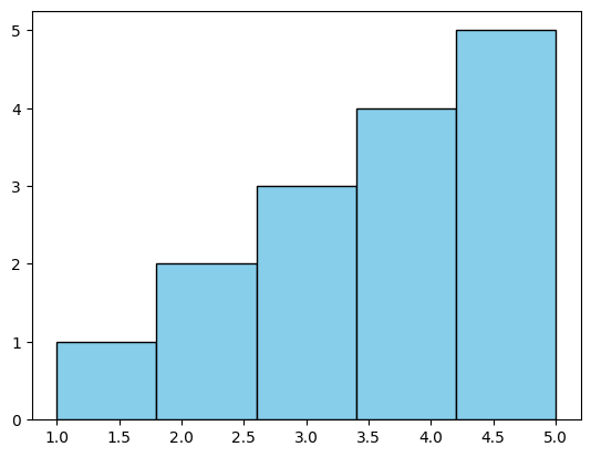
We use the plt.hist() function to create the histogram. We pass the data as the first argument, specify the number of bins using the bins parameter, and optionally specify the color of the bars and their edges using the color and edgecolor parameters, respectively.

plt.hist(data, bins=5, color='skyblue', edgecolor='black')

(array([1., 2., 3., 4., 5.]),
 array([1. , 1.8, 2.6, 3.4, 4.2, 5. ]),
 <BarContainer object of 5 artists>)

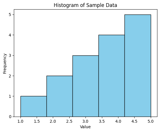
We add labels to the x-axis and y-axis using plt.xlabel() and plt.ylabel(), and we add a title to the plot using plt.title().

plt.xlabel('Value')
plt.ylabel('Frequency')
plt.title('Histogram of Sample Data')
plt.hist(data, bins=5, color='skyblue', edgecolor='black')

(array([1., 2., 3., 4., 5.]),
 array([1. , 1.8, 2.6, 3.4, 4.2, 5. ]),
 <BarContainer object of 5 artists>)

Notice that if you are not in colab or Jupyter Notebook, but in stand-alone Python you will need plt.show() to display the plot.

plt.show()

In this example, we produced a simple histogram of the sample data with five bins, with each bin representing the frequency of values falling within its range. The bars were colored sky blue with black edges for better visibility.

Exercise 1(Begginer): The nucleotide frequency of a DNA sequence

In the DNA sequence stored in the string dna_sequence, we want to graph the frequency of each nucleotide. Sort and fill in the blanks in the following code to get the frequency plot. Notice that we are using the function nucleotide_counts, which we constructed in the previous episode
Figure 5. Histogram of the nucleotide frequency on a DNA sequence.
plt.bar(__________, __________, color='skyblue')
frequencies = list(nucleotide_counts.values())
nucleotide_counts = calculate_nucleotide_frequency(_______)
dna_sequence = "ATGCTGACCTGAAGCTAAGCTAGGCT"  
nucleotides = ____(nucleotide_counts.keys())
Solution
   nucleotide_counts = calculate_nucleotide_frequency(dna_sequence)
   nucleotides = list(nucleotide_counts.keys())
   frequencies = list(nucleotide_counts.values())

   plt.xlabel('Nucleotide')
   plt.ylabel('Frequency')
   plt.title('Nucleotide Frequency Histogram')
   plt.bar(nucleotides, frequencies, color='skyblue')

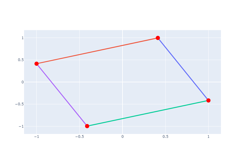
Creating graphs with NetworkX and Plotly

Let’s create a simple graph with NetworkX and visualize it using Plotly. In this example, we’ll create a graph with four nodes and four edges. Nodes are represented as red markers, and edges are represented as black lines.

import networkx as nx
import plotly.graph_objects as go

We create a simple undirected graph G.

# Create a simple graph
G = nx.Graph()
G.add_edges_from([(1, 2), (2, 3), (3, 4), (4, 1)])

We define positions for nodes using a spring layout algorithm (spring_layout). This assigns positions to nodes in such a way that minimizes the forces between them, resulting in a visually appealing layout.

When you call nx.spring_layout(G) without specifying any arguments, the layout is generated randomly each time the function is called. However, if you want to ensure that you get the same layout each time you generate it, you can set a seed for the random number generator.

# Define positions for nodes
# Set a seed for the random number generator
seed_value = 42  # Choose any integer value as the seed
pos = nx.spring_layout(G, seed=seed_value)
pos

{1: array([0.4112362 , 0.99648922]),
array([ 1.        , -0.41570474]),
array([-0.41137359, -0.99514183]),
array([-0.99986261,  0.41435735])}

Try removing or changing the seed_value; what do you observe?

We create traces for edges and nodes. Each edge is represented by a line connecting the positions of its two endpoints, and each node is represented by a marker at its position.

# Create edge traces
edge_traces = []
for edge in G.edges():
    x0, y0 = pos[edge[0]]
    x1, y1 = pos[edge[1]]
    edge_trace = go.Scatter(x=[x0, x1], y=[y0, y1], mode='lines', line=dict(width=3))
    edge_traces.append(edge_trace)

edge_traces

[Scatter({
     'line': {'width': 3},
      'mode': 'lines',
      'x': [0.4112362006825586, 1.0],
      'y': [0.9964892191512681, -0.41570474278971886]
 }),
 Scatter({
     'line': {'width': 3},
     'mode': 'lines',
     'x': [0.4112362006825586, -0.9998626088117056],
     'y': [0.9964892191512681, 0.41435735265600393]
 }),
 Scatter({
     'line': {'width': 3},
     'mode': 'lines',
     'x': [1.0, -0.4113735918708533],
     'y': [-0.41570474278971886, -0.9951418290175523]
 }),
 Scatter({
     'line': {'width': 3},
     'mode': 'lines',
     'x': [-0.4113735918708533, -0.9998626088117056],
     'y': [-0.9951418290175523, 0.41435735265600393]
 })]
Productos pagados de Colab - Cancela los contratos aquí

We create a Plotly figure with the specified data and layout. We disable the legend for simplicity.

node_x = []
node_y = []
for node in G.nodes():
    x, y = pos[node]
    node_x.append(x)
    node_y.append(y)

node_trace = go.Scatter(x=node_x, y=node_y, mode='markers', marker=dict(size=14, color='rgb(255,0,0)'))

print("node_x",node_x)
print("node_y",node_y)

node_x [0.4112362006825586, 1.0, -0.4113735918708533, -0.9998626088117056]
node_y [0.9964892191512681, -0.41570474278971886, -0.9951418290175523, 0.41435735265600393]

Let’s create the Plotly figure and show it using Plotly’s show() method.

fig = go.Figure(data=edge_traces + [node_trace], layout=go.Layout(showlegend=False))
fig.show()

In the Topological Data Analysis for Pangenomics lesson, we need to graph and color triangles beside edges and nodes. Let’s do an example with NetworkX. First, we define two triangles, one with vertexes (1,2,3) and another with vertexes in nodes (4,3,2) of the above object.

triangles = [(1, 2, 3), (4, 3, 2)] # Define some triangles (example)

Now, we will use node_trace to define some characteristics of the nodes in the graph. Each node is represented by a marker (dot) with a corresponding text label displayed above it. The parameters used in its creation control various aspects of the appearance and behavior of the markers and text labels.

x=[] and y=[]: These parameters specify the x and y coordinates of the nodes in the scatter plot. Since we’re defining a trace for nodes, these lists are initially empty. The actual coordinates of the nodes will be added later based on the graph’s layout.
mode=’markers+text’: This parameter specifies the scatter plot’s mode. markers+text indicates that markers (dots representing nodes) and text labels will be displayed for each node.
hoverinfo=’text’: This parameter specifies what information will be displayed when hovering over a node. In this case, it’s set to ‘text’, meaning the text labels provided for each node will be displayed when hovering over the corresponding marker.
marker=dict(size=14): This parameter specifies the properties of the markers (nodes) in the scatter plot. Here, size=14 indicates the size of the markers.
text=[‘Node 1’, ‘Node 2’, ‘Node 3’]: This parameter specifies the text labels for each node.
textposition=’top center’: This parameter specifies the text’s position relative to the markers.

textfont=dict(size=14): This parameter specifies the font properties of the text labels. Here, size=14 indicates the font size of the text.

# Node trace
node_trace = go.Scatter(x=[], y=[], mode='markers+text', hoverinfo='text', marker=dict(size=14), text=['Node 1', 'Node 2', 'Node 3'], textposition='top center', textfont=dict(size=14))

Now that you know the for cycle, let’s iterate over all edges in the graph, extract the positions of the nodes connected by each edge, and create a scatter plot trace representing the edge with a line connecting the two endpoints. These traces are stored in a list (edge_traces) to be later included in the plot.

# Edge traces
edge_traces = []
for edge in G.edges():
    x0, y0 = pos[edge[0]]
    x1, y1 = pos[edge[1]]
    edge_trace = go.Scatter(x=[x0, x1, None], y=[y0, y1, None], mode='lines', line=dict(width=3, color='rgba(0,0,0,0.5)'))
    edge_traces.append(edge_trace)

Now, we iterate over all triangles in the graph, extract the positions of the vertices of each triangle, and create scatter plot traces representing the triangles as filled polygons with lines connecting the vertices. These traces are stored in a list (triangle_traces) to be later included in the plot.

# Triangle traces
triangle_traces = []
for triangle in triangles:
    x = [pos[vertex][0] for vertex in triangle]
    y = [pos[vertex][1] for vertex in triangle]
    triangle_trace = go.Scatter(x=x + [x[0]], y=y + [y[0]], fill='toself', mode='lines+markers', line=dict(width=2), fillcolor='rgba(255,0,0,0.2)')
    triangle_traces.append(triangle_trace)

Now, we want to configure the plot layout by specifying settings for various components such as the legend, hover behavior, appearance of axes, and font properties of tick labels. These settings are organized into a layout object (layout) using the go.Layout() constructor.

# Configure the layout of the plot
layout = go.Layout(showlegend=False, hovermode='closest', xaxis=dict(showgrid=False, zeroline=False, tickfont=dict(size=16, family='Arial, sans-serif')), yaxis=dict(showgrid=False, zeroline=False, tickfont=dict(size=16, family='Arial, sans-serif')))

To create the figure, we add edges, triangles, and nodes to the data and then use the go.Figure function.

# Create the figure
fig = go.Figure(data=edge_traces + triangle_traces + [node_trace], layout=layout)

Finally, we want to adjust the size of the plot by setting its width and height based on the plot_size and dpi variables.

# Set the figure size
plot_size = 1
dpi = 600
fig.update_layout(width=plot_size * dpi, height=plot_size * dpi)
fig.show() # Show the figure

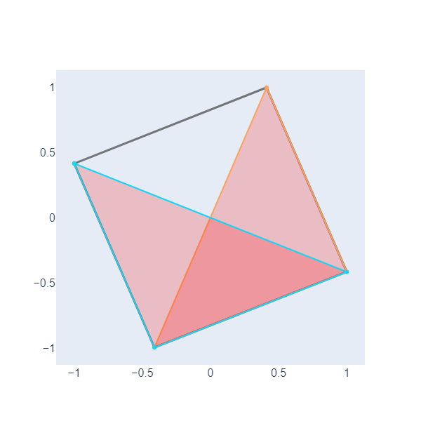
Here, we have plotted two filled triangles, we will need this ability to graph objects called simplicial complexes in the following lesson.

Exercise 2(Intermediate): Documenting a graph plot code

Look at the following function used in the Horizontal Gene transfer episode. 1) Based on what you learned about plotting triangles and edges, sort the comments that document what that part of the code is doing.
COMMENT: Triangle traces
COMMENT: Calculate node positions if not provided
COMMENT: Show the figure
COMMENT: Node trace
COMMENT: Save the figure if a filename is provided
COMMENT: Configure the layout of the plot
COMMENT: Edge traces

3) What do you think the simplex tree contain?
4) what is the save_fiename doing?

def visualize_simplicial_complex(simplex_tree, filtration_value, vertex_names=None, save_filename=None, plot_size=1, dpi=600, pos=None):
   G = nx.Graph()
  triangles = []  # List to store triangles (3-nodes simplices)
  
   for simplex, filt in simplex_tree.get_filtration():
       if filt <= filtration_value:
           if len(simplex) == 2:
               G.add_edge(simplex[0], simplex[1])
           elif len(simplex) == 1:
               G.add_node(simplex[0])
           elif len(simplex) == 3:
               triangles.append(simplex)
   
   # FIRST COMMENT
   if pos is None:
       pos = nx.spring_layout(G)
   
   # SECOND COMMENT
   x_values, y_values = zip(*[pos[node] for node in G.nodes()])
   node_labels = [vertex_names[node] if vertex_names else str(node) for node in G.nodes()]
   node_trace = go.Scatter(x=x_values, y=y_values, mode='markers+text', hoverinfo='text', marker=dict(size=14), text=node_labels, textposition='top center', textfont=dict(size=14))
   
   # THIRD COMMENT
   edge_traces = []
   for edge in G.edges():
       x0, y0 = pos[edge[0]]
       x1, y1 = pos[edge[1]]
       edge_trace = go.Scatter(x=[x0, x1, None], y=[y0, y1, None], mode='lines', line=dict(width=3, color='rgba(0,0,0,0.5)'))
       edge_traces.append(edge_trace)
   
   # FOURTH COMMENT
   triangle_traces = []
   for triangle in triangles:
       x0, y0 = pos[triangle[0]]
       x1, y1 = pos[triangle[1]]
       x2, y2 = pos[triangle[2]]
       triangle_trace = go.Scatter(x=[x0, x1, x2, x0, None], y=[y0, y1, y2, y0, None], fill='toself', mode='lines+markers', line=dict(width=2), fillcolor='rgba(255,0,0,0.2)')
       triangle_traces.append(triangle_trace)
   
   # 5Th COMMENT
   layout = go.Layout(showlegend=False, hovermode='closest', xaxis=dict(showgrid=False, zeroline=False, tickfont=dict(size=16, family='Arial, sans-serif')), yaxis=dict(showgrid=False, zeroline=False, tickfont=dict(size=16, family='Arial, sans-serif')))
   
   fig = go.Figure(data=edge_traces + triangle_traces + [node_trace], layout=layout)
   
   # Set the figure size
   fig.update_layout(width=plot_size * dpi, height=plot_size * dpi)
  
   # 6th COMMENT
   if save_filename:
       pio.write_image(fig, save_filename, width=plot_size * dpi, height=plot_size * dpi, scale=1)
   

  # 7th COMMENT
   fig.show()

  return G

Solution

1) The sorted comments are:
FIRST COMMENT: Calculate node positions if not provided
SECOND COMMENT: Node trace
THIRD COMMENT: Edge traces
FOURTH COMMENT: Triangle traces
5TH COMMENT: Configure the layout of the plot
6TH COMMENT: Save the figure if a filename is provided
7 COMMENT: Show the figure

2) Object simplex_tree contains information about nodes, edges, and triangles
3) Is a parameter to save our graphs in a file

Key Points

matplotlib is a library

NetworkX is a library

Plotting

Overview

Teaching: 25 min
Exercises: 15 min

Questions

How do I create plots in Python?

Objectives

Create basic plots in Python using the Matplotlib library

There are several different Python plotting libraries. Perhaps the most popular one is Matplotlib, initially released back in 2003. Another library, called Seaborn, is based on Matplotlib, and provides “nicer” defaults for colors and plots, making it easier to build beautiful publication-ready plots. A modern alternative is Plotly, that is available not only in Python, but also in R, Julia, JavaScript, MatLab, and F#. This tutorial serves as a brief introduction into Matplotlib.

Introduction to plots: histograms

We’ll use a dataset of reference genomes of Streptomyces. To download it and load it into the Python environment, we can use the Pandas library.

import pandas as pd
data = pd.read_csv("https://raw.githubusercontent.com/carpentries-incubator/pangenomics-python/gh-pages/data/streptomyces.csv")
data

Matplotlib is a large library; however, most plotting functions are available in the matplotlib.pyplot module, which is usually imported as follows.

import matplotlib.pyplot as plt

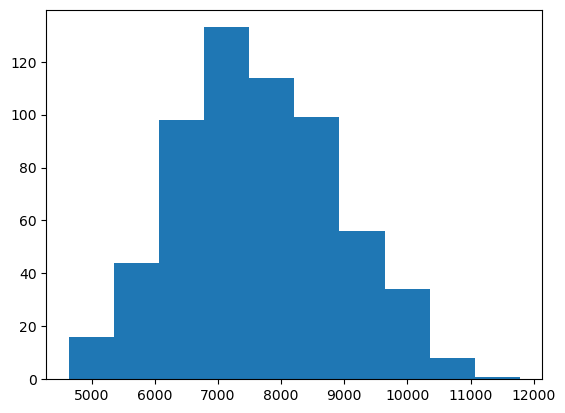
The Matplotlib official website provides a convenient page showing the main plot types available. We’ll begin with a histogram showing the number of genes per reference assembly, which can be accomplished by using the plt.hist function and pass the "genes" column of the dataset, grouping the values automatically. Use the plt.show() function to draw the plot on the screen.

plt.hist(data["genes"])
plt.show()

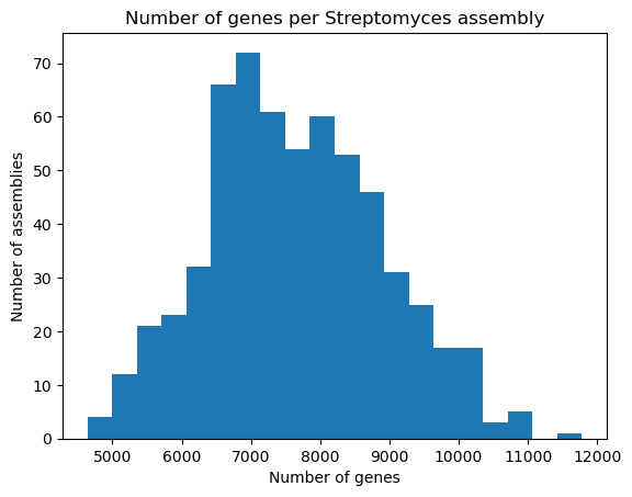
The plt.hist function has many many options that allow you to customize how the chart looks like. For instance, we can use the bins parameter to set the number of bars in the histogram. Furthermore, plots are useless without proper labels, so we’ll use the plt.xlabel, plt.ylabel and plt.title functions to define the label for the x axis, the label for the y axis, and the title for the plot, respectively.

plt.hist(data["genes"], bins=20)
plt.xlabel("Number of genes")
plt.ylabel("Number of assemblies")
plt.title("Number of genes per Streptomyces assembly")
plt.show()

Bars and lines

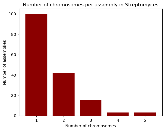
Whereas plt.hist allows you to pass the variables directly, other plot types require you to perform some manipulations on the dataset, because we should explicitly provide both the x and y axes. The plt.bar function, as its name suggests, creates bar plots; we’ll use it to visualize the number of chromosomes per assembly in our dataset. First, we take the "chromosomes" column from the dataset, and use the .value_counts() method to count how many times each chromosome count appears in it. This method returns a Pandas Series, with an index and values which we can access. So, in order to build the bar plot, we first provide the unique chromosome counts for the x axis, and the values for the y axis. We’ll also change the bar colors to dark red and add labels.

chromosomes = data["chromosomes"].value_counts()
chromosomes

chromosomes
0    100
0     42
0     15
0      3
0      3
Name: count, dtype: int64

plt.bar(chromosomes.index, chromosomes.values, color="darkred")
plt.xlabel("Number of chromosomes")
plt.ylabel("Number of assemblies")
plt.title("Number of chromosomes per assembly in Streptomyces")
plt.show()

Going horizontal: creating horizontal bar plots

If you wish to use a horizontal bar plot instead of a vertical one, use the plt.barh function. Don’t forget to change your labels accordingly!

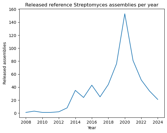
Let’s now learn how to build line plots using plt.plot by visualizing the number of reference assemblies released by year. Similar to the previous example, we’ll use the .value_counts method on the "release_year" columns to count the number of assemblies per year; however, this method sorts the index by the count, so in order to keep the original order (which is already chronological), we pass the sort=False parameter. Next, we provide the index and values for the x and y axes of our plot.

genomes_year = data["release_year"].value_counts(sort=False)
genomes_year

release_year
    1
    3
    1
    1
    2
    8
   35
   24
   43
   25
   44
   76
  153
   81
   51
   34
   21
Name: count, dtype: int64

plt.plot(genomes_year.index, genomes_year.values)
plt.xlabel("Year")
plt.ylabel("Released assemblies")
plt.title("Released reference Streptomyces assemblies per year")
plt.show()

A nice feature about plt.plot is that we can change the way the line looks like, either by modifying the edges and/or the vertices. You can find the format guide in the “Format Strings” section of the function’s documentation. Some example strings you can use are depicted in the next code block.

"--"    # Dashed line
":"     # Dotted line
"o"     # Large dots only
"v"     # Down-facing triangles only
"s"     # Squares only
"--o"   # Dashed line with large dots
":s"    # Dotted line with squares

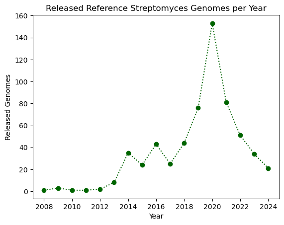
Let’s modify our plot by making it dotted with large dots, with a dark green color.

plt.plot(genomes_year.index, genomes_year.values, ':o', color="darkgreen")
plt.xlabel("Year")
plt.ylabel("Released Genomes")
plt.title("Released Reference Streptomyces Genomes per Year")
plt.show()

Exercise (Beginner): Plotting with Matplotlib

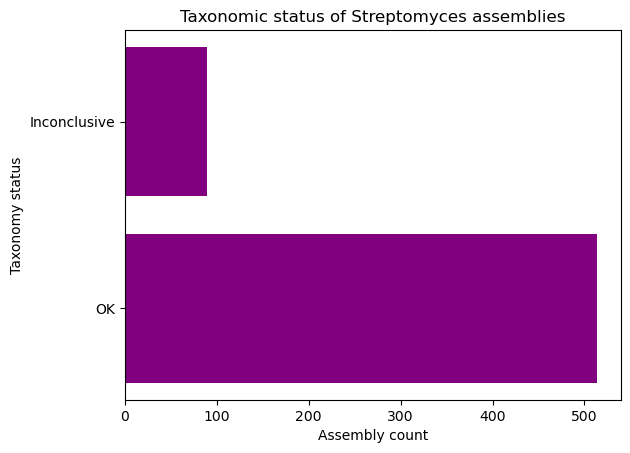
Complete the following code block to create a horizontal bar plot with the number of assemblies with conclusive and inconclusive taxonomy from the dataset. Use purple to color the bars.
taxonomy = data["taxonomy_status"].________()
plt.________(taxonomy.________, taxonomy.__________, ________="purple")
plt.________("Taxonomy status")
plt.________("Assembly count")
plt.title("Taxonomic status of Streptomyces assemblies")
plt.show()
Solution
taxonomy = data["taxonomy_status"].value_counts()
plt.barh(taxonomy.index, taxonomy.values, color="purple")
plt.ylabel("Taxonomy status")
plt.xlabel("Assembly count")
plt.title("Taxonomic status of Streptomyces assemblies")
plt.show()

Multiple plots in a single figure
Extra content

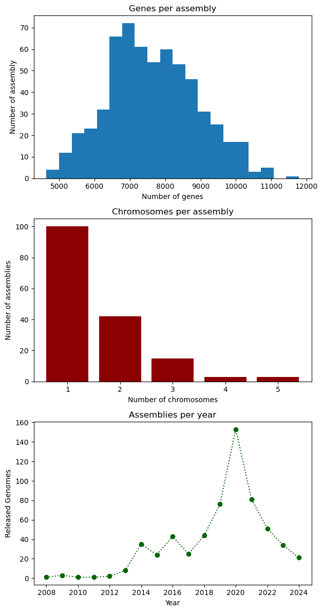
The plt.subplots(x, y) function creates a multi-plot figure with x rows and y columns. It returns a Figure object that allows to modify general aspects of the figure, and an empty array which will store the plots and are accessible via indices. As an example, we’ll create a figure with one column and three rows and place the three plots be made in the lesson. Instead of using .xlabel, .ylabel and .title, we use .set_xlabel, .set_ylabel and .set_title, respectively. At the end, we use the set_figheight method to set the height for the entire figure, and the .tight_layout method on the figure in order to ensure that everything fits in properly.
# Figure initialization
fig, ax = plt.subplots(3)

# First plot: histogram
ax[0].hist(data["genes"], bins=20)
ax[0].set_xlabel("Number of genes")
ax[0].set_ylabel("Number of assembly")
ax[0].set_title("Genes per assembly")

# Second plot: bar
ax[1].bar(chromosomes.index, chromosomes.values, color="darkred")
ax[1].set_xlabel("Number of chromosomes")
ax[1].set_ylabel("Number of assemblies")
ax[1].set_title("Chromosomes per assembly")

# Third plot: line
ax[2].plot(genomes_year.index, genomes_year.values, ':o', color="darkgreen")
ax[2].set_xlabel("Year")
ax[2].set_ylabel("Released Genomes")
ax[2].set_title("Assemblies per year")

# Figure configuration
fig.set_figheight(12)
fig.tight_layout()
plt.show()

Key Points

Matplotlib is a popular plotting library for Python