Introduction to Image Data

Last updated on 2024-05-30 | Edit this page

Overview

Questions

  • How much data do you need for Deep Learning?
  • How do I prepare image data for use in a convolutional neural network (CNN)?
  • How do I work with image data in python?
  • Where can I find image data to train my model?

Objectives

  • Understand the properties of image data.
  • Write code to prepare an image dataset to train a CNN.
  • Know the difference between training, testing, and validation datasets.
  • Identify sources of image data.

Deep Learning Workflow


Let’s start over from the beginning of our workflow.

Step 1. Formulate/ Outline the problem

Firstly we must decide what it is we want our Deep Learning system to do. This lesson is all about image classification and our aim is to put an image into one of ten categories: airplane, automobile, bird, cat, deer, dog, frog, horse, ship, or truck

Step 2. Identify inputs and outputs

Next we identify the inputs and outputs of the neural network. In our case, the data is images and the inputs could be the individual pixels of the images.

We are performing a classification problem and we want to output one category for each image.

Step 3. Prepare data

Deep Learning requires extensive training data which tells the network what output it should produce for a given input. In this workshop, our network will be trained on a series of images and told what they contain. Once the network is trained, it should be able to take another image and correctly classify its contents.

Callout

How much data do you need for Deep Learning?

Unfortunately, this question is not easy to answer. It depends, among other things, on the complexity of the task (which you often do not know beforehand), the quality of the available dataset and the complexity of the network. For complex tasks with large neural networks, adding more data often improves performance. However, this is also not a generic truth: if the data you add is too similar to the data you already have, it will not give much new information to the neural network.

In case you have too little data available to train a complex network from scratch, it is sometimes possible to use a pretrained network that was trained on a similar problem. Another trick is data augmentation, where you expand the dataset with artificial data points that could be real. An example of this is mirroring images when trying to classify cats and dogs. An horizontally mirrored animal retains the label, but exposes a different view.

Depending on your situation, you will prepare your own custom data for training or use pre-existing data.

Custom image data


In some cases, you will create your own set of labelled images.

The steps to prepare your own custom image data include:

Custom data i. Data collection and Labeling:

For image classification the label applies to the entire image; object detection requires bounding boxes around objects of interest, and instance or semantic segmentation requires each pixel to be labelled.

There are a number of open source software used to label your dataset, including:

  • (Visual Geometry Group) VGG Image Annotator (VIA)
  • ImageJ can be extended with plugins for annotation
  • COCO Annotator is designed specifically for creating annotations compatible with Common Objects in Context (COCO) format

Custom data ii. Data preprocessing:

This step involves various tasks to enhance the quality and consistency of the data:

  • Resizing: Resize images to a consistent resolution to ensure uniformity and reduce computational load.

  • Augmentation: Apply random transformations (e.g., rotations, flips, shifts) to create new variations of the same image. This helps improve the model’s robustness and generalisation by exposing it to more diverse data.

  • Normalisation: Scale pixel values to a common range, often between 0 and 1 or -1 and 1. Normalisation helps the model converge faster during training.

  • Label encoding is a technique used to represent categorical data with numerical labels.

  • Data Splitting: Split the data set into separate parts to have one for training, one for evaluating the model’s performance during training, and one reserved for the final evaluation of the model’s performance.

Before jumping into these specific preprocessing tasks, it’s important to understand that images on a computer are stored as numerical representations or simplified versions of the real world. Therefore it’s essential to take some time to understand these numerical abstractions.

Pixels

Images on a computer are stored as rectangular arrays of hundreds, thousands, or millions of discrete “picture elements,” otherwise known as pixels. Each pixel can be thought of as a single square point of coloured light.

For example, consider this image of a Jabiru, with a square area designated by a red box:

Jabiru image that is 552 pixels wide and 573 pixels high. A red square around the neck region indicates the area to zoom in on.

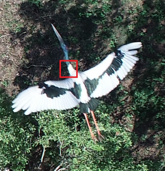
Now, if we zoomed in close enough to the red box, the individual pixels would stand out:

zoomed in area of Jabiru where the individual pixels stand out

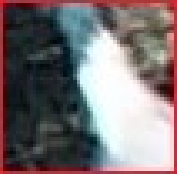
Note each square in the enlarged image area (i.e. each pixel) is all one colour, but each pixel can be a different colour from its neighbours. Viewed from a distance, these pixels seem to blend together to form the image.

Working with Pixels

In python, an image can represented as a 2- or 3-dimensional array. An array is used to store multiple values or elements of the same datatype in a single variable. In the context of images, arrays have dimensions for height, width, and colour channels (if applicable) and each element corresponds to a pixel value in the image. Let us start with the Jabiru image.

PYTHON

# specify the image path
new_img_path = "../data/Jabiru_TGS.JPG"

# read in the image with default arguments
new_img_pil = keras.utils.load_img(path=new_img_path)

# check the image class and size
print('Image class :', new_img_pil.__class__)
print('Image size:', new_img_pil.size)

OUTPUT

Image class : <class 'PIL.JpegImagePlugin.JpegImageFile'>
Image size (552, 573)

Image Dimensions - Resizing

The new image has shape (573, 552), meaning it is much larger in size, 573x552 pixels and is a rectangle instead of a square.

Recall from the introduction that our training data set consists of 50000 images of 32x32 pixels.

To reduce the computational load and ensure all of our images have a uniform size, we need to choose an image resolution (or size in pixels) and ensure all of the images we use are resized to be consistent.

There are a couple of ways to do this in python but one way is to specify the size you want using the target_size argument to the keras.utils.load_img() function.

PYTHON

# read in the image and specify the target size
new_img_pil_small = keras.utils.load_img(path=new_img_path, target_size=(32,32))

# confirm the image class and size
print('Resized image class :', new_img_pil_small.__class__)
print('Resized image size', new_img_pil_small.size) 

OUTPUT

Resized image class : <class 'PIL.Image.Image'>
Resized image size (32, 32)

Of course, if there are a large number of images to preprocess you do not want to copy and paste these steps for each image! Fortunately, Keras has a solution: keras.utils.image_dataset_from_directory()

Two of the most commonly used libraries for image representation and manipulation are NumPy and Pillow (PIL). Additionally, when working with deep learning frameworks like TensorFlow and PyTorch, images are often represented as tensors within these frameworks.

  • NumPy is a powerful library for numerical computing in Python. It provides support for creating and manipulating arrays, which can be used to represent images as multidimensional arrays.
    • import numpy as np
  • The Pillow library provides functions to open, manipulate, and save various image file formats. It represents images using its own Image class.
  • TensorFlow images are often represented as tensors that have dimensions for batch size, height, width, and colour channels. This framework provide tools to load, preprocess, and work with image data seamlessly.
    • from tensorflow import keras
    • image preprocessing documentation
    • Note Keras image functions also use PIL

Image augmentation

There are several ways to augment your data to increase the diversity of the training data and improve model robustness.

  • Geometric Transformations
    • rotation, scaling, zooming, cropping
  • Flipping or Mirroring
    • some classes, like horse, have a different shape when facing left or right and you want your model to recognize both
  • Colour properties
    • brightness, contrast, or hue
    • these changes simulate variations in lighting conditions

We will not perform image augmentation in this lesson, but it is important that you are aware of this type of data preparation because it can make a big difference in your model’s ability to predict outside of your training data.

Information about these operations are included in the Keras document for Image augmentation layers.

Normalisation

Image RGB values are between 0 and 255. As input for neural networks, it is better to have small input values. The process of converting the RGB values to be between 0 and 1 is called normalisation.

Before we can normalise our image values we must convert the image to an numpy array.

We introduced how to do this in Episode 01 Introduction to Deep Learning but what you may not have noticed is that the keras.datasets.cifar10.load_data() function did the conversion for us whereas now we will do it ourselves.

PYTHON

# first convert the image into an array for normalisation
new_img_arr = keras.utils.img_to_array(new_img_pil_small)

# confirm the image class and shape
print('Converted image class  :', new_img_arr.__class__)
print('Converted image shape', new_img_arr.shape)

OUTPUT

Converted image class  : <class 'numpy.ndarray'>
Converted image shape (32, 32, 3)

Now that the image is an array, we can normalise the values. Let us also investigate the image values before and after we normalise them.

PYTHON

# inspect pixel values before and after normalisation

# extract the min, max, and mean pixel values BEFORE
print('BEFORE normalisation')
print('Min pixel value ', new_img_arr.min()) 
print('Max pixel value ', new_img_arr.max())
print('Mean pixel value ', new_img_arr.mean().round())

# normalise the RGB values to be between 0 and 1
new_img_arr_norm = new_img_arr / 255.0

# extract the min, max, and mean pixel values AFTER
print('AFTER normalisation') 
print('Min pixel value ', new_img_arr_norm.min()) 
print('Max pixel value ', new_img_arr_norm.max())
print('Mean pixel value ', new_img_arr_norm.mean().round())

OUTPUT

BEFORE normalisation
Min pixel value  0.0
Max pixel value  255.0
Mean pixel value  87.0
AFTER normalisation
Min pixel value  0.0
Max pixel value  1.0
Mean pixel value  0.0

ChatGPT

Normalizing the RGB values to be between 0 and 1 is a common pre-processing step in machine learning tasks, especially when dealing with image data. This normalisation has several benefits:

  1. Numerical Stability: By scaling the RGB values to a range between 0 and 1, you avoid potential numerical instability issues that can arise when working with large values. Neural networks and many other machine learning algorithms are sensitive to the scale of input features, and normalizing helps to keep the values within a manageable range.

  2. Faster Convergence: Normalizing the RGB values often helps in faster convergence during the training process. Neural networks and other optimisation algorithms rely on gradient descent techniques, and having inputs in a consistent range aids in smoother and faster convergence.

  3. Equal Weightage for All Channels: In RGB images, each channel (Red, Green, Blue) represents different colour intensities. By normalizing to the range [0, 1], you ensure that each channel is treated with equal weightage during training. This is important because some machine learning algorithms could assign more importance to larger values.

  4. Generalisation: Normalisation helps the model to generalize better to unseen data. When the input features are in the same range, the learned weights and biases can be more effectively applied to new examples, making the model more robust.

  5. Compatibility: Many image-related libraries, algorithms, and models expect pixel values to be in the range of [0, 1]. By normalizing the RGB values, you ensure compatibility and seamless integration with these tools.

The normalisation process is typically done by dividing each RGB value (ranging from 0 to 255) by 255, which scales the values to the range [0, 1].

For example, if you have an RGB image with pixel values (100, 150, 200), after normalisation, the pixel values would become (100/255, 150/255, 200/255) ≈ (0.39, 0.59, 0.78).

Remember that normalisation is not always mandatory, and there could be cases where other scaling techniques might be more suitable based on the specific problem and data distribution. However, for most image-related tasks in machine learning, normalizing RGB values to [0, 1] is a good starting point.

One-hot encoding

A neural network can only take numerical inputs and outputs, and learns by calculating how “far away” the class predicted by the neural network is from the true class. When the target (label) is categorical data, or strings, it is very difficult to determine this “distance” or error. Therefore we will transform this column into a more suitable format. There are many ways to do this, however we will be using one-hot encoding.

One-hot encoding is a technique to represent categorical data as binary vectors, making it compatible with machine learning algorithms. Each category becomes a separate column, and the presence or absence of a category is indicated by 1s and 0s in the respective columns.

Let’s say you have a dataset with a “colour” column containing three categories: yellow, orange, purple.

Table 1. Original Data.

colour
yellow 🟨
orange 🟧
purple 🟪
yellow 🟨

Table 2. After One-Hot Encoding.

colour_yellow colour_orange colour_purple
1 0 0
0 1 0
0 0 1
1 0 0

The Keras function for one_hot encoding is called to_categorical:

keras.utils.to_categorical(y, num_classes=None, dtype="float32")

  • y is an array of class values to be converted into a matrix (integers from 0 to num_classes - 1).
  • num_classes is the total number of classes. If None, this would be inferred as max(y) + 1.
  • dtype is the data type expected by the input. Default: ‘float32’

Data Splitting

The typical practice in machine learning is to split your data into two subsets: a training set and a test set. This initial split separates the data you will use to train your model (Step 6) from the data you will use to evaluate its performance (Step 8).

After this initial split, you can choose to further split the training set into a training set and a validation set. This is often done when you are fine-tuning hyperparameters, selecting the best model from a set of candidate models, or preventing overfitting.

To split a dataset into training and test sets there is a very convenient function from sklearn called train_test_split:

sklearn.model_selection.train_test_split(*arrays, test_size=None, train_size=None, random_state=None, shuffle=True, stratify=None)

  • The first two parameters are the dataset (X) and the corresponding targets (y) (i.e. class labels).
  • test_size is the fraction of the dataset used for testing
  • random_state controls the shuffling of the dataset, setting this value will reproduce the same results (assuming you give the same integer) every time it is called.
  • shuffle controls whether the order of the rows of the dataset is shuffled before splitting and can be either True or False.
  • stratify is a more advanced parameter that controls how the split is done.

Pre-existing image data


In other cases you will be able to download an image dataset that is already labelled and can be used to classify a number of different object like the CIFAR-10 dataset. Other examples include:

  • MNIST database - 60,000 training images of handwritten digits (0-9)
  • ImageNet - 14 million hand-annotated images indicating objects from more than 20,000 categories. ImageNet sponsors an annual software contest where programs compete to achieve the highest accuracy. When choosing a pretrained network, the winners of these sorts of competitions are generally a good place to start.
  • MS COCO - >200,000 labelled images used for object detection, instance segmentation, keypoint analysis, and captioning

Where labelled data exists, in most cases the data provider or other users will have created data-specific functions you can use to load the data. We already did this in the introduction:

PYTHON

from tensorflow import keras

# load the CIFAR-10 dataset included with the keras library
(train_images, train_labels), (test_images, test_labels) = keras.datasets.cifar10.load_data()


# create a list of classnames associated with each CIFAR-10 label
class_names = ['airplane', 'automobile', 'bird', 'cat', 'deer', 'dog', 'frog', 'horse', 'ship', 'truck']

In this instance the data is likely already prepared for use in a CNN. However, it is always a good idea to first read any associated documentation to find out what steps the data providers took to prepare the images and second to take a closer at the images once loaded and query their attributes.

In our case, we still want prepare the dataset with these steps:

  • normalise the image pixel values to be between 0 and 1
  • one-hot encode the training image labels
  • divide the training data into training and validation sets

We performed these operations in Step 3. Prepare data of the Introduction but let us create the function to prepare the dataset again knowing what we know now.

CHALLENGE Create a function to prepare the dataset

Hint 1: Your function should accept the training images and labels as arguments

Hint 2: Use 20% split for validation and a random state of ‘42’

PYTHON

# create a function to prepare the training dataset

def prepare_dataset(_____, _____):
    
    # normalise the RGB values to be between 0 and 1
    _____
    
    # one hot encode the training labels
    _____
    
    # split the training data into training and validation set
    _____

    return _____

PYTHON


def prepare_dataset(train_images, train_labels):
    
    # normalise the RGB values to be between 0 and 1
    train_images = train_images / 255
    
    # one hot encode the training labels
    train_labels = keras.utils.to_categorical(train_labels, len(class_names))
    
    # split the training data into training and validation set
    train_images, val_images, train_labels, val_labels = train_test_split(
    train_images, train_labels, test_size = 0.2, random_state=42)

    return train_images, val_images, train_labels, val_labels

Inspect the labels before and after data preparation to visualise one-hot encoding.

PYTHON

print()
print('train_labels before one hot encoding')
print(train_labels)

# prepare the dataset for training
train_images, val_images, train_labels, val_labels = prepare_dataset(train_images, train_labels)

print()
print('train_labels after one hot encoding')
print(train_labels)

OUTPUT

train_labels before one hot encoding
[[6]
 [9]
 [9]
 ...
 [9]
 [1]
 [1]]

train_labels after one hot encoding
[[0. 0. 0. ... 0. 0. 0.]
 [0. 0. 0. ... 0. 0. 1.]
 [0. 0. 0. ... 0. 0. 1.]
 ...
 [0. 0. 0. ... 0. 0. 1.]
 [0. 1. 0. ... 0. 0. 0.]
 [0. 1. 0. ... 0. 0. 0.]]

Callout

WAIT I thought there were TEN classes!? Where is the rest of the data?

The Spyder IDE uses the ‘…’ notation when it “hides” some of the data for display purposes.

To view the entire array, go the Variable Explorer in the upper right hand corner of your Spyder IDE and double click on the ‘train_labels’ object. This will open a new window that shows all of the columns.

Screenshot of Spyder window displaying the entire train_labels array.

CHALLENGE Training and Validation

Inspect the training and validation sets we created.

How many samples does each set have and are the classes well balanced?

Hint: Use np.sum() on the ’*_labels’ to find out if the classes are well balanced.

A. Training Set

PYTHON

print('Number of training set images', train_images.shape[0])
print('Number of images in each class:\n', train_labels.sum(axis=0))

OUTPUT

Number of training set images: 40000
Number of images in each class:
 [4027. 4021. 3970. 3977. 4067. 3985. 4004. 4006. 3983. 3960.]

B. Validation Set (we can use the same code as the training set)

PYTHON

print('Number of validation set images', val_images.shape[0])
print('Nmber of images in each class:\n', val_labels.sum(axis=0))

OUTPUT

Number of validation set images: 10000
Nmber of images in each class:
 [ 973.  979. 1030. 1023.  933. 1015.  996.  994. 1017. 1040.]

ChatGPT

Data is typically split into the training, validation, and test data sets using a process called data splitting or data partitioning. There are various methods to perform this split, and the choice of technique depends on the specific problem, dataset size, and the nature of the data. Here are some common approaches:

Hold-Out Method:

  • In the hold-out method, the dataset is divided into two parts initially: a training set and a test set.

  • The training set is used to train the model, and the test set is kept completely separate to evaluate the model’s final performance.

  • This method is straightforward and widely used when the dataset is sufficiently large.

Train-Validation-Test Split:

  • The dataset is split into three parts: the training set, the validation set, and the test set.

  • The training set is used to train the model, the validation set is used to tune hyperparameters and prevent overfitting during training, and the test set is used to assess the final model performance.

  • This method is commonly used when fine-tuning model hyperparameters is necessary.

K-Fold Cross-Validation:

  • In k-fold cross-validation, the dataset is divided into k subsets (folds) of roughly equal size.

  • The model is trained and evaluated k times, each time using a different fold as the test set while the remaining k-1 folds are used as the training set.

  • The final performance metric is calculated as the average of the k evaluation results, providing a more robust estimate of model performance.

  • This method is particularly useful when the dataset size is limited, and it helps in better utilizing available data.

Stratified Sampling:

  • Stratified sampling is used when the dataset is imbalanced, meaning some classes or categories are underrepresented.

  • The data is split in such a way that each subset (training, validation, or test) maintains the same class distribution as the original dataset.

  • This ensures all classes are well-represented in each subset, which is important to avoid biased model evaluation.

It’s important to note that the exact split ratios (e.g., 80-10-10 or 70-15-15) may vary depending on the problem, dataset size, and specific requirements. Additionally, data splitting should be performed randomly to avoid introducing any biases into the model training and evaluation process.

Data preprocessing completed!


We now have a function we can use throughout the lesson to preprocess our data which means we are ready to learn how to build a CNN like we used in the introduction.

Key Points

  • Image datasets can be found online or created uniquely for your research question.
  • Images consist of pixels arranged in a particular order.
  • Image data is usually preprocessed before use in a CNN for efficiency, consistency, and robustness.
  • Input data generally consists of three sets: a training set used to fit model parameters; a validation set used to evaluate the model fit on training data; a test set used to evaluate the final model performance.