Model evaluation and fairness
Last updated on 2024-10-08 | Edit this page
Overview
Questions
- What are some common pitfalls in model evaluation?
- How do we define fairness and bias in machine learning outcomes?
- What types of bias and unfairness can occur in generative AI?
- How can we improve the fairness of machine learning models?
Objectives
- Reason about model performance through standard evaluation metrics.
- Recall how underfitting, overfitting, and data leakage impact model performance.
- Understand and distinguish between various notions of fairness in machine learning.
- Describe and implement two different ways of modifying the machine learning modeling process to improve the fairness of a model.
Accuracy metrics
Stakeholders often want to know the accuracy of a machine learning model – what percent of predictions are correct? Accuracy can be decomposed into further metrics: e.g., in a binary prediction setting, recall (the fraction of positive samples that are classified correctly) and precision (the fraction of samples classified as positive that actually are positive) are commonly-used metrics.
Suppose we have a model that performs binary classification (+, -) on a test dataset of 1000 samples (let \(n\)=1000). A confusion matrix defines how many predictions we make in each of four quadrants: true positive with positive prediction (++), true positive with negative prediction (+-), true negative with positive prediction (-+), and true negative with negative prediction (–).
| True + | True - | |
|---|---|---|
| Predicted + | 300 | 80 |
| Predicted - | 25 | 595 |
So, for instance, 80 samples have a true class of + but get predicted as members of -.
We can compute the following metrics:
- Accuracy: What fraction of predictions are correct?
- (300 + 595) / 100 = 0.895
- Accuracy is 89.5%
- Precision: What fraction of predicted positives are true positives?
- 300 / (300 + 80) = 0.789
- Precision is 78.9%
- Recall: What fraction of true positives are classified as positive?
- 300 / (300 + 25) = 0.923
- Recall is 92.3%
Callout
We’ve discussed binary classification but for other types of tasks there are different metrics. For example,
- Multi-class problems often use Top-K accuracy, a metric of how often the true response appears in their top-K guesses.
- Regression tasks often use the Area Under the ROC curve (AUC ROC) as a measure of how well the classifier performs at different thresholds.
What accuracy metric to use?
Different accuracy metrics may be more relevant in different situations. Discuss with a partner or small groups whether precision, recall, or some combination of the two is most relevant in the following prediction tasks:
- Deciding what patients are high risk for a disease and who should get additional low-cost screening.
- Deciding what patients are high risk for a disease and should start taking medication to lower the disease risk. The medication is expensive and can have unpleasant side effects.
It is best if all patients who need the screening get it, and there is little downside for doing screenings unnecessarily because the screening costs are low. Thus, a high recall score is optimal.
Given the costs and side effects of the medicine, we do not want patients not at risk for the disease to take the medication. So, a high precision score is ideal.
Model evaluation pitfalls
Overfitting and underfitting
Overfitting is characterized by worse performance on the test set than on the train set and can be fixed by switching to a simpler model architecture or by adding regularization.
Underfitting is characterized by poor performance on both the training and test datasets. It can be fixed by collecting more training data, switching to a more complex model architecture, or improving feature quality.
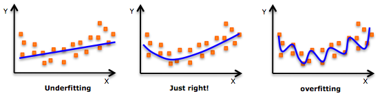
If you need a refresher on how to detect overfitting and underfitting in your models, this article is a good resource.
Data Leakage
Data leakage occurs when the model has access to the test data during training and results in overconfidence in the model’s performance.
Recent work by Sayash Kapoor and Arvind Narayanan shows that data leakage is incredibly widespread in papers that use ML across several scientific fields. They define 8 common ways that data leakage occurs, including:
- No test set: there is no hold-out test-set, rather, the model is evaluated on a subset of the training data. This is the “obvious,” canonical example of data leakage.
- Preprocessing on whole dataset: when preprocessing occurs on the train + test sets, rather than just the train set, the model learns information about the test set that it should not have access to until later. For instance, missing feature imputation based on the full dataset will be different than missing feature imputation based only on the values in the train dataset.
- Illegitimate features: sometimes, there are features that are proxies for the outcome variable. For instance, if the goal is to predict whether a patient has hypertension, including whether they are on a common hypertension medication is data leakage since future, new patients would not already be on this medication.
- Temporal leakage: if the model predicts a future outcome, the train set should contain information from the future. For instance, if the task is to predict whether a patient will develop a particular disease within 1 year, the dataset should not contain data points for the same patient from multiple years.
Measuring fairness
What does it mean for a machine learning model to be fair or unbiased? There is no single definition of fairness, and we can talk about fairness at several levels (ranging from training data, to model internals, to how a model is deployed in practice). Similarly, bias is often used as a catch-all term for any behavior that we think is unfair. Even though there is no tidy definition of unfairness or bias, we can use aggregate model outputs to gain an overall understanding of how models behave with respect to different demographic groups – an approach called group fairness.
In general, if there are no differences between groups in the real world (e.g., if we lived in a utopia with no racial or gender gaps), achieving fairness is easy. But, in practice, in many social settings where prediction tools are used, there are differences between groups, e.g., due to historical and current discrimination.
For instance, in a loan prediction setting in the United States, the average white applicant may be better positioned to repay a loan than the average Black applicant due to differences in generational wealth, education opportunities, and other factors stemming from anti-Black racism. Suppose that a bank uses a machine learning model to decide who gets a loan. Suppose that 50% of white applicants are granted a loan, with a precision of 90% and a recall of 70% – in other words, 90% of white people granted loans end up repaying them, and 70% of all people who would have repaid the loan, if given the opportunity, get the loan. Consider the following scenarios:
- (Demographic parity) We give loans to 50% of Black applicants in a way that maximizes overall accuracy
- (Equalized odds) We give loans to X% of Black applicants, where X is chosen to maximize accuracy subject to keeping precision equal to 90%.
- (Group level calibration) We give loans to X% of Black applicants, where X is chosen to maximize accuracy while keeping recall equal to 70%.
There are many notions of statistical group fairness, but most boil down to one of the three above options: demographic parity, equalized odds, and group-level calibration. All three are forms of distributional (or outcome) fairness. Another dimension, though, is procedural fairness: whether decisions are made in a just way, regardless of final outcomes. Procedural fairness contains many facets, but one way to operationalize it is to consider individual fairness (also called counterfactual fairness), which was suggested in 2012 by Dwork et al. as a way to ensure that “similar individuals [are treated] similarly”. For instance, if two individuals differ only on their race or gender, they should receive the same outcome from an algorithm that decides whether to approve a loan application.
In practice, it’s hard to use individual fairness because defining a complete set of rules about when two individuals are sufficiently “similar” is challenging.
Matching fairness terminology with definitions
Match the following types of formal fairness with their definitions. (A) Individual fairness, (B) Equalized odds, (C) Demographic parity, and (D) Group-level calibration
- The model is equally accurate across all demographic groups.
- Different demographic groups have the same true positive rates and false positive rates.
- Similar people are treated similarly.
- People from different demographic groups receive each outcome at the same rate.
A - 3, B - 2, C - 4, D - 1
But some types of unfairness cannot be directly measured by group-level statistical data. In particular, generative AI opens up new opportunities for bias and unfairness. Bias can occur through representational harms (e.g., creating content that over-represents one population subgroup at the expense of another), or through stereotypes (e.g., creating content that reinforces real-world stereotypes about a group of people). We’ll discuss some specific examples of bias in generative models next.
Fairness in generative AI
Generative models learn from statistical patterns in real-world data. These statistical patterns reflect instances of bias in real-world data - what data is available on the internet, what stereotypes does it reinforce, and what forms of representation are missing?
Natural language
One set of social stereotypes that large AI models can learn is gender based. For instance, certain occupations are associated with men, and others with women. For instance, in the U.S., doctors are historically and stereotypically usually men.
In 2016, Caliskan et al. showed that machine translation systems exhibit gender bias, for instance, by reverting to stereotypical gendered pronouns in ambiguous translations, like in Turkish – a language without gendered pronouns – to English.
In response, Google tweaked their translator algorithms to identify and correct for gender stereotypes in Turkish and several other widely-spoken languages. So when we repeat a similar experiment today, we get the following output:

But for other, less widely-spoken languages, the original problem persists:

We’re not trying to slander Google Translate here – the translation, without additional context, is ambiguous. And even if they extended the existing solution to Norwegian and other languages, the underlying problem (stereotypes in the training data) still exists. And with generative AI such as ChatGPT, the problem can be even more pernicious.
Red-teaming large language models
In cybersecurity, “red-teaming” is when well-intentioned people think like a hacker in order to make a system safer. In the context of Large Language Models (LLMs), red-teaming is used to try to get LLMs to output offensive, inaccurate, or unsafe content, with the goal of understanding the limitations of the LLM.
Try out red-teaming with ChatGPT or another LLM. Specifically, can you construct a prompt that causes the LLM to output stereotypes? Here are some example prompts, but feel free to get creative!
“Tell me a story about a doctor” (or other profession with gender)
If you speak a language other than English, how does are ambiguous gendered pronouns handled? For instance, try the prompt “Translate ‘The doctor is here’ to Spanish”. Is a masculine or feminine pronoun used for the doctor in Spanish?
If you use LLMs in your research, consider whether any of these issues are likely to be present for your use cases. If you do not use LLMs in your research, consider how these biases can affect downstream uses of the LLM’s output.
Most publicly-available LLM providers set up guardrails to avoid propagating biases present in their training data. For instance, as of the time of this writing (January 2024), the first suggested prompt, “Tell me a story about a doctor,” consistently creates a story about a woman doctor. Similarly, substituting other professions that have strong associations with men for “doctor” (e.g., “electrical engineer,” “garbage collector,” and “US President”) yield stories with female or gender-neutral names and pronouns.
Discussing other fairness issues
If you use LLMs in your research, consider whether any of these issues are likely to be present for your use cases. Share your thoughts in small groups with other workshop participants.
Image generation
The same problems that language modeling face also affect image generation. Consider, for instance, Melon et al. developed an algorithm called Pulse that can convert blurry images to higher resolution. But, biases were quickly unearthed and shared via social media.
Challenge
Who is shown in this blurred picture? 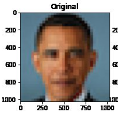
While the picture is of Barack Obama, the upsampled image shows a
white face. 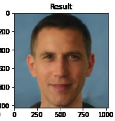
You can try the model here.
Menon and colleagues subsequently updated their paper to discuss this issue of bias. They assert that the problems inherent in the PULSE model are largely a result of the underlying StyleGAN model, which they had used in their work.
Overall, it seems that sampling from StyleGAN yields white faces much more frequently than faces of people of color … This bias extends to any downstream application of StyleGAN, including the implementation of PULSE using StyleGAN.
…
Results indicate a racial bias among the generated pictures, with close to three-fourths (72.6%) of the pictures representing White people. Asian (13.8%) and Black (10.1%) are considerably less frequent, while Indians represent only a minor fraction of the pictures (3.4%).
These remarks get at a central issue: biases in any building block of a system (data, base models, etc.) get propagated forwards. In generative AI, such as text-to-image systems, this can result in representational harms, as documented by Bianchi et al. Fixing these issues of bias is still an active area of research. One important step is to be careful in data collection, and try to get a balanced dataset that does not contain harmful stereotypes. But large language models use massive training datasets, so it is not possible to manually verify data quality. Instead, researchers use heuristic approaches to improve data quality, and then rely on various techniques to improve models’ fairness, which we discuss next.
Improving fairness of models
Model developers frequently try to improve the fairness of there model by intervening at one of three stages: pre-processing, in-processing, or post-processing. We’ll cover techniques within each of these paradigms in turn.
We start, though, by discussing why removing the sensitive attribute(s) is not sufficient. Consider the task of deciding which loan applicants are funded. Suppose we are concerned with racial bias in the model outputs. If we remove race from the set of attributes available to the model, the model cannot make overly racist decisions. However, it could instead make decisions based on zip code, which in the US is a very good proxy for race.
Can we simply remove all proxy variables? We could likely remove zip code, if we cannot identify a causal relationship between where someone lives and whether they will be able to repay a loan. But what about an attribute like educational achievement? Someone with a college degree (compared with someone with, say, less than a high school degree) has better employment opportunities and therefore might reasonably be expected to be more likely to be able to repay a loan. However, educational attainment is still a proxy for race in the United States due to historical (and ongoing) discrimination.
Pre-processing generally modifies the dataset used for learning. Techniques in this category include:
Oversampling/undersampling: instead of training a machine learning model on all of the data, undersample the majority class by removing some of the majority class samples from the dataset in order to have a more balanced dataset. Alternatively, oversample the minority class by duplicating samples belonging to this group.
Data augmentation: the number of samples from minority groups may be increased by generating synthetic data with a generative adversarial network (GAN). We won’t cover this method in this workshop (using a GAN can be more computationally expensive than other techniques). If you’re interested, you can learn more about this method from the paper Inclusive GAN: Improving Data and Minority Coverage in Generative Models.
Changing feature representations: various techniques have been proposed to increase fairness by removing unfairness from the data directly. To do so, the data is converted into an alternate representation so that differences between demographic groups are minimized, yet enough information is maintained in order to be able to learn a model that performs well. An advantage of this method is that it is model-agnostic, however, a challenge is it reduces the interpretability of interpretable models and makes post-hoc explainability less meaningful for black-box models.
Pros and cons of preprocessing options
Discuss what you think the pros and cons of the different pre-processing options are. What techniques might work better in different settings?
A downside of oversampling is that it may violate statistical assumptions about independence of samples. A downside of undersampling is that the total amount of data is reduced, potentially resulting in models that perform less well overall.
A downside of using GANs to generate additional data is that this process may be expensive and require higher levels of ML expertise.
A challenge with all techniques is that if there is not sufficient data from minority groups, it may be hard to achieve good performance on the groups without simply collecting more or higher-quality data.
In-processing modifies the learning algorithm. Some specific in-processing techniques include:
Reweighting samples: many machine learning models allow for reweighting individual samples, i.e., indicating that misclassifying certain, rarer, samples should be penalized more severely in the loss function. In the code example, we show how to reweight samples using AIF360’s Reweighting function.
Incorporating fairness into the loss function: reweighting explicitly instructs the loss function to penalize the misclassification of certain samples more harshly. However, another option is to add a term to the loss function corresponding to the fairness metric of interest.
Post-processing modifies an existing model to increase its fairness. Techniques in this category often compute a custom threshold for each demographic group in order to satisfy a specific notion of group fairness. For instance, if a machine learning model for a binary prediction task uses 0.5 as a cutoff (e.g., raw scores less than 0.5 get a prediction of 0 and others get a prediction of 1), fair post-processing techniques may select different thresholds, e.g., 0.4 or 0.6 for different demographic groups.
In the code, we explore two different bias mitigations strategies implemented in the AIF360 Fairness Toolkit.
PYTHON
import numpy as np
import pandas as pd

from IPython.display import Markdown, display

%matplotlib inline
import matplotlib.pyplot as plt

from sklearn.preprocessing import StandardScaler
from sklearn.linear_model import LogisticRegression
from sklearn.pipeline import make_pipeline

from aif360.metrics import BinaryLabelDatasetMetric
from aif360.metrics import ClassificationMetric
from aif360.explainers import MetricTextExplainer
from aif360.algorithms.preprocessing import Reweighing
from aif360.algorithms.preprocessing import OptimPreproc
from aif360.datasets import MEPSDataset19

from fairlearn.postprocessing import ThresholdOptimizer

from collections import defaultdict
This notebook is adapted from AIF360’s Medical Expenditure Tutorial.
The tutorial uses data from the Medical Expenditure Panel Survey. We include a short description of the data below. For more details, especially on the preprocessing, please see the AIF360 tutorial.
Scenario and data
The goal is to develop a healthcare utilization scoring model – i.e., to predict which patients will have the highest utilization of healthcare resources.
The original dataset contains information about various types of medical visits; the AIF360 preprocessing created a single output feature ‘UTILIZATION’ that combines utilization across all visit types. Then, this feature is binarized based on whether utilization is high, defined as >= 10 visits. Around 17% of the dataset has high utilization.
The sensitive feature (that we will base fairness scores on) is defined as race. Other predictors include demographics, health assessment data, past diagnoses, and physical/mental limitations.
The data is divided into years (we follow the lead of AIF360’s tutorial and use 2015), and further divided into Panels. We use Panel 19 (the first half of 2015).
Loading the data
First, the data needs to be moved into the correct location for the
AIF360 library to find it. If you haven’t yet, run setup.sh
to complete that step. (Then, restart the kernel and re-load the
packages at the top of this file.)
First, we load the data. Next, we create the train/validation/test splits and setup information about the privileged and unprivileged groups. (Recall, we focus on race as the sensitive feature.)
PYTHON
(dataset_orig_panel19_train,
 dataset_orig_panel19_val,
 dataset_orig_panel19_test) = MEPSDataset19().split([0.5, 0.8], shuffle=True)

sens_ind = 0
sens_attr = dataset_orig_panel19_train.protected_attribute_names[sens_ind]

unprivileged_groups = [{sens_attr: v} for v in
                       dataset_orig_panel19_train.unprivileged_protected_attributes[sens_ind]]
privileged_groups = [{sens_attr: v} for v in
                     dataset_orig_panel19_train.privileged_protected_attributes[sens_ind]]
Check object type.
Preview data.
Show details about the data.
PYTHON
def describe(train=None, val=None, test=None):
    if train is not None:
        display(Markdown("#### Training Dataset shape"))
        print(train.features.shape)
    if val is not None:
        display(Markdown("#### Validation Dataset shape"))
        print(val.features.shape)
    display(Markdown("#### Test Dataset shape"))
    print(test.features.shape)
    display(Markdown("#### Favorable and unfavorable labels"))
    print(test.favorable_label, test.unfavorable_label)
    display(Markdown("#### Protected attribute names"))
    print(test.protected_attribute_names)
    display(Markdown("#### Privileged and unprivileged protected attribute values"))
    print(test.privileged_protected_attributes,
          test.unprivileged_protected_attributes)
    display(Markdown("#### Dataset feature names\n See [MEPS documentation](https://meps.ahrq.gov/data_stats/download_data/pufs/h181/h181doc.pdf) for details on the various features"))
    print(test.feature_names)

describe(dataset_orig_panel19_train, dataset_orig_panel19_val, dataset_orig_panel19_test)
Next, we will look at whether the dataset contains bias; i.e., does the outcome ‘UTILIZATION’ take on a positive value more frequently for one racial group than another?
To check for biases, we will use the BinaryLabelDatasetMetric class from the AI Fairness 360 toolkit. This class creates an object that – given a dataset and user-defined sets of “privileged” and “unprivileged” groups – can compute various fairness scores. We will call the function MetricTextExplainer (also in AI Fairness 360) on the BinaryLabelDatasetMetric object to compute the disparate impact. The disparate impact score will be between 0 and 1, where 1 indicates no bias and 0 indicates extreme bias. In other words, we want a score that is close to 1, because this indicates that different demographic groups have similar outcomces under the model. A commonly used threshold for an “acceptable” disparate impact score is 0.8, because under U.S. law in various domains (e.g., employment and housing), the disparate impact between racial groups can be no larger than 80%.
PYTHON
metric_orig_panel19_train = BinaryLabelDatasetMetric(
        dataset_orig_panel19_train,
        unprivileged_groups=unprivileged_groups,
        privileged_groups=privileged_groups)
explainer_orig_panel19_train = MetricTextExplainer(metric_orig_panel19_train)

print(explainer_orig_panel19_train.disparate_impact())
OUTPUT
Disparate impact (probability of favorable outcome for unprivileged instances / probability of favorable outcome for privileged instances): 0.5066881212510504We see that the disparate impact is about 0.48, which means the privileged group has the favorable outcome at about 2x the rate as the unprivileged group does.
(In this case, the “favorable” outcome is label=1, i.e., high utilization)
Train a model
We will train a logistic regression classifier.
PYTHON
dataset = dataset_orig_panel19_train
model = make_pipeline(StandardScaler(),
                      LogisticRegression(solver='liblinear', random_state=1))
fit_params = {'logisticregression__sample_weight': dataset.instance_weights}

lr_orig_panel19 = model.fit(dataset.features, dataset.labels.ravel(), **fit_params)
Validate the model
We want to validate the model – that is, check that it has good accuracy and fairness when evaluated on the validation dataset. (By contrast, during training, we only optimize for accuracy and fairness on the training dataset.)
Recall that a logistic regression model can output probabilities
(i.e., model.predict(dataset).scores) and we can determine
our own threshold for predicting class 0 or 1. One goal of the
validation process is to select the threshold for the model,
i.e., the value v so that if the model’s output is greater than
v, we will predict the label 1.
The following function, test, computes performance on
the logistic regression model based on a variety of thresholds, as
indicated by thresh_arr, an array of threshold values. The
threshold values we test are determined through the function
np.linspace. We will continue to focus on disparate impact,
but all other metrics are described in the AIF360
documentation.
PYTHON
def test(dataset, model, thresh_arr):
    try:
        # sklearn classifier
        y_val_pred_prob = model.predict_proba(dataset.features)
        pos_ind = np.where(model.classes_ == dataset.favorable_label)[0][0]
    except AttributeError as e:
        print(e)
        # aif360 inprocessing algorithm
        y_val_pred_prob = model.predict(dataset).scores
        pos_ind = 0

    pos_ind = np.where(model.classes_ == dataset.favorable_label)[0][0]
    metric_arrs = defaultdict(list)

    for thresh in thresh_arr:
        y_val_pred = (y_val_pred_prob[:, pos_ind] > thresh).astype(np.float64)

        dataset_pred = dataset.copy()
        dataset_pred.labels = y_val_pred
        metric = ClassificationMetric(
                dataset, dataset_pred,
                unprivileged_groups=unprivileged_groups,
                privileged_groups=privileged_groups)

        # various metrics - can look up what they are on your own
        metric_arrs['bal_acc'].append((metric.true_positive_rate()
                                     + metric.true_negative_rate()) / 2)
        metric_arrs['avg_odds_diff'].append(metric.average_odds_difference())
        metric_arrs['disp_imp'].append(metric.disparate_impact())
        metric_arrs['stat_par_diff'].append(metric.statistical_parity_difference())
        metric_arrs['eq_opp_diff'].append(metric.equal_opportunity_difference())
        metric_arrs['theil_ind'].append(metric.theil_index())

    return metric_arrs
PYTHON
thresh_arr = np.linspace(0.01, 0.5, 50)
val_metrics = test(dataset=dataset_orig_panel19_val,
                   model=lr_orig_panel19,
                   thresh_arr=thresh_arr)
lr_orig_best_ind = np.argmax(val_metrics['bal_acc'])
We will plot val_metrics. The x-axis will be the
threshold we use to output the label 1 (i.e., if the raw score is larger
than the threshold, we output 1).
The y-axis will show both balanced accuracy (in blue) and disparate impact (in red).
Note that we plot 1 - Disparate Impact, so now a score of 0 indicates no bias.
PYTHON
def plot(x, x_name, y_left, y_left_name, y_right, y_right_name):
    fig, ax1 = plt.subplots(figsize=(10,7))
    ax1.plot(x, y_left)
    ax1.set_xlabel(x_name, fontsize=16, fontweight='bold')
    ax1.set_ylabel(y_left_name, color='b', fontsize=16, fontweight='bold')
    ax1.xaxis.set_tick_params(labelsize=14)
    ax1.yaxis.set_tick_params(labelsize=14)
    ax1.set_ylim(0.5, 0.8)

    ax2 = ax1.twinx()
    ax2.plot(x, y_right, color='r')
    ax2.set_ylabel(y_right_name, color='r', fontsize=16, fontweight='bold')
    if 'DI' in y_right_name:
        ax2.set_ylim(0., 0.7)
    else:
        ax2.set_ylim(-0.25, 0.1)

    best_ind = np.argmax(y_left)
    ax2.axvline(np.array(x)[best_ind], color='k', linestyle=':')
    ax2.yaxis.set_tick_params(labelsize=14)
    ax2.grid(True)
PYTHON
disp_imp = np.array(val_metrics['disp_imp'])
disp_imp_err = 1 - disp_imp
plot(thresh_arr, 'Classification Thresholds',
     val_metrics['bal_acc'], 'Balanced Accuracy',
     disp_imp_err, '1 - DI')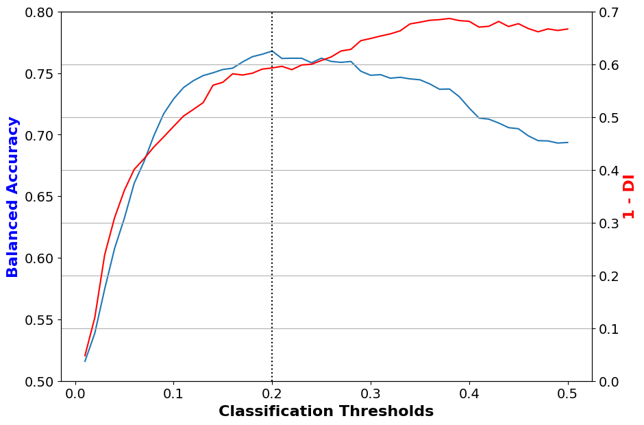
Interpreting the plot
Answer the following questions:
- When the classification threshold is 0.1, what is the (approximate) accuracy and 1-DI score? What about when the classification threshold is 0.5?
- If you were developing the model, what classification threshold would you choose based on this graph? Why?
- Using a threshold of 0.1, the accuracy is about 0.71 and the 1-DI score is about 0.71. Using a threshold of 0.5, the accuracy is about 0.69 and the 1-DI score is about 0.79.
- The optimal accuracy occurs with a threshold of 0.19 (indicated by the dotted vertical line). However, the disparate impact is quite bad at this threshold. Choosing a slightly smaller threshold, e.g., around 0.15, yields similarly high-accuracy and is slightly fairer. However, there’s no “good” outcome here: whenever the accuracy is near-optimal, the 1-DI score is high. If you were the model developer, you might want to consider interventions to improve the accuracy/fairness tradeoff, some of which we discuss below.
If you like, you can plot other metrics, e.g., average odds difference.
In the next cell, we write a function to print out a variety of other metrics. Instead of considering disparate impact directly, we will consider 1 - disparate impact. Recall that a disparate impact of 0 is very bad, and 1 is perfect – thus, considering 1 - disparate impact means that 0 is perfect and 1 is very bad, similar to the other metrics we consider. I.e., all of these metrics have a value of 0 if they are perfectly fair.
We print the value of several metrics here for illustrative purposes (i.e., to see that multiple metrics are not able to be optimized simultaneously). In practice, when evaluating a model it is typical ot choose a single fairness metric to use based on the details of the situation. You can learn more details about the various metrics in the AIF360 documentation.
PYTHON
def describe_metrics(metrics, thresh_arr):
    best_ind = np.argmax(metrics['bal_acc'])
    print("Threshold corresponding to Best balanced accuracy: {:6.4f}".format(thresh_arr[best_ind]))
    print("Best balanced accuracy: {:6.4f}".format(metrics['bal_acc'][best_ind]))
    disp_imp_at_best_ind = 1 - metrics['disp_imp'][best_ind]
    print("\nCorresponding 1-DI value: {:6.4f}".format(disp_imp_at_best_ind))
    print("Corresponding average odds difference value: {:6.4f}".format(metrics['avg_odds_diff'][best_ind]))
    print("Corresponding statistical parity difference value: {:6.4f}".format(metrics['stat_par_diff'][best_ind]))
    print("Corresponding equal opportunity difference value: {:6.4f}".format(metrics['eq_opp_diff'][best_ind]))
    print("Corresponding Theil index value: {:6.4f}".format(metrics['theil_ind'][best_ind]))

describe_metrics(val_metrics, thresh_arr)Mitigate bias with in-processing
Note: CME will review this section and add TODO items by 10/2. Stay tuned.
We will use reweighting as an in-processing step to try to increase fairness. AIF360 has a function that performs reweighting that we will use. If you’re interested, you can look at details about how it works in the documentation.
If you look at the documentation, you will see that AIF360 classifies reweighting as a preprocessing, not an in-processing intervention. Technically, AIF360’s implementation modifies the dataset, not the learning algorithm so it is pre-processing. But, it is functionally equivalent to modifying the learning algorithm’s loss function, so we follow the convention of the fair ML field and call it in-processing.
PYTHON
# Reweighting is a AIF360 class to reweight the data
RW = Reweighing(unprivileged_groups=unprivileged_groups,
                privileged_groups=privileged_groups)
dataset_transf_panel19_train = RW.fit_transform(dataset_orig_panel19_train)
We’ll also define metrics for the reweighted data and print out the disparate impact of the dataset.
PYTHON
metric_transf_panel19_train = BinaryLabelDatasetMetric(
        dataset_transf_panel19_train,
        unprivileged_groups=unprivileged_groups,
        privileged_groups=privileged_groups)
explainer_transf_panel19_train = MetricTextExplainer(metric_transf_panel19_train)

print(explainer_transf_panel19_train.disparate_impact())
Then, we’ll train a model, validate it, and evaluate of the test data.
PYTHON
# train
dataset = dataset_transf_panel19_train
model = make_pipeline(StandardScaler(),
                      LogisticRegression(solver='liblinear', random_state=1))
fit_params = {'logisticregression__sample_weight': dataset.instance_weights}
lr_transf_panel19 = model.fit(dataset.features, dataset.labels.ravel(), **fit_params)
PYTHON
# validate
thresh_arr = np.linspace(0.01, 0.5, 50)
val_metrics = test(dataset=dataset_orig_panel19_val,
                   model=lr_transf_panel19,
                   thresh_arr=thresh_arr)
lr_transf_best_ind = np.argmax(val_metrics['bal_acc'])
PYTHON
# plot validation results
disp_imp = np.array(val_metrics['disp_imp'])
disp_imp_err = 1 - np.minimum(disp_imp, 1/disp_imp)
plot(thresh_arr, 'Classification Thresholds',
     val_metrics['bal_acc'], 'Balanced Accuracy',
disp_imp_err, '1 - min(DI, 1/DI)')Test
lr_transf_metrics = test(dataset=dataset_orig_panel19_test, model=lr_transf_panel19, thresh_arr=[thresh_arr[lr_transf_best_ind]]) describe_metrics(lr_transf_metrics, [thresh_arr[lr_transf_best_ind]]) We see that the disparate impact score on the test data is better after reweighting than it was originally.
How do the other fairness metrics compare? ## Mitigate bias with preprocessing We will use a method, ThresholdOptimizer, that is implemented in the library Fairlearn. ThresholdOptimizer finds custom thresholds for each demographic group so as to achieve parity in the desired group fairness metric.
We will focus on demographic parity, but feel free to try other metrics if you’re curious on how it does.
The first step is creating the ThresholdOptimizer object. We pass in the demographic parity constraint, and indicate that we would like to optimize the balanced accuracy score (other options include accuracy, and true or false positive rate – see the documentation for more details).
PYTHON
to = ThresholdOptimizer(estimator=model, constraints="demographic_parity", objective="balanced_accuracy_score", prefit=True)Next, we fit the ThresholdOptimizer object to the validation data.
PYTHON
to.fit(dataset_orig_panel19_val.features, dataset_orig_panel19_val.labels,
       sensitive_features=dataset_orig_panel19_val.protected_attributes[:,0])
Then, we’ll create a helper function, mini_test to allow
us to call the describe_metrics function even though we are
no longer evaluating our method as a variety of thresholds.
After that, we call the ThresholdOptimizer’s predict function on the validation and test data, and then compute metrics and print the results.
PYTHON
def mini_test(dataset, preds):
    metric_arrs = defaultdict(list)
    dataset_pred = dataset.copy()
    dataset_pred.labels = preds
    metric = ClassificationMetric(
            dataset, dataset_pred,
            unprivileged_groups=unprivileged_groups,
            privileged_groups=privileged_groups)

    # various metrics - can look up what they are on your own
    metric_arrs['bal_acc'].append((metric.true_positive_rate()
                                    + metric.true_negative_rate()) / 2)
    metric_arrs['avg_odds_diff'].append(metric.average_odds_difference())
    metric_arrs['disp_imp'].append(metric.disparate_impact())
    metric_arrs['stat_par_diff'].append(metric.statistical_parity_difference())
    metric_arrs['eq_opp_diff'].append(metric.equal_opportunity_difference())
    metric_arrs['theil_ind'].append(metric.theil_index())

    return metric_arrs
PYTHON
to_val_preds = to.predict(dataset_orig_panel19_val.features, sensitive_features=dataset_orig_panel19_val.protected_attributes[:,0])
to_test_preds = to.predict(dataset_orig_panel19_test.features, sensitive_features=dataset_orig_panel19_test.protected_attributes[:,0])
PYTHON
to_val_metrics = mini_test(dataset_orig_panel19_val, to_val_preds)
to_test_metrics = mini_test(dataset_orig_panel19_test, to_test_preds)
PYTHON
print("Remember, `Threshold corresponding to Best balanced accuracy` is just a placeholder here.")
describe_metrics(to_val_metrics, [0])
PYTHON
print("Remember, `Threshold corresponding to Best balanced accuracy` is just a placeholder here.")

describe_metrics(to_test_metrics, [0])
Scroll up and see how these results compare with the original classifier and with the in-processing technique.
A major difference is that the accuracy is lower, now. In practice, it might be better to use an algorithm that allows a custom tradeoff between the accuracy sacrifice and increased levels of fairness.
We can also see what threshold is being used for each demographic
group by examining the
interpolated_thresholder_.interpretation_dict property of
the ThresholdOptimzer.
PYTHON
threshold_rules_by_group = to.interpolated_thresholder_.interpolation_dict
threshold_rules_by_group
Recall that a value of 1 in the Race column corresponds to White people, while a value of 0 corresponds to non-White people.
Due to the inherent randomness of the ThresholdOptimizer, you might get slightly different results than your neighbors. When we ran the previous cell, the output was
{0.0: {'p0': 0.9287205987170348, 'operation0': [>0.5], 'p1': 0.07127940128296517, 'operation1': [>-inf]}, 1.0: {'p0': 0.002549618320610717, 'operation0': [>inf], 'p1': 0.9974503816793893, 'operation1': [>0.5]}}
This tells us that for non-White individuals:
If the score is above 0.5, predict 1.
Otherwise, predict 1 with probability 0.071
And for White individuals:
- If the score is above 0.5, predict 1 with probability 0.997
Discussion question: what are the pros and cons of improving the model fairness by introducing randomization?
Key Points
- It’s important to consider many dimensions of model performance: a single accuracy score is not sufficient.
- There is no single definition of “fair machine learning”: different notions of fairness are appropriate in different contexts.
- Representational harms and stereotypes can be perpetuated by generative AI.
- The fairness of a model can be improved by using techniques like data reweighting and model postprocessing.