Efficient Computing in Julia: All in One View

Last updated on 2025-02-10 | Edit this page

Overview

Questions

Why should I use Julia?
How do I get started with Julia?

Objectives

Start a REPL
Run lines from VS Code

Overview of the Workshop

It is not feasible to teach all of Julia in just two days. We’ll try to get you on your journey with Julia by showing lots of real world examples. Meanwhile, you’ll be Roughly:

(3h) Get you started with Julia by simulating gravity: the three body problem. You’ll get familiar with the basic syntax of Julia and the little nooks and crannies that set this language appart from Python or MATLAB.
(3h) Learn to work with Julia’s packaging system and best practices.
(4h) Benchmarking, profiling, type stability and allocations. We will work with many different examples here. You’ll learn the most important tools and concepts that matter when you want to write Julia code that runs efficiently.
(2h) Parallel and GPU programming: computing the Julia fractal.

Some of the examples may be a bit hard to grasp. For example, we’ll see a very difficult to understand algorithm to compute $\pi$. In these cases we’ll treat the given code as black boxes that we can poke at. The power of a good computer program is often that we don’t need to know everything to be able to work with it.

Why Julia

Most of the participants will be coming from Python, MATLAB or a lower level language like C/C++ or Fortran. Why should you be interested in learning Julia?

Performance and usability

Julia promises:

Native performance: close to or sometimes even exceeding C++ or Fortran.
Solve the multiple language issue: one language for everything (including GPU).
As easy to get into as Python or R.
Designed for parallel computing.

These promises seem tantalizing and are in part what draws people to Julia, but in practice getting into Julia and writing performant code are two different things. Julia has its own idiosyncrasies that need to be understood to really squeeze every erg of performance out of your system.

Julia obtains its performance from being a just-in-time (JIT) compiler, on top of the LLVM compiler stack (similar to how Python’s Numba operates).

Language intrinsics

Next to being performant, it turns out that Julia is a very nice language that does some things a bit different from what you may be used to:

First-class arrays and Broadcasting: arrays, slicing and operating on arrays have dedicated syntax, similar to MATLAB.
Multiple dispatch: Julia functions can be specialized on the entire call signature (not just its first argument like in Object Oriented Programming).
Macros and Meta-programming: The just-in-time nature of the Julia compiler exposes a wide range of meta-programming capabilities, ranging from small macros to enhance the expressibility of the language to full-on code generation.

Meta-programming, while very powerful, is also very easy to abuse, often leading to unreadable non-idiomatic code. So tread with care! We’ll see some examples where macros are indispensable though, and the SciML stack relies deeply on on-the-fly code-generation.

Discussion

Why are you interested in Julia? What is your current go-to for efficient computing?

Recommended materials

If you want to learn more about computer programming in general, a great place to start is Structure and Interpretation of Computer Programs, including the Lectures on Youtube. These are old but wonderful and really teach some wisdom around designing complex software systems. Also, this might cure any latent adiction to object oriented programming.

If you want to learn about efficient programming in Julia, check out Parallel Computing and Scientific Machine Learning. These go in much more detail than we can do in this lecture.

The materials in this lesson are aimed somewhere in between SICP and PCSML. We’ll look at real scientific examples to dive into computational concepts.

Running Julia

When working in Julia it is very common to do so from the REPL (Read-Eval-Print Loop). Please open the Julia REPL on your system

$ julia

OUTPUT

               _
   _       _ _(_)_     |  Documentation: https://docs.julialang.org
  (_)     | (_) (_)    |
   _ _   _| |_  __ _   |  Type "?" for help, "]?" for Pkg help.
  | | | | | | |/ _` |  |
  | | |_| | | | (_| |  |  Version 1.10.3 (2024-04-30)
 _/ |\__'_|_|_|\__'_|  |  Official https://julialang.org/ release
|__/                   |

julia>

The REPL needs a small introduction since it has several modes.

Key	Prompt	Mode
None	`julia>`	Standard Julia input.
`]`	`pkg>`	Pkg mode. Commands entered here are functions in the `Pkg` module.
`;`	`shell>`	Shell mode.
`?`	`help?>`	Help mode. Type the name of any entity to look up its documentation.

To switch back to the standard Julia input from another mode, press Ctrl+C

Play with the REPL (5min)

Pkg mode has a help command to help you along. Find out what the add command does.
Check the contents of the folder in which you are running your REPL (ls on Unix, dir on Windows).
Find out what the print method does in Julia.

Show me the solution

]help add, the add command installs packages
;ls
?print

Callout

Please take a look at the Julia documentation now at https://docs.julialang.org/en/v1/.

Pluto

Pluto is the notebook environment from which we will teach much of this workshop. We can run it from the Julia REPL.

OUTPUT

pkg> add Pluto
... quite a bit of output ...

julia> using Pluto

julia> Pluto.run()
[ Info: Loading...
┌ Info:
└ Opening http://localhost:1235/?secret=xyzxyzxyz in your default browser... ~ have fun!
┌ Info:
│ Press Ctrl+C in this terminal to stop Pluto
└

VS Code

VS Code is the editor for which Julia has the best support. We’ll be needing to run Julia in multiple threads later on, so we’ll set some arguments for the REPL in settings.json (press Ctrl+Shift+P and search for Open User Settings (JSON)).

JSON

{
    ...
    "julia.additionalArgs": [ 
        "-t", "4"
    ]
}

Now when you start a new REPL (Ctrl+Shift+P, search “Julia REPL”), you can query the number of threads available:

JULIA

Threads.nthreads()

Julia as a calculator (5min)

Try to play around in the VS Code REPL to use Julia as a calculator.

What do you find is the operator for exponentiation?
How do you assign a variable?
What happens when you divide any two integers? Use the typeof function to inspect the type of the result. Can you figure out how to integer division (search the documentation!)?
What happens in Pluto when you change a variable that is depended upon?

Show me the solution

In Julia exponentiation is ^.
Just like you’re used to x = 3.
The / operator always returns a floating point value. To get to integer division, we want the ÷ operator, which can be typed using \div and then press TAB. Or you can use the equivalent div function.
Pluto updates all dependent computations automatically. This is known as a reactive notebook.

Key Points

In Julia, the REPL is much more important than in some other languages.
Pluto is a reactive environment
VS Code has the best editor integration for Julia

Activate the Workshop Environment

For this workshop, we prepared an environment. Press ] in the REPL to activate Pkg mode. Make sure that you are in the path where you prepared your environment (see Setup Instructions).

(v1.11) pkg> activate .
(EfficientJulia) pkg>

Alternatively, check the little “Julia env” message at the bottom of VS Code, and make sure that the correct environment is there.

You should now be able to generate a plot using GLMakie (that one dependency that made you wait)

JULIA

using GLMakie
x = -3.0:0.1:3.0
z = sinc.(sqrt.(x.^2 .+ x'.^2))
surface(x, x, z, alpha=0.5)
wireframe!(x, x, z, color=:black, linewidth=0.5)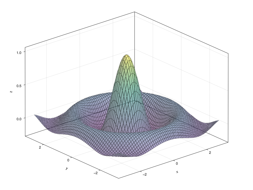

Figure code

To create the above figure:

JULIA

#| classes: ["task"]
#| creates: episodes/fig/getting-started-makie.png
#| collect: figures

module Script
using GLMakie

function main()
    x = -3.0:0.1:3.0
    z = sinc.(sqrt.(x.^2 .+ x'.^2))

    fig = Figure(size=(1024, 768))
    ax = Axis3(fig[1,1])
    surface!(ax, x, x, z, alpha=0.5)
    wireframe!(ax, x, x, z, color=:black, linewidth=0.5)
    save("episodes/fig/getting-started-makie.png", fig)
end
end

Script.main()

Content from Introduction to Julia

Last updated on 2025-02-10 | Edit this page

Overview

Questions

How do I write elementary programs in Julia?
What are the differences with Python/MATLAB/R?

Objectives

functions
loops
conditionals
scoping

Unfortunately, it lies outside the scope of this workshop to give an introduction to the full Julia language. Instead, we’ll briefly show the basic syntax, and then focus on some key differences with other popular languages.

About Julia

These are some words that we will write down: never forget.

A just-in-time compiled, dynamically typed language
multiple dispatch
expression based syntax
rich macro system

Oddities for Pythonistas:

1-based indexing
lexical scoping

Better well stolen … Always ask when learning a new language: what are the primitives, the means of combination and the means of abstraction. Many languages are very similar in these regards, so we’ll look at things that are different:

What	Procedures	Data
primitives	standard library	(numbers, strings, etc.) arrays, symbols, channels
means of combination	(`for`, `if` etc.) broadcasting, `do`	tuples, `struct`, expressions
means of abstraction	functions, dispatch, macros (no classes!)	`abstract type`, generics

Eval

How is Julia evaluated? Types only instantiate at run-time, triggering the compile time specialization of untyped functions.

Julia can be “easy”, because the user doesn’t have to tinker with types.
Julia can be “fast”, as soon as the compiler knows all the types.

When a function is called with a hitherto new type signature, compilation is triggered. Julia’s biggest means of abstraction: multiple dispatch is only an emergent property of this evaluation strategy.

Julia has a heritage from functional programming languages (nowadays well hidden not to scare people). What we get from this:

expression based syntax: everything is an expression, meaning it reduces to a value
a rich macro system: we can extend the language itself to suit our needs (not covered in this workshop)

Julia is designed to replace MATLAB:

high degree of built-in support for multi-dimensional arrays and linear algebra
ecosystem of libraries around numeric modelling

Julia is designed to replace Fortran:

high performance
accelerate using Threads or through the GPU interfaces
scalable through Distributed or MPI

Julia is designed to replace Conda:

quality package system with pre-compiled binary libraries for system dependencies
highly reproducible
easy to use on HPC facilities

Julia is not (some people might get angry for this):

a suitable scripting language
a systems programming language like C or Rust (imagine waiting for ls to compile every time you run it)
replacing either C or Python anytime soon

Functions

Functions are declared with the function keyword. The block or function body is ended with end. All blocks in Julia end with end.

JULIA

const G = 6.6743e-11

function gravitational_force(m1, m2, r)
  return G * m1 * m2 / r^2
end

There is a shorter syntax for functions that is useful for one-liners:

JULIA

gravitational_force(m1, m2, r) = G * m1 * m2 / r^2

Anonymous functions (or lambdas)

Julia inherits a lot of concepts from functional programming. There are two ways to define anonymous functions:

JULIA

F_g = function(m1, m2, r)
  return G * m1 * m2 / r^2
end

And a shorter syntax,

JULIA

F_g = (m1, m2, r) -> G * m1 * m2 / r^2

Higher order functions

Use the map function in combination with an anonymous function to compute the squares of the first ten integers (use 1:10 to create that range).

Show me the solution

Read the documentation of map using the ? help mode in the REPL.

JULIA

map(x -> x^2, 1:10)

In fact, we’ll see that map is not often used, since Julia has many better ways to express mapping operations of this kind.

If statements, for loops

Here’s another function that’s a little more involved.

JULIA

function is_prime(x)
  if x < 2
    return false
  end

  for i = 2:isqrt(x)
    if x % i == 0
      return false
    end
  end

  return true
end

Ranges

The for loop iterates over the range 2:isqrt(x). We’ll see that Julia indexes sequences starting at integer value 1. This usually implies that ranges are given inclusive on both ends: for example, collect(3:6) evaluates to [3, 4, 5, 6].

More on for-loops

Loop iterations can be skipped using continue, or broken with break, identical to C or Python.

Challenge

The i == j && continue is a short-cut notation for

JULIA

if i == j
	continue
end

We could also have written i != j || continue.

In general, the || and && operators can be chained to check increasingly stringent tests. For example:

JULIA

inbounds(Bool, i, data) && data[i] < 10 && return 3*data[i]

Here, the second condition can only be evaluated if the first one was true.

Rewrite the is_prime function using this notation.

Show me the solution

JULIA

function is_prime(x)
    x < 2 && return false
    for i = 2:isqrt(x)
        x % i == 0 && return false
    end
    return true
end

is_prime(42)
is_prime(43)

Return statement

In Julia, the return statement is not always strictly necessary. Every statement is an expression, meaning that it has a value. The value of a compound block is simply that of its last expression. In the above function however, we have a non-local return: once we find a divider for a number, we know the number is not prime, and we don’t need to check any further.

Many people find it more readable however, to always have an explicit return.

The fact that the return statement is optional for normal function exit is part of a larger philosophy: everything is an expression.

Lexical scoping

Julia is lexically scoped. This means that variables do not outlive the block that they’re defined in. In a nutshell, this means the following:

JULIA

let s = 42
  println(s)

  for s = 1:5
    println(s)
  end

  println(s)
end

OUTPUT

In effect, the variable s inside the for-loop is said to shadow the outer definition. Here, we also see a first example of a let binding, creating a scope for some temporary variables to live in.

Loops and conditionals

Write a loop that prints out all primes below 100.

Show me the solution

JULIA

for i in 1:100
  if is_prime(i)
    println(i)
  end
end

If you like to collect those into a vector, try the following:

JULIA

1:100 |> filter(is_prime) |> collect

Macros

Julia has macros. These are invocations that change the behaviour of a given piece of code. In effect, arguments of a macro are syntactic forms that can be rewritten by the macro. These can reduce the amount of code you need to write to express certain concepts. You can recognize macro calls by the @ sign in front of them.

JULIA

@assert true "This will always pass"
@assert false "Oh, noes!"
@macroexpand @assert false "Oh, noes!"

We will explain some macro’s as they are used. We won’t get into writing macros ourselves. They can be incredibly useful, but should also come with a warning: overuse of macros can make your code non-idiomatic and therefore harder to read. Also macro-heavy frameworks tend to be harder to debug, and often lack in composability.

Arrays and broadcasting

Julia has built-in support for multi-dimensional arrays. Any function that can be applied to single values, can also be applied to entire arrays using the concept of broadcasting.

JULIA

x = -2π:0.01:2π
y = sin.(x)

Notice that the broadcasting mechanism works transparently over ranges as well as arrays. We can sequence broadcasted operations:

JULIA

y = sin.(x) ./ x

The compiler will fuse chained broadcasting operations into a single loop. We could spend half the workshop on getting good at array based operations, but we won’t. Instead, we refer to the Julia documentation on arrays. During the rest of the workshop you will be exposed to array based computation here and there.

Key Points

Julia has if-else, for, while, function and module blocks that are not dissimilar from other languages.
Blocks are all ended with end.
Always enclose code in functions because functions are compiled
Don’t use global mutable variables
Julia variables are not visible outside the block in which they’re defined (unlike Python).

Content from Types and Dispatch

Last updated on 2025-02-10 | Edit this page

Overview

Questions

How does Julia deal with types?
Can I do Object Oriented Programming?
People keep talking about multiple dispatch. What makes it so special?

Objectives

dispatch
structs
abstract types

Julia is a dynamically typed language. Nevertheless, we will see that knowing where and where not to annotate types in your program is crucial for managing performance.

In Julia there are two reasons for using the type system:

structuring your data by declaring a struct
dispatching methods based on their argument types

Inspection

You may inspect the dynamic type of a variable or expression using the typeof function. For instance:

JULIA

typeof(3)

OUTPUT

Int64

JULIA

typeof("hello")

OUTPUT

String

(plenary) Types of floats

Check the type of the following values:

3
3.14
6.62607015e-34
6.6743f-11
6e0 * 7f0

Show me the solution

Int64
Float64
Float64
Float32
Float64

Structures

JULIA

struct Point2
  x::Float64
  y::Float64
end

JULIA

let p = Point2(1, 3)
  println("Point at $(p.x), $(p.y)")
end

Methods

JULIA

dot(a::Point2, b::Point2) = a.x*b.x + a.y*b.y

3D Point

Create a structure that represents a point in 3D space and implement the dot product for it.

Show me the solution

JULIA

struct Point3
  x::Float64
  y::Float64
  z::Float64
end

dot(a::Point3, b::Point3) = a.x*b.x + a.y*b.y + a.z*b.z

Multiple dispatch (function overloading)

JULIA

Base.:+(a::Point2, b::Point2) = Point2(a.x+b.x, a.y+b.y)

JULIA

Point2(1, 2) + Point2(-1, -1)

OUTPUT

Point2(0, 1)

OOP (Sort of)

Julia is not an Object Oriented language. If you feel the unstoppable urge to implement a class-like abstraction, this can be done through abstract types.

JULIA

abstract type Vehicle end

struct Car <: Vehicle
end

struct Bike <: Vehicle
end

bike = Bike()
car = Car()

function direction(v::Vehicle)
  return "forward"
end

println("A bike moves: $(direction(bike))")
println("A car moves: $(direction(car))")

function fuel_cost(v::Bike, distance::Float64)
  return 0.0
end

function fuel_cost(v::Car, distance::Float64)
  return 5.0 * distance
end

println("Cost for riding a bike for 10km: $(fuel_cost(bike, 10.0))")
println("Cost for driving a car for 10km: $(fuel_cost(car, 10.0))")

OUTPUT

A bike moves: forward
A car moves: forward
Cost for riding a bike for 10km: 0.0
Cost for driving a car for 10km: 50.0

An abstract type cannot be instantiated directly:

JULIA

vehicle = Vehicle()

OUTPUT

ERROR: MethodError: no constructors have been defined for Vehicle
The type `Vehicle` exists, but no method is defined for this combination of argument types when trying to construct it.

Key Points

Julia is fundamentally a dynamically typed language.
Static types are only ever used for dispatch.
Multiple dispatch is the most important means of abstraction in Julia.
Parametric types are important to achieve type stability.

Content from Simulating the Solar System

Last updated on 2025-02-10 | Edit this page

Overview

Questions

How can I work with physical units?
How do I quickly visualize some data?
How is dispatch used in practice?

Objectives

Learn to work with Unitful
Take the first steps with Makie for visualisation
Work with const
Define a struct
Get familiar with some idioms in Julia

In this episode we’ll be building a simulation of the solar system. That is, we’ll only consider the Sun, Earth and Moon, but feel free to add other planets to the mix later on! To do this we need to work with the laws of gravity. We will be going on extreme tangents, exposing interesting bits of the Julia language as we go.

Introduction to `Unitful`

We’ll be using the Unitful library to ensure that we don’t mix up physical units.

JULIA

using Unitful

Using Unitful is without any run-time overhead. The unit information is completely contained in the Quantity type. With Unitful we can attach units to quantities using the @u_str syntax:

JULIA

1.0u"kg" == 1000.0u"g"

JULIA

2.0u"m" - 8.0u"cm"

Breaking down the syntax

There is a bit of syntax to break down here. A number followed by an identifier are multiplied with the * operator. This is just syntactic sugar, but it makes certain expressions nicer.

JULIA

gaussian(μ, σ) = x -> 1/√(2π)σ * exp(-(x - μ)^2 / 2σ^2)

At the same time, there is such a thing as _str macros.

JULIA

macro twice_str(a)
    :($a * $a)
end

twice"Hello"

Combining the @u_str macro, which is defined in Unitful, with the multiplication sugar gets us here:

JULIA

@macroexpand 3u"m/s"

Try adding incompatible quantities

For instance, add a quantity in meters to one in seconds. Be creative. Can you understand the error messages?

Next to that, we use the Vec3d type from GeometryBasics to store vector particle positions.

JULIA

using LinearAlgebra
using GeometryBasics

Libraries in Julia tend to work well together, even if they’re not principally designed to do so. We can combine Vec3d with Unitful with no problems.

JULIA

Vec3d(1, 2, 3)u"km"

Generate random Vec3d

The Vec3d type is a static 3-vector of double precision floating point values. Read the documentation on the randn function. Can you figure out a way to generate a random Vec3d?

Show me the solution

One way is to generate three random numbers and convert the resulting array to a Vec3d:

JULIA

Vec3d(randn(Float64, 3))

But it is even better to call randn with the Vec3d argument directly:

JULIA

randn(Vec3d)

(We can time these using @btime from BenchmarkTools)

Two bodies of mass $M$ and $m$ attract each other with the force

\[F = \frac{GMm}{r^2},\]

where $r$ is the distance between those bodies, and $G$ is the universal gravitational constant.

JULIA

#| id: gravity
const G = 6.6743e-11u"m^3*kg^-1*s^-2"
gravitational_force(m1, m2, r) = G * m1 * m2 / r^2

Verify that the force exerted between two 1 million kg bodies at a distance of 2.5 meters is about equal to holding a 1kg object on Earth. Or equivalently two one tonne objects at a distance of 2.5 mm (all of the one tonne needs to be concentrated in a space tiny enough to get two of them at that close a distance)

A better way to write the force would be,

\[\vec{F} = \hat{r} \frac{G M m}{|r|^2},\]

where $\hat{r} = \vec{r} / |r|$, so in total we get a third power, $|r|^3 = (r^2)^{3/2}$, where $r^2$ can be computed with the dot-product.

JULIA

#| id: gravity
gravitational_force(m1, m2, r::AbstractVector) = r * (G * m1 * m2 * (r ⋅ r)^(-1.5))

JULIA

gravitational_force(1e3u"kg", 1e3u"kg", Vec3d(2.5, 0, 0)u"mm") .|> u"N"

Callout

Not all of you will be jumping up and down for doing high-school physics. We will get to other sciences than physics later in this workshop, I promise!

Callout

The ⋅ operator (enter using \cdot<TAB>) performs the LinearAlgebra.dot function. We could have done sum(r * r). However, the sum function works on iterators and has a generic implementation. We could define our own dot function:

JULIA

function dot(a::AbstractVector{T}, b::AbstractVector{T}) where {T}
    Prod = typeof(zero(T) * zero(T))
	x = zero(Prod)
	@simd ivdep for i in eachindex(a)
		x += a[i] * b[i]
	end
	return x
end

If we look for the source

@which LinearAlgebra.dot(a, b)

We find that we’re actually running the dot product from the StaticArrays library, which has a very similar implementation as ours.

The `zero` function

The zero function is overloaded to return a zero object for any type that has a natural definition of zero.

The `one` function

The return-value of zero should be the additive identity of the given type. So for any type T:

JULIA

let T = Int, x = rand(T); x == x + zero(T) end

There also is the one function which returns the multiplicative identity of a given type. Try to use the * operator on two strings. What do you expect one(String) to return?

Particles

We are now ready to define the Particle type.

JULIA

#| id: gravity
using Unitful: Mass, Length, Velocity
mutable struct Particle
    mass::typeof(1.0u"kg")
    position::typeof(Vec3d(1)u"m")
    momentum::typeof(Vec3d(1)u"kg*m/s")
end

Particle(mass::Mass, position::Vec3{L}, velocity::Vec3{V}) where {L<:Length,V<:Velocity} =
    Particle(mass, position, velocity * mass)

velocity(p::Particle) = p.momentum / p.mass

We store the momentum of the particle, so that what follows is slightly simplified.

It is custom to divide the computation of orbits into a kick and drift function. (There are deep mathematical reasons for this that we won’t get into.) We’ll first implement the kick! function, that updates a collection of particles, given a certain time step.

The kick

The following function performs the kick! operation on a set of particles. We’ll go on a little tangent for every line in the function.

JULIA

#| id: gravity
function kick!(particles, dt)
    for i in eachindex(particles)
        for j in 1:(i-1)
            r = particles[j].position - particles[i].position
            force = gravitational_force(particles[i].mass, particles[j].mass, r)
            particles[i].momentum += dt * force
            particles[j].momentum -= dt * force
        end
    end
    return particles
end

Why the `!` exclamation mark?

In Julia it is custom to have an exclamation mark at the end of names of functions that mutate their arguments.

Use `eachindex`

Note the way we used eachindex. This idiom guarantees that we can’t make out-of-bounds errors. Also this kind of indexing is generic over other collections than vectors. However, this generality is lost in the inner loop, where we use explicit numeric bounds. In this case those bounds actually half the amount of work we need to do, so the sacrifice is justified.

Broadcasting vs. specialization

We’re subtracting two vectors. We could have written that with dot-notation indicating a broadcasted function application. Generate two random numbers:

JULIA

a, b = randn(Vec3d, 2)

Then time the subtraction broadcasted and non-broadcasted. Which is faster? Why?

Show me the solution

JULIA

@btime a - b
@btime a .- b

Broadcasting is slower. It seems to do some needless allocation. Clearly, the authors of GeometryBasics have taken effort to optimize basic vector operations.

Callout

We’re iterating over the range 1:(i-1), and so we don’t compute forces twice. Momentum should be conserved!

Luckily the drift! function is much easier to implement, and doesn’t require that we know about all particles.

JULIA

#| id: gravity
function drift!(p::Particle, dt)
    p.position += dt * p.momentum / p.mass
end

function drift!(particles, dt)
    for p in values(particles)
        drift!(p, dt)
    end
    return particles
end

Note that we defined the drift! function twice, for different arguments. We’re using the dispatch mechanism to write clean/readable code.

Fixing arguments

One pattern that you can find repeatedly in the standard library is that of fixing arguments of functions to make them more composable. For instance, most comparison operators allow you to give a single argument, saving the second argument for a second invocation.

JULIA

smaller_than_3 = <(3)
smaller_than_3(1)
smaller_than_3(5)

This can be useful to write filter operations consisely:

JULIA

filter(x -> x < 3, 1:5)
filter(<(3), 1:5)

and even

JULIA

map(filter(<(5)), eachcol(rand(1:10, 5, 5)))

We can do a similar thing here:

JULIA

#| id: gravity
kick!(dt) = Base.Fix2(kick!, dt)
drift!(dt) = Base.Fix2(drift!, dt)

These kinds of identities let us be flexible in how to use and combine methods in different circumstances.

JULIA

#| id: gravity
leap_frog!(dt) = drift!(dt) ∘ kick!(dt)

This defines the leap_frog! function as first performing a kick! and then a drift!. Another way to compose these functions is the |> operator. In contrast to the ∘ operator, |> is very popular and seen everywhere in Julia code bases.

JULIA

leap_frog!(particles, dt) = particles |> kick!(dt) |> drift!(dt)
leap_frog!(dt) = Base.Fix2(leap_frog!, dt)

With random particles

Let’s run a simulation with some random particles

JULIA

#| id: gravity
function run_simulation(particles, dt, n)
    result = Matrix{typeof(Vec3d(1)u"m")}(undef, n, length(particles))
    x = deepcopy(particles)
    for c in eachrow(result)
        x = leap_frog!(dt)(x)
        c[:] = [p.position for p in values(x)]
    end
    DataFrame(:time => (1:n)dt, (Symbol.("p", keys(particles)) .=> eachcol(result))...)
end

Note the use of ellipsis (...) here. This is similar to tuple unpacking in Python. The iterator before the ellipsis is expanded into separate arguments to the DataFrame function call.

Frame of reference

We need to make sure that our entire system doesn’t have a net velocity. Otherwise it will be hard to visualize our results!

JULIA

#| id: gravity
function set_still!(particles)
    total_momentum = sum(p.momentum for p in values(particles))
    total_mass = sum(p.mass for p in values(particles))
    correction = total_momentum / total_mass
    for p in values(particles)
        p.momentum -= correction * p.mass
    end
    return particles
end

Plotting

JULIA

#| id: gravity
using DataFrames
using GLMakie

function plot_orbits(orbits::DataFrame)
    fig = Figure()
    ax = Axis3(fig[1, 1], limits=((-5, 5), (-5, 5), (-5, 5)))

    for colname in names(orbits)[2:end]
        scatter!(ax, [orbits[1, colname] / u"m"])
        lines!(ax, orbits[!, colname] / u"m")
    end

    fig
end

Try a few times with two random particles. You may want to use the set_still! function to negate any collective motion.

JULIA

#| id: gravity
function random_orbits(n, mass)
    random_particle() = Particle(mass, randn(Vec3d)u"m", randn(Vec3d)u"mm/s")
    particles = set_still!([random_particle() for _ in 1:n])
    run_simulation(particles, 1.0u"s", 5000)
end

JULIA

random_orbits(3, 1e6u"kg") |> plot_orbits

Solar System

JULIA

#| id: gravity
const SUN = Particle(2e30u"kg",
    Vec3d(0.0)u"m",
    Vec3d(0.0)u"m/s")

const EARTH = Particle(6e24u"kg",
    Vec3d(1.5e11, 0, 0)u"m",
    Vec3d(0, 3e4, 0)u"m/s")

const MOON = Particle(7.35e22u"kg",
    EARTH.position + Vec3d(3.844e8, 0.0, 0.0)u"m",
    velocity(EARTH) + Vec3d(0, 1e3, 0)u"m/s")

Challenge

Plot the orbit of the moon around the earth. Make a Dataframe that contains all model data, and work from there. Can you figure out the period of the orbit?

Key Points

standard functions like rand, zero and operators can be extended by libraries to work with new types
functions (not objects) are central to programming Julia
don’t over-specify argument types: Julia is dynamically typed, embrace it
eachindex and relatives are good ways iterate collections

Testing and Plots

JULIA

#| file: src/Gravity.jl
module Gravity

using GLMakie
using Unitful
using GeometryBasics
using DataFrames
using LinearAlgebra

<<gravity>>

end

JULIA

#| classes: ["task"]
#| creates: episodes/fig/random-orbits.png
#| collect: figures

module Script

using Unitful
using GLMakie
using DataFrames
using Random
using EfficientJulia.Gravity: random_orbits

function plot_orbits!(ax, orbits::DataFrame)
    for colname in names(orbits)[2:end]
        scatter!(ax, [orbits[1,colname] / u"m"])
        lines!(ax, orbits[!,colname] / u"m")
    end
end

function main()
    Random.seed!(0)
    orbs1 = random_orbits(2, 1e6u"kg")
    Random.seed!(15)
    orbs2 = random_orbits(3, 1e6u"kg")

    fig = Figure(size=(1024, 600))
    ax1 = Axis3(fig[1,1], azimuth=π/2+0.1, elevation=0.1π, title="two particles")
    ax2 = Axis3(fig[1,2], azimuth=π/3, title="three particles")

    plot_orbits!(ax1, orbs1)
    plot_orbits!(ax2, orbs2)

    save("episodes/fig/random-orbits.png", fig)
    fig
end

end

Script.main()

Content from Packages and environments

Last updated on 2025-02-09 | Edit this page

Overview

Questions

How do I work with environments?
What are these Project.toml and Manifest.toml files?
How do I install more dependencies?

Objectives

pkg> status
pkg> add (in more details)
pkg> remove
Project.toml
Manifest.toml
pkg> instantiate
pkg> activate
pkg> activate –temp
pkg> activate @place

In general software development, it often makes sense to make use of existing packages rather than implementing everything yourself. The Julia world is no different, and provides a standard way to manage this, via the Pkg system.

In the following, we will explore using the Julia REPL to set up a project and manage adding dependencies.

Make a new project

We will first make a directory and move to it:

mkdir Dummy
cd Dummy

We open the Julia REPL and enter pkg mode by pressing ]:

julia
julia> # press ]
pkg>

In this mode, we can run a variety of commands for managing our project’s dependencies.

First we will use pkg> status to check what the current situation is, according to Julia:

pkg> status

The output gives us details about the current environment we are using. There will be a list of any dependencies that have been installed, and their versions.

The first line of output may look something like this:

OUTPUT

Status `~/.julia/environments/v1.11/Project.toml`

This shows the path to the current environment definition, which is in a file called Project.toml (we will discuss this later). From the path we see that this is the default environment for our version of Julia (in the above case, v1.11). This is the environment that will be used unless the user specifies a different one.

In practice, we generally make specific environments for specific projects. This avoids issues of multiple/clashing versions of dependencies, removes unused dependencies (keeping the project environemtn clean) and allows you to easily publish your project as a package, if desired.

Therefore, let us indicate to Julia that we wish to use an environment for our Dummy project. We do this using the pkg> activate command:

pkg> activate .

Note that the . is important here, as we are supplying a path as an argument to activate. This tells Julia that we want to use the current (./) directory as a location for a project. Julia will confirm that you are activating a new project at your current location (the Dummy/ directory).

As before, we can use pkg> status at any time to check what environment we are in:

pkg> status

This will now output “Status” followed by a path to the Dummy/ directory. This indicates that we have successfully begun working in an environment based there.

The output also indicates that this is an (empty project). This is because we have not added any dependencies yet.

Adding dependencies to your project

If we wish to use functionality of another package in our code, we can add it as a dependency of our project. For example, let us say we wish to add Julia’s Random package as a dependency. We can do this using pkg> add:

pkg> add Random

Julia will now download a version of this package and pre-compile it.

pkg> status

Running pkg> status now will list ‘Random’ as a dependency, instead of showing “(empty project)” as it did before.

You may notice that a line in the output also indicates that a Project.toml file has been updated.

`Project.toml` and `Manifest.toml`

Looking in the previously empty Dummy/ directory, you should now see the appearance of two files: Project.toml and Manifest.toml.

From the terminal, you can open these in your currently running vscode window using code -r:

code -r Project.toml

OUTPUT

[deps]
Random = "9a3f8284-a2c9-5f02-9a11-845980a1fd5c"

Inspecting Project.toml, we see that it has a [deps] section, which stands for “dependencies”. There is a single dependency, Random, along with a long string of letters and numbers. This is the Universally Unique Identifier (UUID) of the package. This will be covered in a later episode.

Next, we inspect Manifest.toml.

code -r Manifest.toml

OUTPUT

# This file is machine-generated - editing it directly is not advised

julia_version = "1.11.3"
manifest_format = "2.0"
project_hash = "fa3e19418881bf344f5796e1504923a7c80ab1ed"

[[deps.Random]]
deps = ["SHA"]
uuid = "9a3f8284-a2c9-5f02-9a11-845980a1fd5c"
version = "1.11.0"

[[deps.SHA]]
uuid = "ea8e919c-243c-51af-8825-aaa63cd721ce"
version = "0.7.0"

Initially, we see that it contains some information that is similar to the contents of Project.toml. We see the Random package we added earlier, and its UUID, but now also a specific version for that package. We also a dependency of the Random package itself.

So both Project.toml and Manifest.toml appear to specify the dependencies of the project. Generally speaking, dependencies may have many versions which may be acceptable (compatible). Project.toml gives the requirements of the project on a comparatively high-level, whereas Manifest.toml specifies exact versions for each dependency, as well as a hash of the entire project. Therefore, Manifest.toml specifies a particular working installation of the package. For most projects, many Manifest.toml configurations could be possible.

Note: As the comment at the top of Manifest.toml states, the file is automatically generated and should generally not be edited directly.

Removing dependencies

If a dependency was added by mistake, or if we no longer need it, we may wish to remove it. In our case, we only added the Random package as an example - we have no plans to use it. So let’s remove it as a dependency.

pkg> remove Random

If we check pkg> status again, we see that we have returned to the “(empty project)” state. Similarly, looking inside Project.toml we see that the dependency has indeed disappeared from the project.

pkg> status

Add and remove the Dates package (3 min)

There is a Dates standard Julia package. Try adding this as a dependency, then check Project.toml and Manifest.toml to see what has changed.

Then remove the Dates dependency when you are done.

Show me the solution

pkg> add Dates
pkg> status
pkg> code -r Project.toml Manifest.toml
pkg> remove Dates

Activating the default environment again

Sometimes you may wish to return to using the default environment for your Julia version.

If your version is e.g. 1.11 then the command would look like:

pkg> activate @v1.11

Callout

Note the @ symbol before the environment name. This tells us that it is a “shared” environment. That means it can be loaded by name (i.e. without specifying the path to the Project.toml file explicitly. You can make your own shared environments for various reasons but that is beyond the scope of the present lesson.

You can also simply type activate with no arguments and Julia will also return to the default environment.

Temporary environments

In some cases, you may wish to work with a “throwaway” environment - one in which you can add dependencies without it affecting your current project.

You can do this using pkg> activate --temp:

pkg> activate --temp

This will output something like Activating new project at/tmp/jl_4xvh88`.

You can now work with this as with any other environment, but without the fear that changes you make are messing up the Project.toml of the project you are working on.

As an example, let’s add the Random package again.

pkg> status
pkg> add Random
pkg> status

We see that Random is installed in our temporary environment.

We can now exit the Julia REPL and open our Project.toml file as before:

code -r Project.toml

We see that this is empty (no dependencies), confirming that the project has not been affected by changes made to the temp environment.

Using another project

Simply activating a project does not actually make Julia download and install any dependencies that may be listed in Project.toml (and Manifest.toml) but are missing on your machine.

You may have this sitation if someone you are developing with has added a new dependency to the package, or shared their Manifest.toml with you.

In such a case, you can make Julia fetch and install any dependencies you need using the pkg> instantiate command, to install exactly the packages specified in the Manifest.toml.

pkg> instantiate

pkg> instantiate will not do anything if you already have everything you need, so it is safe to use.

Key Points

Julia has a built-in package manager called Pkg.
The package manager is usually accessed from the REPL, by pressing ].
Project.toml lists the dependencies of a package.
Manifest.toml specifies a completely reproducible environment with exact versions.

Content from Package development

Last updated on 2025-02-09 | Edit this page

Overview

Questions

How do I generate a new Julia package that follows best practices?
What is the best workflow for developing a Julia package?
How can I prevent having to recompile every time I make a change?

Objectives

Quick start with using the BestieTemplate to generate a package
Basic structure of a package
Revise.jl

We will use a Julia template called BestieTemplate. The template code can be found on GitHub: https://github.com/JuliaBesties/BestieTemplate.jl.

Using the template automates the process of setting up the Julia package structure and adding all the small files and tools to help with applying best practices.

Installing `BestieTemplate.jl`

In order to use BestieTemplate to create our new package, we first need to install it.

Open the Julia interpreter and enter pkg mode by pressing ]. Then use add as we have done in previous exercises:

julia> # press ]
pkg> add BestieTemplate

This might take a couple of minutes to download.

Generating a fresh new Julia package

We then use the BestieTemplate package to generate a new (empty) package at the specified path.

pkg> # Press backspace to get out of pkg mode
julia> using BestieTemplate
julia> BestieTemplate.generate("MyPackage.jl")

Callout

It is actually posible to apply this template to existing packages too:

BestieTemplate.apply("path/to/YourExistingPackage.jl")

However, for clarity we generate a completely new package in this lesson.

You will now be presented with a series of questions, some required and some optional.

Firstly you will be asked to choose a universally unique identifier (UUID) for the new package. This is a label to uniquely identify your package, thus avoiding relying on the package name (identically named packages are fairly likely to occur in a programming community). Luckily, BestieTemplate has auto-generated one for you. Press enter to select it.
Type in your GitHub username, if you have one. If you don’t, then make one up as it does not really matter for this example. This allows BestieTemplate.jl to correctly generate URLs to your (potential) package repository (Julia typically expects packages to be on GitHub)
Add the comma separated list of authors. You can type your own name and email here.
Add the minimum Julia version that will be supported by your new package. BestieTemplate automatically suggests the latest Long Term Support (LTS) version, so we will press enter to use that one.
Choose a license for your package. This is up to the user. Use the arrow keys to select e.g. Apache-2.0.
Add the names of the copyright holders - again, this should be pre-filled with the name you typed earlier.

You will then be provided with the option to only answer a small number of ‘Recommended’ questions (first choice). Select this and choose the default (pre-filled) values for each.

Your new package structure will now be created, with configuration files set up according to the answers provided to the previous questions.

Structure of your new (empty) package

.copier-answers.yml Here you can see the answers you provided when setting up your package with the BestieTemplate.
Project.toml The Project.toml file specifies the name of our package, UUID and authors (as given in our answers when setting up the template). It also specifies the package’s current version and dependencies.
README.md Standard place to document the purpose of the package, installation instructions, links to more extensive documentation etc.
CODE_OF_CONDUCT.md A clear description about how contributors are expected to behave and what processes are available in the event of a breach of conduct.
LICENSE Contains the text for the software license you chose for this package.
CITATION.cff Stores any authors or contributors to the package, allowing the software itself to be citable.
Formatting tool configuration files: .JuliaFormatter.toml, .pre-commit-config.yaml, .yamllint.yml, .markdownlint.json These configure the behaviour of linters and other code-style enforcement tools. They are important for keeping a clean and tidy code base.
src/ The location of source code files.
test/ The location of unit tests for the code in this package.
docs/ The location of scripts for automatically building documentation for the functions in your package (e.g. based on docstrings). In the docs/src/ directory you can also see some documentation pages explaining how to contribute to the package.
.github/ This will only come into use if you push your package to GitHub. This directory contains some automated workflows that do things like run tests, build documentation etc.

Activating the generated package

Now that we have generated our new package and inspected its contents and structure, we would like to use it.

In the shell, let’s enter the the directory of the new package, and open the Julia REPL:

cd MyPackage.jl/
julia

We will start by checking what environment we are actually currently using. We do this with the pkg> status command:

julia> # press ]
pkg> status

The output will show something like the following:

OUTPUT

Status `~/.julia/environments/v1.11/Project.toml`

This tells us that we are currently using the base environment for the currently installed Julia version (in the above case, v1.11. In a sense, you can think of this as the “default” or “global” environment used by Julia, if no other has been specified by the user.

The output of pkg> status will also output the dependencies (and precise versions) that are currently installed in that environment. For example, you should see the BestieTemplate package that we installed earlier to generate our new package.

But we don’t currently want this environment. We would like to use, and work on, our new project. We do this by “activating” it:

pkg> activate .

Now let us check the pkg status again:

pkg> status

The output should now show Project MyPackage v0.1.0, indicating that we are indeed using our new package. The “Status” line will also now give the path to the MyPackage.jl’s Project.toml, which is another sign that everything is in order. However, the end of the line will say (empty project), because there are currently no dependencies of our package.

Adding dependencies

As before, we can try adding the Random package.

pkg> add Random

Checking the new contents of Project.toml, we see that a [deps] section has appeared:

OUTPUT

[deps]
Random = "9a3f8284-a2c9-5f02-9a11-845980a1fd5c"

This shows that the Random package is a dependency of our package, and also specifies the UUID that precisely identifies the package. Remember that our package, MyPackage.jl also has such a UUID.

Running pkg> status again will now also list this dependency, instead of “(empty project)”.

You should now see that a Manifest.toml file is also in the package directory. In this file, you should see something like the following:

OUTPUT

# This file is machine-generated - editing it directly is not advised

julia_version = "1.11.3"
manifest_format = "2.0"
project_hash = "edf6df7b02a39be5254eb0c7ce37b253a09a1e4c"

[[deps.Random]]
deps = ["SHA"]
uuid = "9a3f8284-a2c9-5f02-9a11-845980a1fd5c"
version = "1.11.0"

[[deps.SHA]]
uuid = "ea8e919c-243c-51af-8825-aaa63cd721ce"
version = "0.7.0"

As before, we can now remove this Random package because we do not need it.

pkg> remove Random

Developing the package

Now that we have our empty package set up, we would like to develop some code for it!

Navigate to src/MyPackage.jl to see some dummy code has already been generated by the template:

JULIA

module MyPackage

"""
    hi = hello_world()
A simple function to return "Hello, World!"
"""
function hello_world()
    return "Hello, World!"
end

end

In the REPL we can try running this:

julia> using MyPackage
julia> MyPackage.hello_world()

OUTPUT

"Hello, World!"

Note that we needed using MyPackage to tell Julia to make the name MyPackage available for us to refer to. We then called the hello_world function that is part of that module.

The world is not enough

But perhaps the “World” is not inclusive enough. Let’s try saying hello to the whole universe. Try modifying the function to say “Hello, Universe!” then call it in the REPL again.

Before doing this - what do you think the result will be?

Show me the solution

JULIA

function hello_world()
    return "Hello, Universe!"
end

julia> MyPackage.hello_world()

OUTPUT

"Hello, World!"

Why did this happen? The answer is that Julia is using the version of the package as it existed when it was first loaded. The modifications you have made have not been tracked or recompiled, so the original function is still being called.

If you reload Julia (exit then open the REPL again) and try again, you will see the result now says “Universe” as desired.

Change the message back to Hello, World! for now.

Julia uses the package MyPackage in whatever state it is when using is first called. Subsequent changes to the source code do not trigger automatic recompilation, unless e.g. Julia is restarted. This is problematic since, during development, we often want to make changes to our code without restarting the Julia session to check it. We can achieve this with Revise.jl.

Installing `Revise.jl`

Make sure you are in the default environment when you install Revise.jl, as we generally do not want developer dependencies to be a part of the package. Anything you install in the default shared environment will be available in specific environments too due to what is called “environment stacking”.

pkg> activate # No argument, so as to pick the default environment
pkg> status
pkg> add Revise

Trying out `Revise.jl`

Now we are ready to try out Revise. Exit the Julia REPL and reload it, then indicate we wish to use Revise.

julia
julia> using Revise
pkg> activate . # Start using our local package environment again

Callout

You must load Revise before loading any packages you want it to track.

Try loading and using our package again.

julia> using MyPackage
julia> MyPackage.hello_world()

OUTPUT

"Hello, World!"

Now try editing the message to say Goodbye, World!. Remember to save your changes.

julia> MyPackage.hello_world()

OUTPUT

"Goodbye, World!"

Now, thanks to Revise, the change to the package’s code was being tracked and was automatically recompiled. This means you can make changes to the package and have them be active without needing to reload the Julia REPL.

Callout

While Revise does its best to track any changes made, there are some limits to what can be done in a single Julia session. For example, changes to type definitions or consts (among others) will probably still necessitate restarting your Julia session.

Key Points

You can use the BestieTemplate to generate a new package structure complete with tooling for best practices in Julia development.
The Revise.jl module can automatically reload parts of your code that have changed.
Best practice: file names should reflect module names.

Content from Best practices

Last updated on 2025-02-10 | Edit this page

Overview

Questions

How do I setup unit testing?
What about documentation?
Are there good Github Actions available for CI/CD?
I like autoformatters for my code, what is the best one for Julia?
How can I make all this a bit easier?

Objectives

tests
documentation
GitHub workflows
JuliaFormatter.jl

In this lesson, we will cover issues of best practices in Julia package development. In particular, this covers testing, documentation and formatting.

If you followed the instructions from the previous lesson (using the BestieTemplate to generate a package) then all these topics have already been handled.

We will start with adding a new function to our MyPackage.jl package, and show how to quickly add unit tests and documentation.

Preparing for developing

As before, we open the Julia REPL, activate our package and load Revise:

julia
julia> activate .
julia> using Revise

The roots of a cubic polynomial

The following is a function for computing the roots of a cubic polynomial

\[ax^3 + bx^2 + cx + d = 0.\]

There is an interesting story about these equations. It was known for a long time how to solve quadratic equations. In 1535 the Italian mathematician Tartaglia discovered a way to solve cubic equations, but guarded his secret carefully. He was later persuaded by Cardano to reveal his secret on the condition that Cardano wouldn’t reveal it further. However, later Cardano found out that an earlier mathematician Scipione del Ferro had also cracked the problem and decided that this anulled his deal with Tartaglia, and published anyway. These days, the formula is known as Cardano’s formula.

The interesting bit is that this method requires the use of complex numbers.

JULIA

function cubic_roots(a, b, c, d)
	cNaN = NaN+NaN*im
	
	if (a != 0)
		delta0 = b^2 - 3*a*c
		delta1 = 2*b^3 - 9*a*b*c + 27*a^2*d
		cc = ((delta1 + sqrt(delta1^2 - 4*delta0^3 + 0im)) / 2)^(1/3)
		zeta = -1/2 + 1im/2 * sqrt(3)

		k = (0, 1, 2)
		return (-1/(3*a)) .* (b .+ zeta.^k .* cc .+ delta0 ./ (zeta.^k .* cc))
	end

	if (b != 0)
		delta = sqrt(c^2 - 4 * b * d + 0im)
		return ((-c - delta) / (2*b), (-c + delta) / (2*b), cNaN)
	end

	if (c != 0)
		return (-d/c + 0.0im, cNaN, cNaN)
	end

	if (d != 0)
		return (cNaN, cNaN, cNaN)
	end

	return (0.0+0.0im, cNaN, cNaN)
end

We would like to add the above cubic_roots() function to the MyPackage.jl package.

Add it to the src/MyPackage.jl file and save.

Let us load our package and attempt to use the cubic_roots() function:

julia> using MyPackage
julia> MyPackage.cubic_roots(1,1,1,1)

OUTPUT

(-1.0 - 0.0im, -3.700743415417188e-17 - 1.0im, -9.25185853854297e-17 + 1.0im)

We see that it is indeed returning some roots to the equation we defined: \[x^3 + x^2 + x + 1 = 0.\]

Testing

Testing `hello_world()`

If we are to develop our package further, we may worry that any changes we make might break existing functionality. For this reason, it is important to add automated tests that can tell us immediately if the behaviour of our existing functions has changed.

In the test/ directory of MyPackage.jl you should see that there already exists an example test for the hello_world() function, in test-basic-test.jl:

JULIA

@testset "MyPackage.jl" begin
    @test MyPackage.hello_world() == "Hello, World!"
end

@testset is used to define a suite of many tests, while @test defines a single check. In this case, there is one test and it checks that the hello_world() function indeed returns “Hello, World!”.

Running the tests

We first need to add the standard Julia Test package:

pkg> add Test

Then we can run all tests for our package by simply typing test:

pkg> test

The outcome of our hello_world() test now will depend on what state the hello_world() function is currently in. If you modified it in the previous lesson and it no longer returns “Hello, World!”, then the test will fail. Try changing the function to make the tests fail and then pass again.

Add a test for `cubic_roots`

Create a new file in the test/ directory, called test-cubic.jl.

Using what you know from the hello_world() tests, can you populate this file with a test for the following case:

For the special case with \[a=0, b=0, c=0, d=0\] check that the only (non-NaN) solution is 0.

Hint: You only need to check the first element of the returned tuple.

Show me the solution

The contents of test-cubic.jl should be e.g.

JULIA

@testset "MyPackage.jl" begin
    @test MyPackage.cubic_roots(0,0,0,0)[1] == 0
end

Then, running pkg> test will result in a pass.

Note that the equality check would also work with:

JULIA

    @test MyPackage.cubic_roots(0,0,0,0)[1] == 0.0

and

JULIA

    @test MyPackage.cubic_roots(0,0,0,0)[1] == 0.0+0.0im

Documentation

Documenting `hello_world()`

The hello_world() function has a docstring before it:

JULIA

"""
    hi = hello_world()
A simple function to return "Hello, World!"
"""

This is low-level technical documentation for this particular function.

Using the REPL help mode

In the Julia REPL, pressing ? will enter help mode. You can then type the name of a function you would like documentation about:

julia> # Press '?'
help?> MyPackage.hello_world()

OUTPUT


  │ Warning
  │
  │  The following bindings may be internal; they may change or be removed in future versions:
  │
  │    •  MyPackage.hello_world

  hi = hello_world()

  A simple function to return "Hello, World!"

Building the docs

The standard package for building beautiful documentation websites for Julia packages is Documenter.jl. It can be seen in the Project.toml for the docs/ directory that this is indeed the package that BestieTemplate.jl has set up for us.

In docs/make.jl we see Documenter being used to build the documentation website, that is then deployed to GitHub Pages where it is served from.

However, presently the code makes a lot of assumptions about being used with git on GitHub. For the purposes of this lesson, we will make a small modification to the docs/make.jl file:

repo = "https://github.com/[...your username and package...]", # REMOVE this line
remotes = nothing, # ADD this line

This change will make the docs building ignore that we are not currently using git or hosting on GitHub.

Now we will add Documenter.jl (the package used for building the documentation) and LiveServer (a package that lets us serve the pages locally):

pkg> add Documenter LiveServer

Then we can build the documentation and serve it using the following:

julia> using LiveServer
julia> servedocs()

There will be a lot of output and some warnings, but hopefully you will eventually see:

OUTPUT

✓ LiveServer listening on http://localhost:8000/ ...

Or something similar. Open this link in your web browser to see the rendered documentation.

Documenting `cubic_roots`

In the “Reference” section of the documentation website we just generated, you will find the hello_world() function with its docstring nicely rendered.

Now try documenting your cubic_roots() function similarly, and rebuild the documentation.

Show me the solution

Let’s add a docstring explaining what the function does, as well as an example of using it:

JULIA

"""
    roots = cubic_roots(a, b, c, d)

    Returns the roots of a cubic polynomial defined by ax^3 + bx^2 + cx + d = 0

```jldoctest
julia> roots = MyPackage.cubic_roots(0, 0, 0, 0)
(0.0 + 0.0im, NaN + NaN*im, NaN + NaN*im)
```
"""
function cubic_roots(a, b, c, d)

Now Ctrl+C to stop the running server and return to julia> prompt. Build the documentation again:

julia> servedocs()

Refreshing the browser on the docs page should now show the new documentation rendered.

As an additional example of a nice feature - the example given in the jldoctest is actually run and the output checked during documentation building. You can test this yourself by changing the arguments to cubic_roots() and running again. The output will no longer match that in the comment and the documentation build will fail. This is a nice solution to a common problem in many languages where the documentation examples fall out of sync with the package development.

Formatting

A good automatic formatter for Julia is JuliaFormatter.jl

pkg> add JuliaFormatter
julia> using JuliaFormatter

Then you can try it out on our source file:

julia> format("src/MyPackage.jl")

Not a huge amount will change, but you may notice that spaces are inserted around arithmetic operators, for example:

cNaN = NaN+NaN*im

becomes

cNaN = NaN + NaN * im

The configuration for the formatting in our package is set in .JuliaFormatter.toml. In practice, you will not run this formatter manually, but it will be automated by workflows created by the BestieTemplate. This course does not focus on these (largely they are integrated with git and GitHub) but they are helpful with ensuring a clean code base with minimal effort.

Key Points

Julia has integrated support for unit testing.
Documenter.jl is the standard package for generating documentation.
The Julia ecosystem is well equiped to help you keep your code in fit shape.

Content from Type Stability

Last updated on 2025-02-09 | Edit this page

Overview

Questions

What is type stability?
Why is type stability so important for performance?
What is the origin of type unstable code? How can I prevent it?

Objectives

Learn to diagnose type stability using @code_warntype and @profview
Understand how and why to avoid global mutable variables.
Analyze the problem when passing functions as members of a struct.

In this episode we will look into type stability, a very important topic when it comes to writing efficient Julia. We will first show some small examples, trying to explain what type stability means and how you can create code that is not type stable. Then we will have two examples: one computing the growth of a coral reef under varying sea level, the other computing the value of $\pi$ using the Chudnovsky algorithm.

JULIA

using BenchmarkTools

Type stability

If types cannot be inferred at compile time, a function cannot be entirely compiled to machine code. This means that evaluation will be slow as molasses. One example of a type instability is when a function’s return type depends on run-time values:

JULIA

function safe_inv(x::T) where {T}
    if x == zero(T)
        nothing
    else
        one(T) / x
    end
end

JULIA

@code_warntype safe_inv(-2:2)

In this case we may observe that the induced type is Union{Nothing, T}. If we run @code_warntype we can see the yellow highlighting of the union type. Having union-types can be hint that the compiler is in uncertain territory. However, union types are at the very core of how Julia approaches iteration and therefore for-loops, so usually this will not lead to run-time dispatches being triggered.

The situation is much worse when mutable globals are in place.

JULIA

x = 5

replace_x(f, vs) = [(f(v) ? x : v) for v in vs]

replace_x((<)(0), -2:2)

@code_warntype replace_x((<)(0), -2:2)

We can follow this up with:

JULIA

x = "sloppy code!"

replace_x((<)(0), -2:2)

Use parameters or `const`

Change the definition of replace_x by passing x as a parameter. Change the definition of x to a constant using const. Time the result against the type unstable version.

Functions in structs

Every function has its own unique type. This can be a problem when we want to get some functional user input. The following computes the sedimentation history of a coral reef, following a paper by Bosscher & Schlager 1992:

\[\frac{\partial y}{\partial t} = g_m \tanh \left(\frac{I_0 \exp(-kw)}{I_k}\right),\]

where $g_m$ is the maximum growth rate, $I_0$ is the insolation (light intensity at sea-level), $I_k$ the saturation intensity, $k$ the extinction coefficient and $w$ the waterdepth, being $sl(t) - y + \sigma*t$, where $sl(t)$ is the sea level and $\sigma$ is the subsidence rate. The model uses the $\tanh$ function to interpolate between maximum growth and zero growth, modified by the exponential extinction of sun light as we go deeper into the water. Details don’t matter much, the point being that we’d like to be able to specify the sea level as an input parameter in functional form.

JULIA

using Unitful
using GLMakie

@kwdef struct Input
    "The sea level as a function of time"
    sea_level = _ -> 0.0u"m"

    "Maximum growth rate of the coral, in m/Myr"
    maximum_growth_rate::typeof(1.0u"m/Myr") = 0.2u"mm/yr"

    "The light intensity at which maximum growth is attained, in W/m^2"
    saturation_intensity::typeof(1.0u"W/m^2") = 50.0u"W/m^2"

    "The rate at which growth rate drops every meter of water depth, in 1/m"
    extinction_coefficient::typeof(1.0u"m^-1") = 0.05u"m^-1"

    "The light intensity of the Sun, in W/m^2"
    insolation::typeof(1.0u"W/m^2") = 400.0u"W/m^2"

    "Subsidence rate is the rate at which the plateau drops, in m/Myr"
    subsidence_rate::typeof(1.0u"m/Myr") = 50.0u"m/Myr"
end

function growth_rate(input)
    sea_level = input.sea_level
    function df(y, t)
        # w = input.sea_level(t) - y + input.subsidence_rate * t
        w = sea_level(t) - y + input.subsidence_rate * t
        g_m = input.maximum_growth_rate
        I_0 = input.insolation
        I_k = input.saturation_intensity
        k = input.extinction_coefficient

        w > 0u"m" ? g_m * tanh(I_0 * exp(-k * w) / I_k) : 0.0u"m/Myr"
    end
end

JULIA

function forward_euler(df, y0::T, t) where {T}
    result = Vector{T}(undef, length(t) + 1)
    result[1] = y = y0
    dt = step(t)

    for i in eachindex(t)
        y = y + df(y, t[i]) * dt
        result[i+1] = y
    end
    
    return result
end

JULIA

let input = Input(sea_level=t->20.0u"m" * sin(2π*t/200u"kyr"))
    initial_topography = (0.0:-1.0:-100.0)u"m"
    result = stack(forward_euler(growth_rate(input), y0, (0.0:0.001:1.0)u"Myr")
        for y0 in initial_topography) .- 1.0u"Myr" * input.subsidence_rate
    fig = Figure()
    ax = Axis(fig[1, 1], xlabel="y0", ylabel="y", xreversed=true)
    for r in eachrow(result[1:20:end,:])
        lines!(ax, initial_topography/u"m", r/u"m", color=:black)
    end
    fig
end

What is wrong with this code?

JULIA

let input = Input(sea_level=t->20.0u"m" * sin(2π*t/200u"kyr")),
    y0 = -50.0u"m"
    @code_warntype forward_euler(growth_rate(input), y0, (0.0:0.001:1.0)u"Myr")
end

The function in Input is untyped. We could try to type the argument with a type parameter, but that doesn’t work so well with @kwdef (we’d have to redefine the constructor). The problem is also fixed if we recapture the sea_level parameter in the local scope of the growth_rate function, see Performance Tips.

Fix the code

Modify the growth_rate function such that the sea_level look-up becomes type stable. Assign the parameter to a value with local scope.

Show me the solution

JULIA

function growth_rate(input)
    sea_level = input.sea_level
    function df(y, t)
        w = sea_level(t) - y + input.subsidence_rate * t
        g_m = input.maximum_growth_rate
        I_0 = input.insolation
        I_k = input.saturation_intensity
        k = input.extinction_coefficient

        w > 0u"m" ? g_m * tanh(I_0 * exp(-k * w) / I_k) : 0.0u"m/Myr"
    end
end

JULIA

let input = Input(sea_level=t->20.0u"m" * sin(2π*t/200u"kyr")),
    y0 = -50.0u"m"
    @code_warntype forward_euler(growth_rate(input), y0, (0.0:0.001:1.0)u"Myr")
end

Multi-threading and type stability

Here we have an algorithm that computes the value of π to high precision. We can make this algorithm parallel by recursively calling Threads.@spawn, and then fetch on each task. Unfortunately the return type of fetch is never known at compile time. We can keep the type instability localized by declaring the return types.

The following algorithm is copy-pasted from Wikipedia.

JULIA

function binary_split_1(a, b)
    Pab = -(6*a - 5)*(2*a - 1)*(6*a - 1)
    Qab = 10939058860032000 * a^3
    Rab = Pab * (545140134*a + 13591409)
    return Pab, Qab, Rab
end

setprecision(20, base=30) do
    _, q, r = binary_split_1(big(1), big(2))
    (426880 * sqrt(big(10005.0)) * q) / (13591409*q + r)
end

# The last few digits are wrong... check
setprecision(20, base=30) do
    π |> BigFloat
end

# The algorithm refines by recursive binary splitting
# Recursion is fine here: we go 2logN deep.

function binary_split(a, b)
    if b == a + 1
        binary_split_1(a, b)
    else
        m = div(a + b, 2)
        Pam, Qam, Ram = binary_split(a, m)
        Pmb, Qmb, Rmb = binary_split(m, b)
        
        Pab = Pam * Pmb
        Qab = Qam * Qmb
        Rab = Qmb * Ram + Pam * Rmb
        return Pab, Qab, Rab
    end
end

function chudnovsky(n)
    P1n, Q1n, R1n = binary_split(big(1), n)
    return (426880 * sqrt(big(10005.0)) * Q1n) / (13591409*Q1n + R1n)
end

setprecision(10000)
@btime chudnovsky(big(20000))

# We can create a parallel version by spawning jobs. These are green threads.

function binary_split_td(a::T, b::T) where {T}
    if b == a + 1
        binary_split_1(a, b)
    else
        m = div(a + b, 2)
        t1 = @Threads.spawn binary_split_td(a, m)
        t2 = @Threads.spawn binary_split_td(m, b)

        Pam, Qam, Ram = fetch(t1)
        Pmb, Qmb, Rmb = fetch(t2)
        
        Pab = Pam * Pmb
        Qab = Qam * Qmb
        Rab = Qmb * Ram + Pam * Rmb
        return Pab, Qab, Rab
    end
end

function chudnovsky_td(n)
    P1n, Q1n, R1n = binary_split_td(big(1), n)
    return (426880 * sqrt(big(10005.0)) * Q1n) / (13591409*Q1n + R1n)
end

The following may show why the parallel code isn’t faster yet.

JULIA

setprecision(10000)
@btime chudnovsky_td(big(20000))
@profview chudnovsky_td(big(200000))

JULIA

@code_warntype chudnovsky_td(big(6))

The red areas in the flame graph show type unstable code (marked with run-time dispatch)
Yellow regions are allocations.
The same can be seen in the code, as a kind of histogram back drop.

The code is also inefficient because poptask is very prominent. We can make sure that each task is a bit beefier by reverting to the serial code at some point. Insert the following in binary_split_td:

JULIA

elseif b - a <= 1024
    binary_split(a, b)

We can limit the type instability by changing the fetch lines:

JULIA

Pam::T, Qam::T, Ram::T = fetch(t1)
Pmb::T, Qmb::T, Rmb::T = fetch(t2)

Rerun the profiler

Rerun the profiler and @code_warntype. Is the type instability gone?

Show me the solution

JULIA

function binary_split_td(a::T, b::T) where {T}
    if b == a + 1
        binary_split_1(a, b)
    elseif b - a <= 1024
        binary_split(a, b)
    else
        m = div(a + b, 2)
        t1 = @Threads.spawn binary_split_td(a, m)
        t2 = @Threads.spawn binary_split_td(m, b)

        Pam::T, Qam::T, Ram::T = fetch(t1)
        Pmb::T, Qmb::T, Rmb::T = fetch(t2)
        
        Pab = Pam * Pmb
        Qab = Qam * Qmb
        Rab = Qmb * Ram + Pam * Rmb
        return Pab, Qab, Rab
    end
end

Yes!

Callout

A good summary on type stability can be found in the following blog post: - Writing type-stable Julia code

Key Points

Type instabilities are the bane of efficient Julia
We can discover type instability using @profview, and analyze further using @code_warntype.
Don’t use mutable global variables.
Write your code inside functions.
Specify element types for containers and structs.

Content from Reducing allocations on the Logistic Map

Last updated on 2025-02-10 | Edit this page

Overview

Questions

How can I reduce the number of allocations?

Objectives

Apply a code transformation to write to pre-allocated memory.

About Memory

There are roughly two types of memory in a computer program:

stack: memory that lives statically inside a function. This memory is very fast, but the size is limited and has to be known at compile time. Examples: variables of known size created in a block scope, and released after.
heap: memory that is associated with the entire process. Needs to be allocated. Examples: arrays, strings. In general heap allocation (and freeing) is slow: the process has to ask the OS for memory.

Later on we will talk some more about memory. In the current episode we’ll see how we can reduce allocations.

Logistic map

Logistic growth (in economy or biology) is sometimes modelled using the recurrence formula:

\[N_{i+1} = r N_{i} (1 - N_{i}),\]

also known as the logistic map, where $r$ is the reproduction factor. For low values of $N$ this behaves as exponential growth. However, most growth processes will hit a ceiling at some point. Let’s try:

JULIA

#| id: logistic-map
logistic_map(r) = n -> r * n * (1 - n)

JULIA

using IterTools
using GLMakie
using .Iterators: take, flatten
using GeometryBasics

JULIA

take(iterated(logistic_map(3.0), 0.001), 200) |> collect |> lines

Vary `r`

Try different values of $r$, what do you see?

Extra (advanced!): see the Makie documentation on Slider. Can you make an interactive plot?

Show me the solution

JULIA

using Printf
let
    fig = Figure()
    sl_r = Slider(fig[2, 2], range=1.0:0.001:4.0, startvalue=2.0)
    Label(fig[2,1], lift(r->@sprintf("r = %.3f", r), sl_r.value))
    points = lift(sl_r.value) do r
        take(iterated(logistic_map(r), 0.001), 50) |> collect
    end
    ax = Axis(fig[1, 1:2], limits=(nothing, (0.0, 1.0)))
    plot!(ax, points)
    lines!(ax, points)
    fig
end

a grid of 8 different plots with qualitative different behaviour

Plotting code

JULIA

#| classes: ["task"]
#| collect: figures
#| creates: episodes/fig/logistic-map-orbits.png

module Script
using IterTools
using .Iterators: take
using GLMakie

function main()
    logistic_map(r) = n -> r * n * (1 - n)
    fig = Figure(size=(1024, 512))
    for (i, r) in enumerate(LinRange(2.6, 4.0, 8))
        ax = Makie.Axis(fig[div(i-1, 4)+1, mod1(i, 4)], title="r=$$r")
        pts = take(iterated(logistic_map(r), 0.001), 50) |> collect
        lines!(ax, pts, alpha=0.5)
        plot!(ax, pts, markersize=5.0)
    end
    save("episodes/fig/logistic-map-orbits.png", fig)
end
end

Script.main()

There seem to be key values of $r$ where the iteration of the logistic map splits into periodic orbits, and even get into chaotic behaviour.

We can plot all points for an arbitrary sized orbit for all values of $r$ between 2.6 and 4.0. First of all, let’s see how the iterated |> take |> collect function chain performs.

JULIA

using BenchmarkTools
@btime take(iterated(logistic_map(3.5), 0.5), 1000) |> collect

JULIA

function iterated_fn(f, x, n)
    result = Float64[]
    for i in 1:n
        x = f(x)
        push!(result, x)
    end
    return result
end

@btime iterated_fn(logistic_map(3.5), 0.5, 1000)

That seems to be slower than the original! Let’s try to improve. We can pre-allocate exactly the amount of memory needed. This will save some allocations and copies that are needed when using push! repeatedly.

Dynamicly growing vectors

The strategy for dynamically growing vectors is as follows:

allocate more memory than is asked for.
as long as new elements fit in the allocated size of the vector, everything is fine.
when the allocated memory no longer fits the vector, allocate a new vector, twice the size of the old one, and copy the old data to the new vector.

This strategy turns out to be acceptable in many real world applications.

JULIA

function iterated_fn(f, x, n)
    result = Vector{Float64}(undef, n)
    for i in 1:n
        x = f(x)
        result[i] = x
    end
    return result
end

@benchmark iterated_fn(logistic_map(3.5), 0.5, 1000)
@profview for _=1:100000; iterated_fn(logistic_map(3.5), 0.5, 1000); end

We can do better if we don’t need to allocate:

JULIA

function iterated_fn!(f, x, out)
    for i in eachindex(out)
        x = f(x)
        out[i] = x
    end
end

out = Vector{Float64}(undef, 1000)
@benchmark iterated_fn!(logistic_map(3.5), 0.5, out)
@profview for _=1:100000; iterated_fn!(logistic_map(3.5), 0.5, out); end

Try to change the 1000 into 10000. What is the conclusion? Small allocations inside loops contribute to run-time. The iterator |> collect pattern is usually good enough.

JULIA

#| id: logistic-map
function logistic_map_points(r::Real, n_skip)
    make_point(x) = Point2f(r, x)
    x0 = nth(iterated(logistic_map(r), 0.5), n_skip)
    Iterators.map(make_point, iterated(logistic_map(r), x0))
end

JULIA

@benchmark take(logistic_map_points(3.5, 1000), 1000) |> collect

JULIA

#| id: logistic-map
function logistic_map_points(rs::AbstractVector{R}, n_skip, n_take) where {R <: Real}
    Iterators.flatten(Iterators.take(logistic_map_points(r, n_skip), n_take) for r in rs) 
end

JULIA

@benchmark logistic_map_points(LinRange(2.6, 4.0, 1000), 1000, 1000) |> collect

First of all, let’s visualize the output because it’s so pretty!

JULIA

#| id: logistic-map
function plot_bifurcation_diagram()
    pts = logistic_map_points(LinRange(2.6, 4.0, 10000), 1000, 10000) |> collect
    fig = Figure(size=(1024, 768))
    ax = Makie.Axis(fig[1,1], limits=((2.6, 4.0), nothing), xlabel="r", ylabel="N")
    datashader!(ax, pts, async=false, colormap=:deep)
    fig
end

plot_bifurcation_diagram()

Plotting code

JULIA

#| classes: ["task"]
#| collect: figures
#| creates: episodes/fig/bifurcation-diagram.png
module Script
using GLMakie
using IterTools
using .Iterators: take

<<logistic-map>>

function main()
    fig = plot_bifurcation_diagram()
    save("episodes/fig/bifurcation-diagram.png", fig)
end
end

Script.main()

JULIA

@profview for _=1:100 logistic_map_points(LinRange(2.6, 4.0, 1000), 1000, 1000) |> collect end

JULIA

function collect!(it, tgt)
    for (i, v) in zip(eachindex(tgt), it)
       tgt[i] = v
    end
end

function logistic_map_points_td(rs::AbstractVector{R}, n_skip, n_take) where {R <: Real}
    result = Matrix{Point2d}(undef, n_take, length(rs))
    # Threads.@threads for i in eachindex(rs)
    for (r, c) in zip(rs, eachcol(result))
        collect!(logistic_map_points(r, n_skip), c)
    end
    return reshape(result, :)
end

a = logistic_map_points_td(LinRange(2.6, 4.0, 1000), 1000, 1000)
datashader(a)
@benchmark logistic_map_points_td(LinRange(2.6, 4.0, 1000), 1000, 1000)
@profview for _=1:100 logistic_map_points_td(LinRange(2.6, 4.0, 1000), 1000, 1000) end

Rewrite the `logistic_map_points` function

Rewrite the last function, so that everything is in one body (Fortran style!). Is this faster than using iterators?

Show me the solution

JULIA

function logistic_map_points_raw(rs::AbstractVector{R}, n_skip, n_take, out::AbstractVector{P}) where {R <: Real, P}
    # result = Array{Float32}(undef, 2, n_take, length(rs))
    # result = Array{Point2f}(undef, n_take, length(rs))
    @assert length(out) == length(rs) * n_take
    # result = reshape(reinterpret(Float32, out), 2, n_take, length(rs))
    result = reshape(out, n_take, length(rs))
    for i in eachindex(rs)
        x = 0.5
        r = rs[i]
        for _ in 1:n_skip
            x = r * x * (1 - x)
        end
        for j in 1:n_take
            x = r * x * (1 - x)
            result[j, i] = P(r, x)
            #result[1, j, i] = r
            #result[2, j, i] = x
        end
        # result[1, :, i] .= r
    end
    # return reshape(reinterpret(Point2f, result), :)
    # return reshape(result, :)
    out
end

out = Vector{Point2d}(undef, 1000000)
logistic_map_points_raw(LinRange(2.6, 4.0, 1000), 1000, 1000, out)
datashader(out)
@benchmark logistic_map_points_raw(LinRange(2.6, 4.0, 1000), 1000, 1000, out)

Key Points

Allocations are slow.
Growing arrays dynamically induces allocations.

Content from Value types: game of life

Last updated on 2025-02-10 | Edit this page

Overview

Questions

How can I use dispatch to implement different versions of a function?
How can I optimise against memory allocations of small arrays?

Objectives

Understand the concept of value types.
Understand ::Type{...} syntax.
Apply StaticArrays to optimise certain operations.

Let’s build cellular automata! Cellular automata are discrete systems consisting of cells that behave according to some well defined rules locally, but then often show surprising behaviour globally. We’ll look at two examples: 1-dimensional so-called Elementary Cellular Automata, and the 2-dimensional Game of Life.

To implement these cellular automata we’ll implement a generic function for performing stencil operations: these are operations that take an array as input, and then compute an output array from preset neighbourhoods of the input array.

map	stencil

Image source

JULIA

using GraphvizDotLang: digraph, edge, node, save

g_map = digraph() |>
    edge("a1", "b1") |> edge("a2", "b2") |> edge("a3", "b3")

save(g_map, "episodes/fig/map_operation.svg")

g_stencil = digraph() |>
    edge("a1", "b1") |> edge("a1", "b2") |>
    edge("a2", "b1") |> edge("a2", "b2") |> edge("a2", "b3") |>
    edge("a3", "b2") |> edge("a3", "b3")

save(g_stencil, "episodes/fig/stencil_operation.svg")

In this episode we’re using the following modules:

JULIA

using GLMakie
using StaticArrays
using BenchmarkTools
using Images
using FileIO

Value types

Our cellular automaton will live inside a box. And we want to be generic over different types of boundary conditions. There are two fundamental ways to deal with user choices like that: run time and compile time.

We can use multiple dispatch to implement different boundary types.

JULIA

#| id: stencils
abstract type BoundaryType{dim} end

struct Periodic{dim} <: BoundaryType{dim} end
struct Constant{dim, val} <: BoundaryType{dim} end

@inline get_bounded(::Type{Periodic{dim}}, arr, idx) where {dim} =
    checkbounds(Bool, arr, idx) ? arr[idx] : 
    arr[mod1.(Tuple(idx), size(arr))...]

@inline get_bounded(::Type{Constant{dim, val}}, arr, idx) where {dim, val} =
    checkbounds(Bool, arr, idx) ? arr[idx] : val

Here we have to convert CartesianIndex to a tuple to do broadcasting operations over them. Try what happens if you don’t.

JULIA

using Test

@testset "Boundary" begin
@testset "Boundary.Periodic" begin
    a = reshape(1:9, 3, 3)
    @test get_bounded(Periodic{2}, a, CartesianIndex(0, 0)) == 9
    @test get_bounded(Periodic{2}, a, CartesianIndex(4, 5)) == 4
end

@testset "Boundary.Constant" begin
    a = reshape(1:9, 3, 3)
    @test get_bounded(Constant{2, 0}, a, CartesianIndex(2, 2)) == 5
    @test get_bounded(Constant{2, 0}, a, CartesianIndex(5, 0)) == 0
end
end

Reflected boundaries

Extend the get_bounded method to also work with Reflected boundaries.

Hint 1: a reflected box is also periodic with a period 2n where n is the width of the box.

Hint 2: beware off-by-one errors! Use a unit test to check that your function is behaving as should.

Hint 3: The following function may help.

JULIA

@inline modflip(a, l) = let b = mod1(a, 2l)
    b > l ? 2l - b + 1 : b
end

Show me the solution

JULIA

#| id: stencils
struct Reflected{dim} <: BoundaryType{dim} end

@inline get_bounded(::Type{Reflected{dim}}, arr, idx) where {dim} =
    checkbounds(Bool, arr, idx) ? arr[idx] : 
    arr[modflip.(Tuple(idx), size(arr))...]

Write to output parameter

We’re now ready to write our first stencil! function. This function takes as an input another function, a boundary type, a stencil size, an input and output array.

JULIA

function stencil!(f, ::Type{BT}, sz, inp::AbstractArray{T,dim}, out::AbstractArray{RT,dim}) where {T, RT, dim, BT <: BoundaryType{dim}}
    center = CartesianIndex((div.(sz, 2) .+ 1)...)
    nb = Array{T}(undef, sz...)
    for i in eachindex(IndexCartesian(), inp)
        for j in eachindex(IndexCartesian(), nb)
            nb[j] = get_bounded(BT, inp, i - center + j)
        end
        out[i] = f(nb)
    end
    return out
end

stencil!(f, ::Type{BT}, sz) where {BT} =
    (inp, out) -> stencil!(f, BT, sz, inp, out)

Note that we pass IndexCartesian() to eachindex to force it to give us cartesian indices instead of linear ones. We’re ready to implement ECA.

JULIA

eca(n) = nb -> 1 & (n >> ((nb[1] << 2) | (nb[2] << 1) | nb[3]))
rule(n) = stencil!(eca(n), Reflected{1}, 3)

JULIA

to_color(b) = !b ? RGB(1, 1, 1) : RGB(0, 0, 0)
to_image(arr) = to_color.(arr)'

JULIA

rand(Bool, 800, 600) |> to_image

JULIA

n = 1024
a = zeros(Bool, n)
b = zeros(Bool, n)
a[n ÷ 2] = true

rule(30)(a, b) |> to_image
a, b = b, a

Create an image

Create an image (of say 1024x512) that shows the state of the one-dimensional ECA on one axis and successive generations on the other axis.

Show me the solution

Using iterators:

JULIA

using IterTools

function run_eca_iterators(r, n)
    Iterators.take(
        iterated(
            let b = zeros(Bool, n); function (x)
                rule(r)(x, b); x, b = b, x; copy(x) end end,
            let a = zeros(Bool, n); a[n÷2] = true; a end), n÷2) |> stack
end

run_eca_iterators(18, 1024) |> to_image
@benchmark run_eca_iterators(18, 1024)

Using a comprehension:

JULIA

function run_eca_comprehension(r, n)
    x = zeros(Bool, n)
    x[n÷2] = 1
    b = Vector{Bool}(undef, n)
    (begin 
        rule(30)(x, b)
        x, b = b, x
        copy(x)
    end for _ in 1:512) |> stack
end

run_eca_comprehension(30, 1024) |> to_image
@benchmark run_eca_comprehension(30, 1024)
@profview for _=1:100; run_eca_comprehension(30, 1024) end

Using a builder function:

JULIA

function run_eca_builder(r::Int, n::Int)
    result = Array{Bool,2}(undef, n, n ÷ 2)
    result[:, 1] .= 0
    result[n÷2, 1] = 1
    f = rule(r)
    for i in 2:(n÷2)
        @views f(result[:, i-1], result[:, i])
    end
    return result
end

run_eca_builder(73, 1024) |> to_image
@benchmark run_eca_builder(30, 1024)
@profview for _=1:100; run_eca_builder(30, 1024); end

Using a builder function with better data locality:

JULIA

function run_eca_builder2(r::Int, n::Int)
    x = zeros(Bool, n)
    x[n÷2] = 1
    b = Vector{Bool}(undef, n)

    result = Array{Bool,2}(undef, n, n ÷ 2)
    result[:, 1] .= x

    for i in 2:(n÷2)
        @views rule(r)(x, b)
        x, b = b, x
        result[:, i] .= x
    end
    return result
end

run_eca_builder2(30, 1024) |> to_image |> FileIO.save("episodes/fig/rule30.png")
@benchmark run_eca_builder2(30, 1024)
@profview for _ = 1:100; run_eca_builder2(30, 1024); end

Rows vs Columns

In the last solution we generated the image column by column. Try to change the algorithm to write out row by row. The image will appear rotated. Did this affect the performance? Why do you think that is?

Show me the solution

JULIA

function run_eca_builder2(r::Int, n::Int)
    x = zeros(Bool, n)
    x[n÷2] = 1
    b = Vector{Bool}(undef, n)

    result = Array{Bool,2}(undef, n ÷ 2, n)
    result[1, :] .= x

    for i in 2:(n÷2)
        @views rule(r)(x, b)
        x, b = b, x
        result[i, :] .= x
    end
    return result
end

This should be significantly slower. Columns are consecutive in memory, making copying operations much easier for the CPU.

StaticArrays

We’ve actually already seen static arrays in use, when we used the Vec3d type to store three dimensional vectors in our gravity simulation. Static arrays can be very useful to reduce allocations of small arrays. In our case, the nb array can be made into a static array.

Beware, that the array size should be a static (compile time) argument now. It may be instructive to see what happens when you keep the sz argument as a tuple. Run the profile viewer to see that you have a type instability. Taking the argument as ::Size{sz} gets rid of this type instability. The stencil! function should now run nearly twice as fast.

Rerun the timings in the previous exercise to show that this is the case.

JULIA

#| id: stencils
"""
    stencil!(f, <: BoundaryType{dim}, Size{sz}, inp, out)

The function `f` should take an `AbstractArray` with size `sz` as input
and return a single value. Then, `stencil` applies the function `f` to a
neighbourhood around each element and writes the output to `out`. 
"""
function stencil!(f, ::Type{BT}, ::Size{sz}, inp::AbstractArray{T,dim}, out::AbstractArray{RT,dim}) where {dim, sz, BT <: BoundaryType{dim}, T, RT}
    @assert size(inp) == size(out)
    center = CartesianIndex((div.(sz, 2) .+ 1)...)
    for i in eachindex(IndexCartesian(), inp)
        nb = SArray{Tuple{sz...}, T}(
            get_bounded(BT, inp, i - center + j)
            for j in CartesianIndices(sz))
        out[i] = f(nb)
    end
    return out
end

stencil!(f, ::Type{BT}, sz) where {BT} =
    (inp, out) -> stencil!(f, BT, sz, inp, out)

JULIA

rule(n) = stencil!(eca(n), Periodic{1}, Size(3))

Game of Life

Game of Life is a two-dimensional cellular automaton, and probably the most famous one. We set the following rules:

if there are three live neighbours, the cell lives.
if there are less than two or more than three live neighbours, the cell dies.

JULIA

#| id: ca
game_of_life(a) = let s = sum(a) - a[2, 2]
    s == 3 || (a[2, 2] && s == 2)
end

a = rand(Bool, 64, 64)
b = zeros(Bool, 64, 64)
stencil!(game_of_life, Periodic{2}, Size(3, 3), a, b) |> to_image
a, b = b, a

Animated Life

Look up the documentation on animations in Makie. Can you make an animation of the Game of Life? Use the image! function with argument interpolation=false to show the image.

Show me the solution

Here’s a cool solution with live animation and lots more, just for your enjoyment.

JULIA

function tic(f, dt, running_)
    running::Observable{Bool} = running_

    @async begin
        while running[]
            sleep(dt[])
            f()
        end
    end
end

function run_life()
    fig = Figure()

    sz = (256, 256)
    state = Observable(rand(Bool, sz...))
    temp = Array{Bool, 2}(undef, sz...)
    foo = stencil!(game_of_life, Periodic{2}, Size(3, 3))

    function next()
        foo(state[], temp)
        state[], temp = temp, state[] # copy(temp)
    end

    ax = Makie.Axis(fig[1, 1], aspect=1)
    gb = GridLayout(fig[2, 1], tellwidth=false)

    playing = Observable(false)

    play_button_text = lift(p->(p ? "Pause" : "Play"), playing)
    play_button = gb[1,1] = Button(fig, label=play_button_text)
    rand_button = gb[1,2] = Button(fig, label="Randomize")
    speed_slider = gb[1,3] = SliderGrid(fig, (label="delay", range = logrange(0.001, 1.0, 100), startvalue=0.1))

    on(play_button.clicks) do _
        p = !playing[]
        playing[] = p
        if p
            tic(next, speed_slider.sliders[1].value, playing)
        end
    end

    on(rand_button.clicks) do _
        state[] = rand(Bool, sz...)
    end

    image!(ax, lift(to_image, state), interpolate=false)

    fig
end

run_life()

There are some nice libraries that you may want to look into:

Stencils.jl for another implementation of stencils.
Agents.jl for agent based modelling.

Key Points

Value types are a useful and efficient abstraction
Using StaticArrays can have a dramatic impact on performance

Source code

JULIA

#| file: src/Stencils.jl
module Stencils
    using StaticArrays

    <<stencils>>
end

Content from Threads, ASync and Tasks

Last updated on 2025-02-09 | Edit this page

Overview

Questions

How do we distribute work across threads?

Objectives

Change for-loops to run parallel.
Launch tasks and generate results asynchronously.

JULIA

#| file: src/GrayScott.jl
module GrayScott
end

Using SciML stack

I’ve tried integrating the Gray-Scott model using libraries from the SciML toolkit. However, the following code, directly modified from their documentation doesn’t give anything within reasonable time. In my opinion this is symptomatic for most of the SciML stack. It never really works and you never discover why.

JULIA

using ModelingToolkit, MethodOfLines, DomainSets, OrdinaryDiffEq

function gray_scott_model(F, k, Du, Dv, N, order=2)
    @parameters x y t
    @variables u(..) v(..)

    Dt = Differential(t)
    Dx = Differential(x)
    Dy = Differential(y)
    Dxx = Dx^2
    Dyy = Dy^2

    Δ(u) = Dxx(u) + Dyy(u)

    x_min = y_min = t_min = 0.0
    x_max = y_max = 1.0
    t_max = 10.0

    u0(x, y) = 0.01 * exp((-(x - 0.5)^2 - (y - 0.5)^2) / (2 * 0.1^2)) / (sqrt(2pi) * 0.1)
    v0(x, y) = 1.0 - u0(x, y)

    eqs = let v = v(x, y, t),
              u = u(x, y, t)
        [Dt(u) ~ -u * v^2 + F * (1 - u) + Du * Δ(u),
         Dt(v) ~ u * v^2 - (F + k) * v + Dv * Δ(v)]
    end

    domains = [x in Interval(x_min, x_max),
               y in Interval(y_min, y_max),
               t in Interval(t_min, t_max)]

    bcs = [u(x,y,0) ~ u0(x,y),
           u(0,y,t) ~ u(1,y,t),
           u(x,0,t) ~ u(x,1,t),

           v(x,y,0) ~ v0(x,y),
           v(0,y,t) ~ v(1,y,t),
           v(x,0,t) ~ v(x,1,t)]

    @named pdesys = PDESystem(eqs, bcs, domains, [x, y, t], [u(x, y, t), v(x, y, t)])
    discretization = MOLFiniteDifference([x=>N, y=>N], t, approx_order=order)
    return discretize(pdesys, discretization)
end

problem = gray_scott_model(0.055, 0.062, 0.02, 0.04, 256)
solve(problem, TRBDF2(), saveat=0.1)

Key Points

Basic parallel for-loops are done with the @threads macro.
Julia has built-in support for atomics.
Channels are primary means of asynchronous communication.

Content from GPU Programming

Last updated on 2025-02-12 | Edit this page

Overview

Questions

Can I have some Cuda please?

Objectives

See what the current state of GPU computing over Julia is.

State of things

There are separate packages for GPU computing, depending on the hardware you have.

Brand	Lib
NVidia	`CUDA.jl`
AMD	`AMDGPU.jl`
Intel	`oneAPI.jl`
Apple	`Metal.jl`

Each of these offer similar abstractions for dealing with array based computations, though each with slightly different names. CUDA by far has the best and most mature support. We can get reasonably portable code by using the above packages in conjunction with KernelAbstractions.

`KernelAbstractions`

JULIA

using BenchmarkTools
using oneAPI
using KernelAbstractions

JULIA

using Metal
using KernelAbstractions

JULIA

using CUDA
using KernelAbstractions

JULIA

using AMDGPU
using KernelAbstractions

JULIA

@kernel function vector_add(a, b, c)
    I = @index(Global)
    c[I] = a[I] + b[I]
end

Run on host

JULIA

dev = CPU()
a = randn(Float32, 1024)
b = randn(Float32, 1024)
c = Vector{Float32}(undef, 1024)
vector_add(dev, 512)(a, b, c, ndrange=size(a))

We can perform operations on the GPU simply by operating on device arrays.

JULIA

a_dev = oneArray(a)
b_dev = oneArray(b)
a_dev .+ b_dev

JULIA

a_dev = MtlArray(a)
b_dev = MtlArray(b)
a_dev .+ b_dev

JULIA

a_dev = CuArray(a)
b_dev = CuArray(b)
a_dev .+ b_dev

JULIA

a_dev = ROCArray(a)
b_dev = ROCArray(b)
a_dev .+ b_dev

Computations on the device

JULIA

dev = get_backend(a_dev)

Run the vector-add on the device

Depending on your machine, try and run the above vector addition on your GPU. Most PC (Windows or Linux) laptops have an on-board Intel GPU that can be exploited using oneAPI. If you have a Mac, give it a shot with Metal. Some of you may have brought a gaming laptop with a real GPU, then CUDA or AMDGPU is your choice.

Compare the run time of vector_add to the threaded CPU version and the array implementation. Make sure to run KernelAbstractions.synchronize(backend) when you time results.

Show me the solution

JULIA

c_dev = oneArray(zeros(Float32, 1024))
vector_add(dev, 512)(a_dev, b_dev, c_dev, ndrange=1024)
all(Array(c_dev) .== a .+ b)

function test_vector_add()
	vector_add(dev, 512)(a_dev, b_dev, c_dev, ndrange=1024)
	KernelAbstractions.synchronize(dev) 
end

@benchmark test_vector_add()
@benchmark begin c_dev .= a_dev .+ b_dev; KernelAbstractions.synchronize(dev) end
@benchmark c .= a .+ b

Implement the Julia fractal

Use the GPU library that is appropriate for your laptop. Do you manage to get any speedup?

JULIA

function julia_host(c::ComplexF32, s::Float32, maxit::Int, out::AbstractMatrix{Int})
	w, h = size(out)
	Threads.@threads for idx in CartesianIndices(out)
		x = (idx[1] - w ÷ 2) * s
		y = (idx[2] - h ÷ 2) * s
		z = x + 1f0im * y

		out[idx] = maxit
		for k = 1:maxit
			z = z*z + c
			if abs(z) > 2f0
				out[idx] = k
				break
			end
		end
	end
end

c = -0.7269f0+0.1889f0im
out_host = Matrix{Int}(undef, 1920, 1080)
julia_host(c, 1f0/600, 1024, out_host)

JULIA

using GLMakie
heatmap(out_host)

JULIA

@benchmark julia_host(c, 1f0/600, 1024, out_host)

Hint 1: There exists a @index(Global, Cartesian) macro.

Hint 2: on Intel we needed a gang size that divides the width of the image, in this case 480 seemed to work.

Show me the solution

JULIA

@kernel function julia_dev(c::ComplexF32, s::Float32, maxit::Int, out)
	w, h = size(out)
	idx = @index(Global, Cartesian)
	
    x = (idx[1] - w ÷ 2) * s
	y = (idx[2] - h ÷ 2) * s
	z = x + 1f0im * y

	out[idx] = maxit
	for k = 1:maxit
		z = z*z + c
		if abs(z) > 2f0
			out[idx] = k
			break
		end
	end
end

JULIA

out = oneArray(zeros(Int, 1920, 1080))
backend = get_backend(out)
julia_dev(backend, 480)(c, 1f0/600, 1024, out, ndrange=size(out))
all(Array(out) .== out_host)

JULIA

@benchmark begin julia_dev(backend, 480)(c, 1f0/600, 1024, out, ndrange=size(out)); KernelAbstractions.synchronize(backend) end

Key Points

We can compile Julia code to GPU backends using KernelAbstractions.
Even on smaller laptops, significant speedups can be achieved, given the right problem.

Content from Recap and Recommended libraries

Last updated on 2025-02-09 | Edit this page

Overview

Questions

Is there a recommended set of standard libraries?
What is the equivalent of SciPy in Julia.

Objectives

Get street-wise.

This is a nice closing episode.

Notebooks

Use Pluto.jl!

Reactive programming

At several points in this lesson we saw the use of Observables.jl to create interactive demos with Makie.jl. If you want to build more complicated interfaces, you may want to take a look at GtkObservables.jl.

JULIA

using Observables
x = Observable(3.0)
y = map(sqrt, x)

x[] = 25.0
y[]

Logging and Progress bars

Logging is done through the Logging library that is part of the standard library.

JULIA

using Logging

@warn "Hello, World!"

While there is a package called ProgressBars.jl that seems quite popular, it is better to use ProgressLogging.jl to log progress of a computation. This utility hooks into the logging system and integrates well with Pluto and VS Code.

JULIA

using ProgressLogging

@progress for i in 1:100
    sleep(0.02)
end

Parallel pipelines

We’ve seen that we can use IterTools.jl to extend the functionality of standard Julia Iterators, at only a marginal performance hit.

The Transducers.jl package is a fundamental when building pipelines for parallel processing. Transducers are an interesting concept from functional programming, developed by the great Rich Hickey of Clojure fame. Several packages build on top of Transducers.jl with a more imperative interface, FLoops.jl for instance.

SciML-verse

There is a large group of libraries managed by the same group under the nomer SciML. These libraries are focussed on scientific modelling and machine learning. Some of these libraries are incredibly useful on their own:

Symbolics.jl for symbolic computation
Integrals.jl for numeric integration
DifferentialEquations.jl for solving differential equations
MethodOfLines.jl for solving PDEs

etc.

These libraries are very powerful and offer highly abstracted interfaces to problems. The downside is that they pull in a massive amount of dependencies (While this is also true for a package like Makie.jl, plotting is usually not a core buisness for a package, so Makie will usually be an optional dependency. The same can’t be said of numerical algorithms). Also, the high level of abstraction means that code can be hard to debug.

Key Points

SciML toolkit is dominant but not always the best choice.
Search for libraries that specify your needs.

Content from Appendix: Iterators and type stability

Last updated on 2024-05-27 | Edit this page

Overview

Questions

I tried to be smart, but now my code is slow. What happened?

Objectives

Understand how iterators work under the hood.
Understand why parametric types can improve performance.

This example is inspired on material by Takafumi Arakaki.

The Collatz conjecture states that the integer sequence

\[x_{i+1} = \begin{cases}x_i / 2 &\text{if $x_i$ is even}\\ 3x_i + 1 &\text{if $x_i$ is odd} \end{cases}\]

reaches the number $1$ for all starting numbers $x_0$.

JULIA

collatz(x) = iseven(x) ? x ÷ 2 : 3x + 1

Stopping time

We can try to test the Collatz conjecture for some initial numbers, by checking how long they take to reach $1$. A simple implementation would be as follows:

JULIA

function count_until_fn(pred, fn, init)
  n = 1
  x = init
  while true
    if pred(x)
      return n
    end
    x = fn(x)
    n += 1
  end
end

JULIA

collatz_stopping_time_v1(n::Int) = count_until_fn(==(1), collatz, n)

This is nice. We have a reusable function that counts how many times we need to recursively apply a function, until we reach a preset condition (predicate). However, in Julia there is a deeper abstraction for iterators, called iterators.

The count_until function for iterators becomes a little more intuitive.

JULIA

function count_until(pred, iterator)
  for (i, e) in enumerate(iterator)
    if pred(e)
      return i
    end
  end
  return -1
end

Now, all we need to do is write an iterator for our recursion.

Iterators

Custom iterators in Julia are implemented using the Base.iterate method. This is one way to create lazy collections or even infinite ones. We can write an iterator that takes a function and iterates over its results recursively.

We implement two instances of Base.iterate: one is the initializer

SH

iterate(i::Iterator) -> (item_0, state_0)

the second handles all consecutive calls

SH

iterate(i::Iterator, state_n) -> (item_n+1, state_n+1)

Then, many functions also need to know the size of the iterator, through Base.IteratorSize(::Iterator). In our case this is IsInfinite(). If you know the length in advance, also implement Base.length.

You may also want to implement Base.IteratorEltype() and Base.eltype.

Later on, we will see how we can achieve similar results using channels.

Reference

Our new iterator can compute the next state from the previous value, so state and emitted value will be the same in this example.

JULIA

struct Iterated
  fn
  init
end

iterated(fn) = init -> Iterated(fn, init)
iterated(fn, init) = Iterated(fn, init)

function Base.iterate(i::Iterated)
  i.init, i.init
end

function Base.iterate(i::Iterated, state)
  x = i.fn(state)
  x, x
end

Base.IteratorSize(::Iterated) = Base.IsInfinite()
Base.IteratorEltype(::Iterated) = Base.EltypeUnknown()

There is a big problem with this implementation: it is slow as molasses. We don’t know the types of the members of Recursion before hand, and neither does the compiler. The compiler will see a iterate(::Recursion) implementation that can contain members of any type. This means that the return value tuple needs to be dynamically allocated, and the call i.fn(state) is indeterminate.

We can make this code a lot faster by writing a generic function implementation, that specializes for every case that we encounter.

Function types

In Julia, every function has its own unique type. There is an overarching abstract Function type, but not all function objects (that implement (::T)(args...) semantics) derive from that class. The only way to capture function types statically is by making them generic, as in the following example.

JULIA

struct Iterated{Fn,T}
  fn::Fn
  init::T
end

iterated(fn) = init -> Iterated(fn, init)
iterated(fn, init) = Iterated(fn, init)

function Base.iterate(i::Iterated{Fn,T}) where {Fn,T}
  i.init, i.init
end

function Base.iterate(i::Iterated{Fn,T}, state::T) where {Fn,T}
  x = i.fn(state)
  x, x
end

Base.IteratorSize(::Iterated) = Base.IsInfinite()
Base.IteratorEltype(::Iterated) = Base.HasEltype()
Base.eltype(::Iterated{Fn,T}) where {Fn,T} = T

With this definition for Recursion, we can write our new function for the Collatz stopping time:

JULIA

collatz_stopping_time_v2(n::Int) = count_until(==(1), recurse(collatz, n))

Retrieving the same run times as we had with our first implementation.

Collatz module

JULIA

module Collatz

<<count-until>>
<<iterated>>
<<a-collatz>>

end # module Collatz

Key Points

When things are slow, try adding more types.
Writing abstract code that is also performant is not easy.