Value types: game of life

Overview

Questions

• How can I use dispatch to implement different versions of a function?
• How can I optimise against memory allocations of small arrays?

Objectives

• Understand the concept of value types.
• Understand ::Type{...} syntax.
• Apply StaticArrays to optimise certain operations.

Let’s build cellular automata! Cellular automata are discrete systems consisting of cells that behave according to some well defined rules locally, but then often show surprising behaviour globally. We’ll look at two examples: 1-dimensional so-called Elementary Cellular Automata, and the 2-dimensional Game of Life.

To implement these cellular automata we’ll implement a generic function for performing stencil operations: these are operations that take an array as input, and then compute an output array from preset neighbourhoods of the input array.

map	stencil

Image source

JULIA

using GraphvizDotLang: digraph, edge, node, save

g_map = digraph() |>
    edge("a1", "b1") |> edge("a2", "b2") |> edge("a3", "b3")

save(g_map, "episodes/fig/map_operation.svg")

g_stencil = digraph() |>
    edge("a1", "b1") |> edge("a1", "b2") |>
    edge("a2", "b1") |> edge("a2", "b2") |> edge("a2", "b3") |>
    edge("a3", "b2") |> edge("a3", "b3")

save(g_stencil, "episodes/fig/stencil_operation.svg")

In this episode we’re using the following modules:

JULIA

using GLMakie
using StaticArrays
using BenchmarkTools
using Images
using FileIO

Value types

---

Our cellular automaton will live inside a box. And we want to be generic over different types of boundary conditions. There are two fundamental ways to deal with user choices like that: run time and compile time.

We can use multiple dispatch to implement different boundary types.

JULIA

#| id: stencils
abstract type BoundaryType{dim} end

struct Periodic{dim} <: BoundaryType{dim} end
struct Constant{dim, val} <: BoundaryType{dim} end

@inline get_bounded(::Type{Periodic{dim}}, arr, idx) where {dim} =
    checkbounds(Bool, arr, idx) ? arr[idx] : 
    arr[mod1.(Tuple(idx), size(arr))...]

@inline get_bounded(::Type{Constant{dim, val}}, arr, idx) where {dim, val} =
    checkbounds(Bool, arr, idx) ? arr[idx] : val

Here we have to convert CartesianIndex to a tuple to do broadcasting operations over them. Try what happens if you don’t.

JULIA

using Test

@testset "Boundary" begin
@testset "Boundary.Periodic" begin
    a = reshape(1:9, 3, 3)
    @test get_bounded(Periodic{2}, a, CartesianIndex(0, 0)) == 9
    @test get_bounded(Periodic{2}, a, CartesianIndex(4, 5)) == 4
end

@testset "Boundary.Constant" begin
    a = reshape(1:9, 3, 3)
    @test get_bounded(Constant{2, 0}, a, CartesianIndex(2, 2)) == 5
    @test get_bounded(Constant{2, 0}, a, CartesianIndex(5, 0)) == 0
end
end

Reflected boundaries

Extend the get_bounded method to also work with Reflected boundaries.

Hint 1: a reflected box is also periodic with a period 2n where n is the width of the box.

Hint 2: beware off-by-one errors! Use a unit test to check that your function is behaving as should.

Hint 3: The following function may help.

JULIA

@inline modflip(a, l) = let b = mod1(a, 2l)
    b > l ? 2l - b + 1 : b
end

Show me the solution

JULIA

#| id: stencils
struct Reflected{dim} <: BoundaryType{dim} end

@inline get_bounded(::Type{Reflected{dim}}, arr, idx) where {dim} =
    checkbounds(Bool, arr, idx) ? arr[idx] : 
    arr[modflip.(Tuple(idx), size(arr))...]

Write to output parameter

We’re now ready to write our first stencil! function. This function takes as an input another function, a boundary type, a stencil size, an input and output array.

JULIA

function stencil!(f, ::Type{BT}, sz, inp::AbstractArray{T,dim}, out::AbstractArray{RT,dim}) where {T, RT, dim, BT <: BoundaryType{dim}}
    center = CartesianIndex((div.(sz, 2) .+ 1)...)
    nb = Array{T}(undef, sz...)
    for i in eachindex(IndexCartesian(), inp)
        for j in eachindex(IndexCartesian(), nb)
            nb[j] = get_bounded(BT, inp, i - center + j)
        end
        out[i] = f(nb)
    end
    return out
end

stencil!(f, ::Type{BT}, sz) where {BT} =
    (inp, out) -> stencil!(f, BT, sz, inp, out)

Note that we pass IndexCartesian() to eachindex to force it to give us cartesian indices instead of linear ones. We’re ready to implement ECA.

JULIA

eca(n) = nb -> 1 & (n >> ((nb[1] << 2) | (nb[2] << 1) | nb[3]))
rule(n) = stencil!(eca(n), Reflected{1}, 3)

JULIA

to_color(b) = !b ? RGB(1, 1, 1) : RGB(0, 0, 0)
to_image(arr) = to_color.(arr)'

JULIA

rand(Bool, 800, 600) |> to_image

JULIA

n = 1024
a = zeros(Bool, n)
b = zeros(Bool, n)
a[n ÷ 2] = true

rule(30)(a, b) |> to_image
a, b = b, a

Create an image

Create an image (of say 1024x512) that shows the state of the one-dimensional ECA on one axis and successive generations on the other axis.

Show me the solution

Using iterators:

JULIA

using IterTools

function run_eca_iterators(r, n)
    Iterators.take(
        iterated(
            let b = zeros(Bool, n); function (x)
                rule(r)(x, b); x, b = b, x; copy(x) end end,
            let a = zeros(Bool, n); a[n÷2] = true; a end), n÷2) |> stack
end

run_eca_iterators(18, 1024) |> to_image
@benchmark run_eca_iterators(18, 1024)

Using a comprehension:

JULIA

function run_eca_comprehension(r, n)
    x = zeros(Bool, n)
    x[n÷2] = 1
    b = Vector{Bool}(undef, n)
    (begin 
        rule(30)(x, b)
        x, b = b, x
        copy(x)
    end for _ in 1:512) |> stack
end

run_eca_comprehension(30, 1024) |> to_image
@benchmark run_eca_comprehension(30, 1024)
@profview for _=1:100; run_eca_comprehension(30, 1024) end

Using a builder function:

JULIA

function run_eca_builder(r::Int, n::Int)
    result = Array{Bool,2}(undef, n, n ÷ 2)
    result[:, 1] .= 0
    result[n÷2, 1] = 1
    f = rule(r)
    for i in 2:(n÷2)
        @views f(result[:, i-1], result[:, i])
    end
    return result
end

run_eca_builder(73, 1024) |> to_image
@benchmark run_eca_builder(30, 1024)
@profview for _=1:100; run_eca_builder(30, 1024); end

Using a builder function with better data locality:

JULIA

function run_eca_builder2(r::Int, n::Int)
    x = zeros(Bool, n)
    x[n÷2] = 1
    b = Vector{Bool}(undef, n)

    result = Array{Bool,2}(undef, n, n ÷ 2)
    result[:, 1] .= x

    for i in 2:(n÷2)
        @views rule(r)(x, b)
        x, b = b, x
        result[:, i] .= x
    end
    return result
end

run_eca_builder2(30, 1024) |> to_image |> FileIO.save("episodes/fig/rule30.png")
@benchmark run_eca_builder2(30, 1024)
@profview for _ = 1:100; run_eca_builder2(30, 1024); end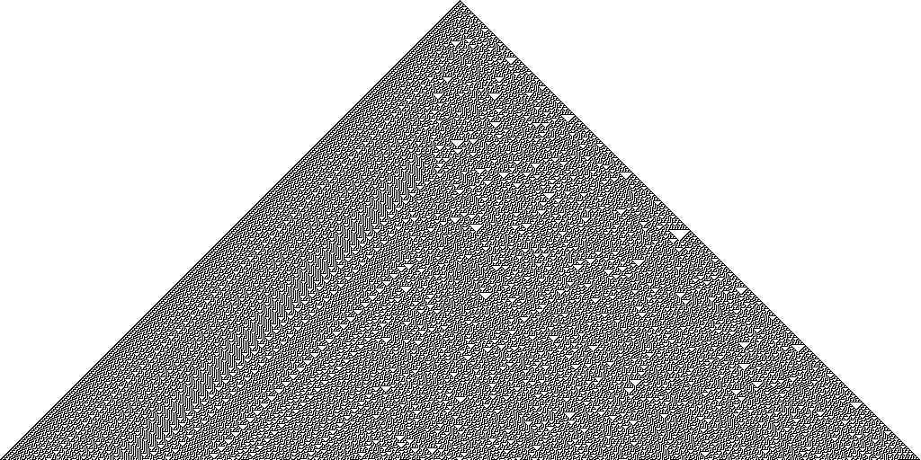

Rows vs Columns

In the last solution we generated the image column by column. Try to change the algorithm to write out row by row. The image will appear rotated. Did this affect the performance? Why do you think that is?

Show me the solution

JULIA

function run_eca_builder2(r::Int, n::Int)
    x = zeros(Bool, n)
    x[n÷2] = 1
    b = Vector{Bool}(undef, n)

    result = Array{Bool,2}(undef, n ÷ 2, n)
    result[1, :] .= x

    for i in 2:(n÷2)
        @views rule(r)(x, b)
        x, b = b, x
        result[i, :] .= x
    end
    return result
end

This should be significantly slower. Columns are consecutive in memory, making copying operations much easier for the CPU.

StaticArrays

We’ve actually already seen static arrays in use, when we used the Vec3d type to store three dimensional vectors in our gravity simulation. Static arrays can be very useful to reduce allocations of small arrays. In our case, the nb array can be made into a static array.

Beware, that the array size should be a static (compile time) argument now. It may be instructive to see what happens when you keep the sz argument as a tuple. Run the profile viewer to see that you have a type instability. Taking the argument as ::Size{sz} gets rid of this type instability. The stencil! function should now run nearly twice as fast.

Rerun the timings in the previous exercise to show that this is the case.

JULIA

#| id: stencils
"""
    stencil!(f, <: BoundaryType{dim}, Size{sz}, inp, out)

The function `f` should take an `AbstractArray` with size `sz` as input
and return a single value. Then, `stencil` applies the function `f` to a
neighbourhood around each element and writes the output to `out`. 
"""
function stencil!(f, ::Type{BT}, ::Size{sz}, inp::AbstractArray{T,dim}, out::AbstractArray{RT,dim}) where {dim, sz, BT <: BoundaryType{dim}, T, RT}
    @assert size(inp) == size(out)
    center = CartesianIndex((div.(sz, 2) .+ 1)...)
    for i in eachindex(IndexCartesian(), inp)
        nb = SArray{Tuple{sz...}, T}(
            get_bounded(BT, inp, i - center + j)
            for j in CartesianIndices(sz))
        out[i] = f(nb)
    end
    return out
end

stencil!(f, ::Type{BT}, sz) where {BT} =
    (inp, out) -> stencil!(f, BT, sz, inp, out)

JULIA

rule(n) = stencil!(eca(n), Periodic{1}, Size(3))

Game of Life

---

Game of Life is a two-dimensional cellular automaton, and probably the most famous one. We set the following rules:

• if there are three live neighbours, the cell lives.
• if there are less than two or more than three live neighbours, the cell dies.

JULIA

#| id: ca
game_of_life(a) = let s = sum(a) - a[2, 2]
    s == 3 || (a[2, 2] && s == 2)
end

a = rand(Bool, 64, 64)
b = zeros(Bool, 64, 64)
stencil!(game_of_life, Periodic{2}, Size(3, 3), a, b) |> to_image
a, b = b, a

Animated Life

Look up the documentation on animations in Makie. Can you make an animation of the Game of Life? Use the image! function with argument interpolation=false to show the image.

Show me the solution

Here’s a cool solution with live animation and lots more, just for your enjoyment.

JULIA

function tic(f, dt, running_)
    running::Observable{Bool} = running_

    @async begin
        while running[]
            sleep(dt[])
            f()
        end
    end
end

function run_life()
    fig = Figure()

    sz = (256, 256)
    state = Observable(rand(Bool, sz...))
    temp = Array{Bool, 2}(undef, sz...)
    foo = stencil!(game_of_life, Periodic{2}, Size(3, 3))

    function next()
        foo(state[], temp)
        state[], temp = temp, state[] # copy(temp)
    end

    ax = Makie.Axis(fig[1, 1], aspect=1)
    gb = GridLayout(fig[2, 1], tellwidth=false)

    playing = Observable(false)

    play_button_text = lift(p->(p ? "Pause" : "Play"), playing)
    play_button = gb[1,1] = Button(fig, label=play_button_text)
    rand_button = gb[1,2] = Button(fig, label="Randomize")
    speed_slider = gb[1,3] = SliderGrid(fig, (label="delay", range = logrange(0.001, 1.0, 100), startvalue=0.1))

    on(play_button.clicks) do _
        p = !playing[]
        playing[] = p
        if p
            tic(next, speed_slider.sliders[1].value, playing)
        end
    end

    on(rand_button.clicks) do _
        state[] = rand(Bool, sz...)
    end

    image!(ax, lift(to_image, state), interpolate=false)

    fig
end

run_life()

There are some nice libraries that you may want to look into:

• Stencils.jl for another implementation of stencils.
• Agents.jl for agent based modelling.

---

Key Points

• Value types are a useful and efficient abstraction
• Using StaticArrays can have a dramatic impact on performance

Source code

JULIA

#| file: src/Stencils.jl
module Stencils
    using StaticArrays

    <<stencils>>
end