Introduction to Working with MRI Data in Python: All in One View

Content from Before we start

Last updated on 2024-02-18 | Edit this page

Overview

Questions

What is Python and why should I learn it?

Objectives

Present motivations for using Python.
Organize files and directories for a set of analyses as a Python project.
How to work with Jupyter Notebook.
Know where to find help.

This overview have been adapted from the Data Carpentry Python Lessons with Ecological Data.

Why Python?

Python is rapidly becoming the standard language for data analysis, visualization and automated workflow building. It is a free and open-source software that is relatively easy to pick up by new programmers and is available on multiple operating systems. In addition, with Python packages such as Jupyter one can keep an interactive code journal of analysis - this is what we’ll be using in the workshop. Using Jupyter notebooks allows you to keep a record of all the steps in your analysis, enabling reproducibility and ease of code sharing.

Another advantage of Python is that it is maintained by a large user-base. Anyone can easily make their own Python packages for others to use. Therefore, there exists a very large codebase for you to take advantage of for your neuroimaging analysis; from basic statistical analysis, to brain visualization tools, to advanced machine learning and multivariate methods!

Knowing your way around Anaconda and Jupyter

The Anaconda distribution of Python includes a lot of its popular packages, such as the IPython console, and Jupyter Notebook. Have a quick look around the Anaconda Navigator. You can launch programs from the Navigator or use the command line.

The Jupyter notebook is an open-source web application that allows you to create and share documents that allow one to create documents that combine code, graphs, and narrative text. If you have not worked with Jupyter notebooks before, you might start with the tutorial from Jupyter.org called “Try Classic Notebook”.

Anaconda also comes with a package manager called conda, which makes it easy to install and update additional packages.

Organizing your working directory

Using a consistent folder structure across your projects will help you keep things organized, and will also make it easy to find/file things in the future. This can be especially helpful when you have multiple projects. In general, you may wish to create separate directories for your scripts, data, and documents.

This lesson uses the following folders to keep things organized:

data/: Use this folder to store your raw data. For the sake of transparency and provenance, you should always keep a copy of your raw data. If you need to cleanup data, do it programmatically (i.e. with scripts) and make sure to separate cleaned up data from the raw data. For example, you can store raw data in files ./data/raw/ and clean data in ./data/clean/.
code/: Use this folder to store your (Python) scripts for data cleaning, analysis, and plotting that you use in this particular project. This folder contains all of the Jupyter notebooks used in the lesson.
files/: Use this folder to store any miscellaneous outlines, drafts, and other text. This folder contains a set of Powerpoint slides that will be used for parts of the lesson.

How to learn more after the workshop?

The material we cover during this workshop will give you an initial taste of how you can use Python to analyze MRI data for your own research. However, you will need to learn more to do advanced operations such as working with specific MRI modalities, cleaning your dataset, using statistical methods, or creating beautiful graphics. The best way to become proficient and efficient at Python, as with any other tool, is to use it to address your actual research questions. As a beginner, it can feel daunting to have to write a script from scratch, and given that many people make their code available online, modifying existing code to suit your purpose might make it easier for you to get started.

Seeking help

check under the Help menu
type help()
type ?object or help(object) to get information about an object
Python documentation
NiBabel documentation

Finally, a generic Google or internet search “Python task” will often either send you to the appropriate module documentation or a helpful forum where someone else has already asked your question.

I am stuck… I get an error message that I don’t understand. Start by googling the error message. However, this doesn’t always work very well, because often, package developers rely on the error catching provided by Python. You end up with general error messages that might not be very helpful to diagnose a problem (e.g. “subscript out of bounds”). If the message is very generic, you might also include the name of the function or package you’re using in your query.

You can also check Stack Overflow. Most questions have already been answered, but the challenge is to use the right words in the search to find the answers.

Another helpful resource specific to the neuroimaging community is NeuroStars.

Key Points

Python is an open source and platform independent programming language.
Jupyter Notebook is a great tool to code in and interact with Python.
With the large Python community it is easy to find help on the internet.

Content from From the scanner to our computer

Last updated on 2024-02-28 | Edit this page

Overview

Questions

What are the main MRI modalities?
What’s the first step necessary to start working with MRI data?

Objectives

Understand how different MRI modalities differ and what each one represents
Become familiar with converting MRI data from DICOM to NIfTI

Types of MR scans

Anatomical

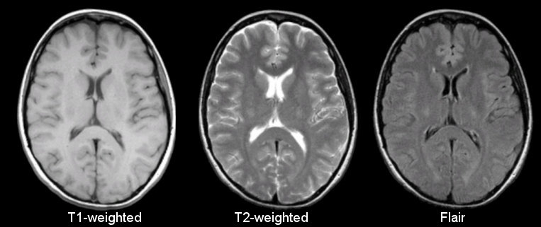
Sourced from https://case.edu/med/neurology/NR/MRI%20Basics.htm

3D image of anatomy (i.e., shape, volume, cortical thickness, brain region)
can differentiate tissue types

Functional

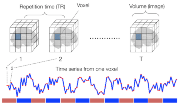
Sourced from Wagner and Lindquist, 2015

tracks the blood oxygen level-dependant (BOLD) signal as an analogue of brain activity
4D image (x, y, z + time)

Diffusion

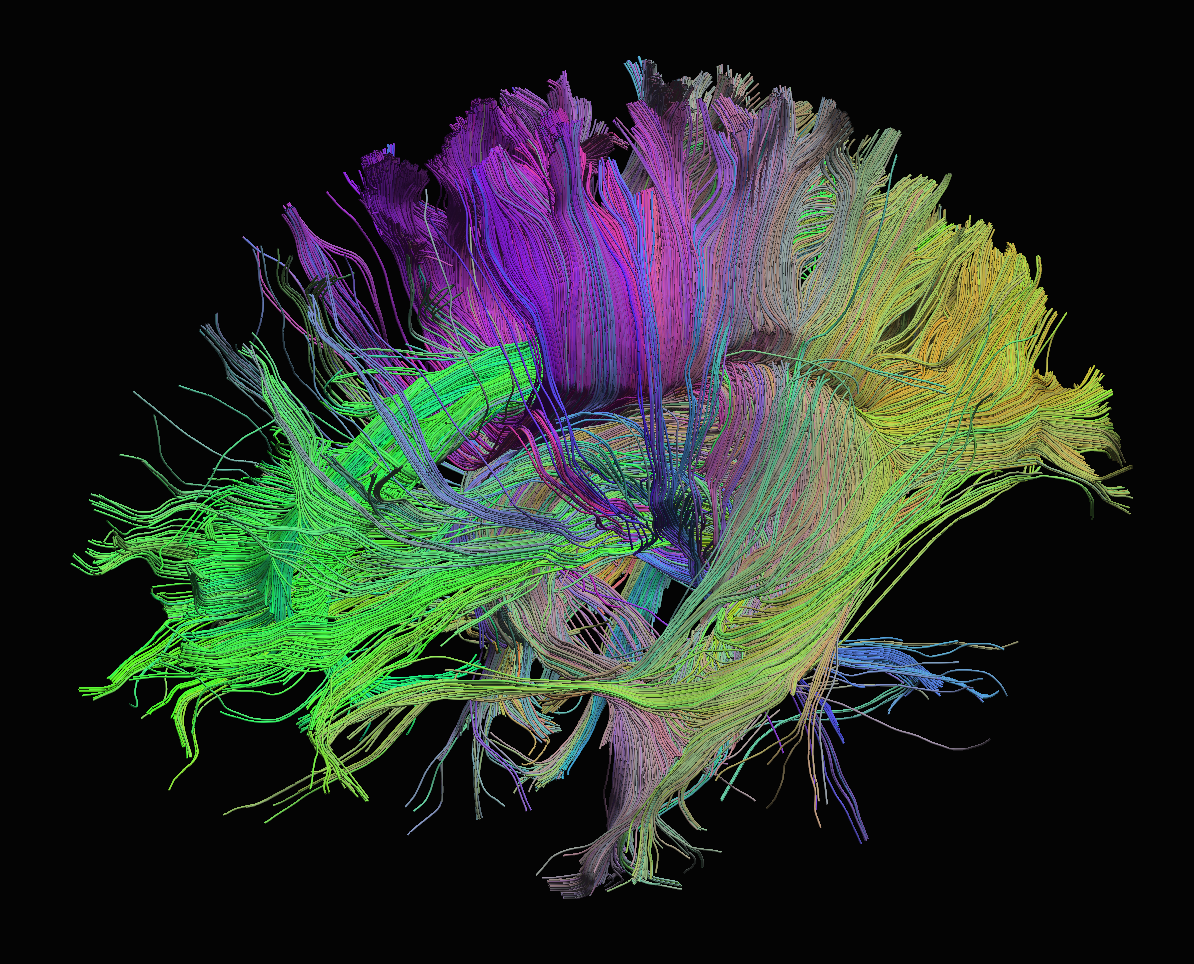
Sourced from http://brainsuite.org/processing/diffusion/tractography/

measures diffusion of water in order to model tissue microstructure
4D image (x, y, z + direction of diffusion)
need parameters about the strength of the diffusion “gradient” and its direction (.bval and .bvec)

Neuroimaging file formats

Format Name	File Extension	Origin
DICOM	none	ACR/NEMA Consortium
Analyze	.img/.hdr	Analyze Software, Mayo Clinic
NIfTI	.nii	Neuroimaging Informatics Technology Initiative
MINC	.mnc	Montreal Neurological Institute
NRRD	.nrrd

From the MRI scanner, images are initially collected in the DICOM format and can be converted to these other formats to make working with the data easier.

Let’s download some example DICOM data to see what it looks like. This data was generously shared publicly by the Princeton Handbook for Reproducible Neuroimaging.

BASH

wget https://zenodo.org/record/3677090/files/0219191_mystudy-0219-1114.tar.gz -O ../data/0219191_mystudy-0219-1114.tar.gz
mkdir -p ../data/dicom_examples
tar -xvzf ../data/0219191_mystudy-0219-1114.tar.gz -C ../data/dicom_examples
gzip -d ../data/dicom_examples/0219191_mystudy-0219-1114/dcm/*dcm.gz
rm ../data/0219191_mystudy-0219-1114.tar.gz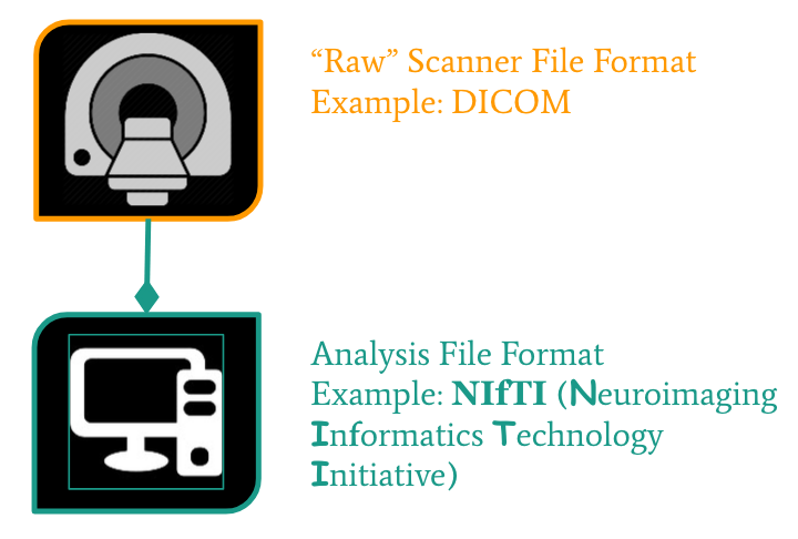

NIfTI is one of the most ubiquitous file formats for storing neuroimaging data. If you’re interested in learning more about NIfTI images, we highly recommend this blog post about the NIfTI format. We can convert our DICOM data to NIfTI using dcm2niix.

We can learn how to run dcm2niix by taking a look at its help menu.

BASH

dcm2niix -help

Converting DICOM to NIfTI

Convert the Princeton DICOM data to NIfTI

Show me the solution

BASH

mkdir -p ../data/dicom_examples/nii
dcm2niix -z y -o ../data/dicom_examples/nii ../data/dicom_examples/0219191_mystudy-0219-1114/

Key Points

MRI can capture anatomical (structural), functional, or diffusion features.
A number of file formats exist to store neuroimaging data.

Content from Anatomy of a NIfTI

Last updated on 2024-02-29 | Edit this page

Overview

Questions

How are MRI data represented digitally?

Objectives

Introduce Python data types
Load an MRI scan into Python and understand how the data is stored
Understand what a voxel is
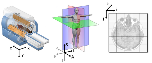
Introduce MRI coordinate systems
View and manipulate image data

In the last lesson, we introduced the NIfTI. We’ll cover a few details to get started working with them.

Reading NIfTI images

NiBabel is a Python package for reading and writing neuroimaging data. To learn more about how NiBabel handles NIfTIs, check out the Working with NIfTI images page of the NiBabel documentation, from which this episode is heavily based.

PYTHON

import nibabel as nib

First, use the load() function to create a NiBabel image object from a NIfTI file. We’ll load in an example T1w image from the zip file we just downloaded.

PYTHON

t1_img = nib.load("../data/dicom_examples/nii/0219191_mystudy-0219-1114_anat_ses-01_T1w_20190219111436_5.nii.gz")

Loading in a NIfTI file with NiBabel gives us a special type of data object which encodes all the information in the file.Each bit of information is called an attribute in Python’s terminology. To see all of these attributes, type t1_img. followed by Tab. There are three main attributes that we’ll discuss today:

1. Header: contains metadata about the image, such as image dimensions, data type, etc.

PYTHON

t1_hdr = t1_img.header
print(t1_hdr)

OUTPUT

<class 'nibabel.nifti1.Nifti1Header'> object, endian='<'
sizeof_hdr      : 348
data_type       : b''
db_name         : b''
extents         : 0
session_error   : 0
regular         : b''
dim_info        : 0
dim             : [ 3 57 67 56  1  1  1  1]
intent_p1       : 0.0
intent_p2       : 0.0
intent_p3       : 0.0
intent_code     : none
datatype        : uint8
bitpix          : 8
slice_start     : 0
pixdim          : [1.   2.75 2.75 2.75 1.   1.   1.   1.  ]
vox_offset      : 0.0
scl_slope       : nan
scl_inter       : nan
slice_end       : 0
slice_code      : unknown
xyzt_units      : 2
cal_max         : 0.0
cal_min         : 0.0
slice_duration  : 0.0
toffset         : 0.0
glmax           : 0
glmin           : 0
descrip         : b''
aux_file        : b''
qform_code      : mni
sform_code      : mni
quatern_b       : 0.0
quatern_c       : 0.0
quatern_d       : 0.0
qoffset_x       : -78.0
qoffset_y       : -91.0
qoffset_z       : -91.0
srow_x          : [  2.75   0.     0.   -78.  ]
srow_y          : [  0.     2.75   0.   -91.  ]
srow_z          : [  0.     0.     2.75 -91.  ]
intent_name     : b''
magic           : b'n+1'

t1_hdr is a Python dictionary. Dictionaries are containers that hold pairs of objects - keys and values. Let’s take a look at all of the keys. Similar to t1_img in which attributes can be accessed by typing t1_img. followed by Tab, you can do the same with t1_hdr. In particular, we’ll be using a method belonging to t1_hdr that will allow you to view the keys associated with it.

PYTHON

t1_hdr.keys()

OUTPUT

['sizeof_hdr',
 'data_type',
 'db_name',
 'extents',
 'session_error',
 'regular',
 'dim_info',
 'dim',
 'intent_p1',
 'intent_p2',
 'intent_p3',
 'intent_code',
 'datatype',
 'bitpix',
 'slice_start',
 'pixdim',
 'vox_offset',
 'scl_slope',
 'scl_inter',
 'slice_end',
 'slice_code',
 'xyzt_units',
 'cal_max',
 'cal_min',
 'slice_duration',
 'toffset',
 'glmax',
 'glmin',
 'descrip',
 'aux_file',
 'qform_code',
 'sform_code',
 'quatern_b',
 'quatern_c',
 'quatern_d',
 'qoffset_x',
 'qoffset_y',
 'qoffset_z',
 'srow_x',
 'srow_y',
 'srow_z',
 'intent_name',
 'magic']

Notice that methods require you to include () at the end of them whereas attributes do not. The key difference between a method and an attribute is:

Attributes are stored values kept within an object
Methods are processes that we can run using the object. Usually a method takes attributes, performs an operation on them, then returns it for you to use.

When you type in t1_img. followed by Tab, you’ll see that attributes are highlighted in orange and methods highlighted in blue.

The output above is a list of keys you can use from t1_hdr to access values. We can access the value stored by a given key by typing:

PYTHON

t1_hdr['<key_name>']

Extract values from the NIfTI header

Extract the value of pixdim from t1_hdr

Show me the solution

PYTHON

t1_hdr['pixdim']

OUTPUT

array([1.  , 2.75, 2.75, 2.75, 1.  , 1.  , 1.  , 1.  ], dtype=float32)

2. Data

As you’ve seen above, the header contains useful information that gives us information about the properties (metadata) associated with the MR data we’ve loaded in. Now we’ll move in to loading the actual image data itself. We can achieve this by using the method called t1_img.get_fdata().

PYTHON

t1_data = t1_img.get_fdata()
t1_data

OUTPUT

array([[[ 8.79311806,  8.79311806,  8.79311806, ...,  7.73574093,
          7.73574093,  7.38328189],
        [ 8.79311806,  9.1455771 ,  8.79311806, ...,  8.08819997,
          8.08819997,  8.08819997],
        [ 9.1455771 ,  8.79311806,  8.79311806, ...,  8.44065902,
          8.44065902,  8.44065902],
        ...,
        [ 8.08819997,  8.44065902,  8.08819997, ...,  7.38328189,
          7.38328189,  7.38328189],
        [ 8.08819997,  8.08819997,  8.08819997, ...,  7.73574093,
          7.38328189,  7.38328189],
        [ 8.08819997,  8.08819997,  8.08819997, ...,  7.38328189,
          7.38328189,  7.03082284]],

       [[ 8.79311806,  9.1455771 ,  8.79311806, ...,  7.73574093,
          7.38328189,  7.38328189],
        [ 8.79311806,  9.1455771 ,  9.1455771 , ...,  8.08819997,
          7.73574093,  8.08819997],
        [ 8.79311806,  9.49803615,  9.1455771 , ...,  8.44065902,
          8.44065902,  8.44065902],
        ...,
        [ 8.08819997,  8.08819997,  8.08819997, ...,  7.38328189,
          7.38328189,  7.03082284],
        [ 8.08819997,  8.08819997,  8.08819997, ...,  7.38328189,
          7.38328189,  7.38328189],
        [ 8.08819997,  8.08819997,  8.08819997, ...,  7.38328189,
          7.38328189,  7.73574093]],

       [[ 9.1455771 ,  9.1455771 ,  8.79311806, ...,  7.73574093,
          7.38328189,  7.03082284],
        [ 9.1455771 ,  9.49803615,  9.1455771 , ...,  8.08819997,
          7.73574093,  7.38328189],
        [ 9.1455771 ,  9.49803615,  9.1455771 , ...,  8.08819997,
          8.08819997,  8.08819997],
        ...,
        [ 8.08819997,  8.44065902,  8.44065902, ...,  7.73574093,
          7.38328189,  7.38328189],
        [ 8.44065902,  8.08819997,  8.44065902, ...,  7.38328189,
          7.38328189,  7.38328189],
        [ 8.08819997,  8.08819997,  8.08819997, ...,  7.38328189,
          7.38328189,  7.38328189]],

       ...,

       [[ 9.49803615,  9.85049519,  9.85049519, ...,  7.38328189,
          7.38328189,  7.03082284],
        [ 9.85049519,  9.85049519,  9.85049519, ...,  7.38328189,
          7.38328189,  7.73574093],
        [ 9.85049519,  9.85049519, 10.20295423, ...,  8.08819997,
          8.08819997,  8.08819997],
        ...,
        [ 9.49803615,  9.1455771 ,  9.49803615, ...,  7.73574093,
          7.73574093,  7.73574093],
        [ 9.49803615,  9.49803615,  9.1455771 , ...,  7.73574093,
          8.08819997,  7.73574093],
        [ 9.49803615,  9.1455771 ,  8.79311806, ...,  8.08819997,
          7.73574093,  7.73574093]],

       [[ 9.49803615,  9.85049519, 10.20295423, ...,  7.38328189,
          7.38328189,  7.03082284],
        [ 9.1455771 ,  9.85049519,  9.1455771 , ...,  7.73574093,
          7.38328189,  7.38328189],
        [ 9.85049519,  9.85049519,  9.49803615, ...,  8.08819997,
          7.73574093,  8.08819997],
        ...,
        [ 9.49803615,  8.79311806,  9.1455771 , ...,  8.08819997,
          7.38328189,  7.73574093],
        [ 9.1455771 ,  9.1455771 ,  9.1455771 , ...,  7.73574093,
          8.08819997,  7.73574093],
        [ 8.79311806,  9.1455771 ,  9.1455771 , ...,  7.73574093,
          7.73574093,  7.38328189]],

       [[ 9.1455771 ,  8.79311806,  8.79311806, ...,  7.03082284,
          7.03082284,  6.6783638 ],
        [ 9.49803615,  9.85049519,  9.49803615, ...,  7.73574093,
          7.73574093,  7.73574093],
        [ 9.49803615,  9.49803615,  9.85049519, ...,  7.73574093,
          8.08819997,  7.73574093],
        ...,
        [ 8.79311806,  9.1455771 ,  9.1455771 , ...,  8.08819997,
          8.08819997,  8.08819997],
        [ 9.1455771 ,  9.1455771 ,  9.1455771 , ...,  8.08819997,
          8.08819997,  7.73574093],
        [ 8.79311806,  9.1455771 ,  9.1455771 , ...,  8.08819997,
          7.73574093,  7.73574093]]])

What type of data is this exactly? We can determine this by calling the type() function on t1_data.

PYTHON

type(t1_data)

OUTPUT

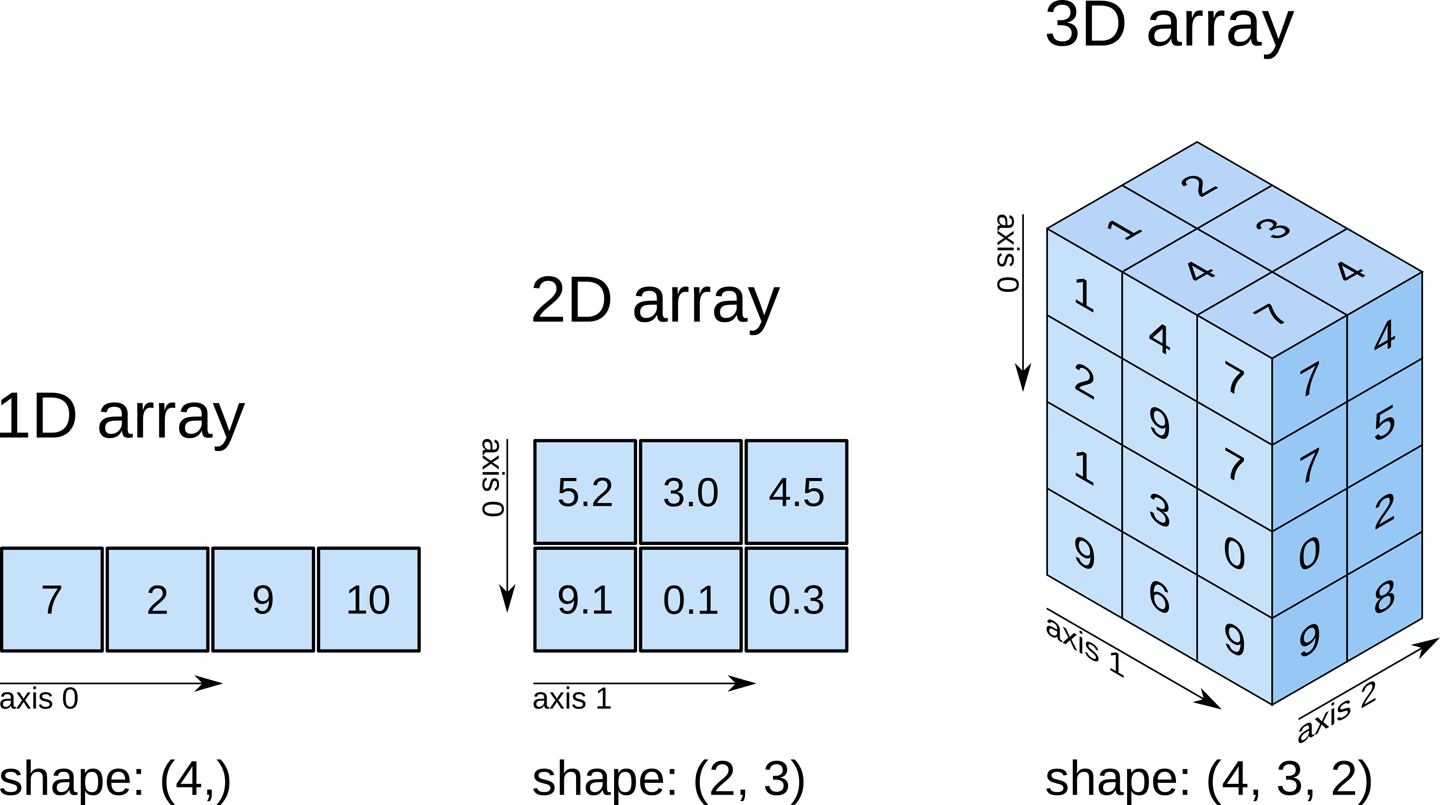
numpy.ndarray

The data is a multidimensional array representing the image data. In Python, an array is used to store lists of numerical data into something like a table.

Check out attributes of the array

How can we see the number of dimensions in the t1_data array? Once again, all of the attributes of the array can be seen by typing t1_data. followed by Tab.

Show me the solution

PYTHON

t1_data.ndim

OUTPUT

t1_data contains 3 dimensions. You can think of the data as a 3D version of a picture (more accurately, a volume).

Check out attributes of the array(continued)

While typical 2D pictures are made out of squares called pixels, a 3D MR image is made up of 3D cubes called voxels.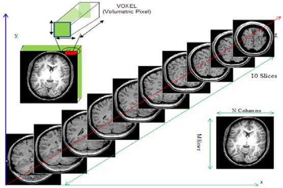
What about the how big each dimension is (shape)?

Show me the solution

PYTHON

t1_data.shape

OUTPUT

(57, 67, 56)

The 3 numbers given here represent the number of values along a respective dimension (x,y,z). This brain was scanned in 57 slices with a resolution of 67 x 56 voxels per slice. That means there are:

57 * 67 * 56 = 213864

voxels in total!

Let’s see the type of data inside of the array.

PYTHON

t1_data.dtype

OUTPUT

dtype('float64')

This tells us that each element in the array (or voxel) is a floating-point number.
The data type of an image controls the range of possible intensities. As the number of possible values increases, the amount of space the image takes up in memory also increases.

PYTHON

import numpy as np
print(np.min(t1_data))
print(np.max(t1_data))

OUTPUT

6.678363800048828
96.55541983246803

For our data, the range of intensity values goes from 0 (black) to more positive digits (whiter).

How do we examine what value a particular voxel is? We can inspect the value of a voxel by selecting an index as follows:

data[x,y,z]

So for example we can inspect a voxel at coordinates (10,20,3) by doing the following:

PYTHON

t1_data[9, 19, 2]

OUTPUT

32.40787395834923

NOTE: Python uses zero-based indexing. The first item in the array is item 0. The second item is item 1, the third is item 2, etc.

This yields a single value representing the intensity of the signal at a particular voxel! Next we’ll see how to not just pull one voxel but a slice or an array of voxels for visualization and analysis!

Working with image data

Slicing does exactly what it seems to imply. Giving our 3D volume, we pull out a 2D slice of our data.

From left to right: sagittal, coronal and axial slices.

Let’s pull the 10th slice in the x axis.

PYTHON

x_slice = t1_data[9, :, :]

This is similar to the indexing we did before to pull out a single voxel. However, instead of providing a value for each axis, the : indicates that we want to grab all values from that particular axis.

Slicing MRI data

Now try selecting the 20th slice from the y axis.

Show me the solution

PYTHON

y_slice = t1_data[:, 19, :]

Slicing MRI data(continued)

Finally, try grabbing the 3rd slice from the z axis

Show me the solution

PYTHON

z_slice = t1_data[:, :, 2]

We’ve been slicing and dicing brain images but we have no idea what they look like! In the next section we’ll show you how you can visualize brain slices!

Visualizing the data

We previously inspected the signal intensity of the voxel at coordinates (10,20,3). Let’s see what out data looks like when we slice it at this location. We’ve already indexed the data at each x, y, and z axis. Let’s use matplotlib.

PYTHON

import matplotlib.pyplot as plt
%matplotlib inline

slices = [x_slice, y_slice, z_slice]

fig, axes = plt.subplots(1, len(slices))
for i, slice in enumerate(slices):
    axes[i].imshow(slice.T, cmap="gray", origin="lower")

Now, we’re going to step away from discussing our data and talk about the final important attribute of a NIfTI.

3. Affine: tells the position of the image array data in a reference space

The final important piece of metadata associated with an image file is the affine matrix. Below is the affine matrix for our data.

PYTHON

t1_affine = t1_img.affine
t1_affine

OUTPUT

array([[  2.75,   0.  ,   0.  , -78.  ],
       [  0.  ,   2.75,   0.  , -91.  ],
       [  0.  ,   0.  ,   2.75, -91.  ],
       [  0.  ,   0.  ,   0.  ,   1.  ]])

To explain this concept, recall that we referred to coordinates in our data as (x,y,z) coordinates such that:

x is the first dimension of t1_data
y is the second dimension of t1_data
z is the third dimension of t1_data

Although this tells us how to access our data in terms of voxels in a 3D volume, it doesn’t tell us much about the actual dimensions in our data (centimetres, right or left, up or down, back or front). The affine matrix allows us to translate between voxel coordinates in (x,y,z) and world space coordinates in (left/right,bottom/top,back/front). An important thing to note is that in reality in which order you have:

left/right
bottom/top
back/front

Depends on how you’ve constructed the affine matrix, but for the data we’re dealing with it always refers to:

Right
Anterior
Superior

Applying the affine matrix (t1_affine) is done through using a linear map (matrix multiplication) on voxel coordinates (defined in t1_data).

The concept of an affine matrix may seem confusing at first but an example might help gain an intuition:

Suppose we have two voxels located at the the following coordinates: \((64, 100, 2)\)

And we wanted to know what the distances between these two voxels are in terms of real world distances (millimetres). This information cannot be derived from using voxel coordinates so we turn to the affine matrix.

Now, the affine matrix we’ll be using happens to be encoded in RAS. That means once we apply the matrix our coordinates are as follows:
(Right, Anterior, Superior)

So increasing a coordinate value in the first dimension corresponds to moving to the right of the person being scanned.

Applying our affine matrix yields the following coordinates: \((10.25, 30.5, 9.2)\)

This means that:

Voxel 1 is 90.23 - 10.25 = 79.98 in the R axis. Positive values mean move right
Voxel 1 is 0.2 - 30.5 = -30.3 in the A axis. Negative values mean move posterior
Voxel 1 is 2.15 - 9.2 = -7.05 in the S axis. Negative values mean move inferior

This covers the basics of how NIfTI data and metadata are stored and organized in the context of Python. In the next segment we’ll talk a bit about an increasingly important component of MR data analysis - data organization. This is a key component to reproducible analysis and so we’ll spend a bit of time here.

Key Points

NIfTI image contain a header, which describes the contents, and the data.
The position of the NIfTI data in space is determined by the affine matrix.
NIfTI data is a multi-dimensional array of values.

Content from Data organization with BIDS

Last updated on 2024-02-28 | Edit this page

Overview

Questions

What is BIDS?
Why is it important to structure our datasets coherently?
How can we convert raw datasets into BIDS-compatible datasets?

Objectives

Become faimiliar with BIDS
Convert raw datasets to BIDS-compatible datasets

Brain Imaging Data Structure (BIDS) is a simple and intuitive way to organize and describe your neuroimaging and behavioural data. Neuroimaging experiments result in complicated data that can be arranged in several different ways. BIDS tackles this problem by suggesting a new standard (based on consensus from multiple researchers across the world) for the arrangement of neuroimaging datasets.

Using the same structure for all of your studies will allow you to easily reuse all of your scripts between studies. Additionally, sharing code with other researchers will be much easier.

Why convert the community to BIDS?

A common file structure for both computers and humans to understand
Using file formats/conventions that are most common in neuroimaging
Show completeness of the data right away

Build better pipelines:

All the information you need to design a pipeline for a particular dataset is machine readable
Pipelines can be more complex (under the hood) with fewer command-line arguments

bidsifying your dataset:

Convert your (raw) MRI data to the BIDS-compatible dataset format

Key Points

BIDS is an organizational principle for neuroimaging data.
Converting a raw MRI dataset to a BIDS-compatible dataset streamlines data processing pipelines.

Content from Exploring open MRI datasets

Last updated on 2024-02-28 | Edit this page

Overview

Questions

How does standardizing neuroimaging data ease the data exploration process

Objectives

Understand the BIDS format
Use PyBIDS in to easily explore a BIDS dataset

Tutorial Dataset

In this episode, we will be using a subset of a publicly available dataset, ds000030, from openneuro.org. All of the datasets on OpenNeuro are already structured according to BIDS.

Downloading Data

DataLad

DataLad installs the data - which for a dataset means that we get the “small” data (i.e. the text files) and the download instructions for the larger files. We can now navigate the dataset like its a part of our file system and plan our analysis.

First, navigate to the folder where you’d like to download the dataset.

BASH

cd ~/Desktop/dc-mri/data
datalad install ///openneuro/ds000030

Let’s take a look at the participants.tsv file to see what the demographics for this dataset look like.

PYTHON

import pandas as pd

participant_metadata = pd.read_csv('../data/ds000030/participants.tsv', sep='\t')
participant_metadata

OUTPUT:

	participant_id	diagnosis	age	gender	bart	bht	dwi	pamenc	pamret	rest	scap	stopsignal	T1w	taskswitch	ScannerSerialNumber	ghost_NoGhost
0	sub-10159	CONTROL	30	F	1.0	NaN	1.0	NaN	NaN	1.0	1.0	1.0	1.0	1.0	35343.0	No_ghost
1	sub-10171	CONTROL	24	M	1.0	1.0	1.0	NaN	NaN	1.0	1.0	1.0	1.0	1.0	35343.0	No_ghost
2	sub-10189	CONTROL	49	M	1.0	NaN	1.0	NaN	NaN	1.0	1.0	1.0	1.0	1.0	35343.0	No_ghost
3	sub-10193	CONTROL	40	M	1.0	NaN	1.0	NaN	NaN	NaN	NaN	NaN	1.0	NaN	35343.0	No_ghost
4	sub-10206	CONTROL	21	M	1.0	NaN	1.0	NaN	NaN	1.0	1.0	1.0	1.0	1.0	35343.0	No_ghost

From this table we can easily view unique diagnostic groups:

PYTHON

participant_metadata['diagnosis'].unique()

OUTPUT

array(['CONTROL', 'SCHZ', 'BIPOLAR', 'ADHD'], dtype=object)

Imagine we’d like to work with participants that are either CONTROL or SCHZ (diagnosis) and have both a T1w (T1w == 1) and rest (rest == 1) scan. Also, you’ll notice some of the T1w scans included in this dataset have a ghosting artifact. We’ll need to filter these out as well (ghost_NoGhost == 'No_ghost').

We’ll filter this data out like so:

PYTHON

participant_metadata = participant_metadata[(participant_metadata.diagnosis.isin(['CONTROL', 'SCHZ'])) &
                                            (participant_metadata.T1w == 1) &
                                            (participant_metadata.rest == 1) &
                                            (participant_metadata.ghost_NoGhost == 'No_ghost')]
participant_metadata['diagnosis'].unique()

OUTPUT

array(['CONTROL', 'SCHZ'], dtype=object)

From this we have a list of participants corresponding to a list of participants who are of interest in our analysis. We can then use this list in order to download participant from software such as aws or datalad. In fact, this is exactly how we set up a list of participants to download for the fMRI workshop! Since we’ve already downloaded the dataset, we can now explore the structure using PyBIDS, a Python API for querying, summarizing and manipulating the BIDS folder structure.

Getting and dropping data

datalad get datalad drop

PYTHON

from bids.layout import BIDSLayout

layout = BIDSLayout("~/Desktop/dc-mri/data/ds000030")

The pybids layout object indexes the BIDS folder. Indexing can take a really long time, especially if you have several subjects, modalities, scan types, etc. pybids has an option to save the indexed results to a SQLite database. This database can then be re-used the next time you want to query the same BIDS folder.

PYTHON

layout.save("~/Desktop/dc-mri/data/ds000030/.db")

layout = BIDSLayout("~/Desktop/dc-mri/data/ds000030", database_path="~/Desktop/dc-mri/data/ds000030/.db")

The pybids layout object also lets you query your BIDS dataset according to a number of parameters by using a get_*() method. We can get a list of the subjects we’ve downloaded from the dataset.

PYTHON

layout.get_subjects()

OUTPUT

['10171',
 '10292',
 '10365',
 '10438',
 '10565',
 '10788',
 '11106',
 '11108',
 '11122',
   ...
 '50083']

We can also pull a list of imaging modalities in the dataset:

PYTHON

layout.get_modalities()

OUTPUT

['anat', 'func']

As well as tasks and more!:

PYTHON

#Task fMRI
print(layout.get_tasks())

#Data types (bold, brainmask, confounds, smoothwm, probtissue, warp...)
print(layout.get_types())

OUTPUT

['rest']

['bold',
 'brainmask',
 'confounds',
 'description',
 'dtissue',
 'fsaverage5',
 'inflated',
 'midthickness',
 'participants',
 'pial',
 'preproc',
 'probtissue',
 'smoothwm',
 'warp']

In addition we can specify sub-types of each BIDS category:

PYTHON

layout.get_types(modality='func')

OUTPUT

['brainmask', 'confounds', 'fsaverage5', 'preproc']

We can use this functionality to pull all our fMRI NIfTI files:

PYTHON

layout.get(task='rest', type='bold', extensions='nii.gz', return_type='file')

OUTPUT

TO FILL

Finally, we can convert the data stored in bids.layout into a pandas.DataFrame :

PYTHON

df = layout.as_data_frame()
df.head()

OUTPUT:

	path	modality	subject	task	type
0	~/Desktop/dc-mri/data…	NaN	NaN	rest	bold
1	~/Desktop/dc-mri/data…	NaN	NaN	NaN	participants
2	~/Desktop/dc-mri/data…	NaN	NaN	NaN	NaN
3	~/Desktop/dc-mri/data…	anat	10565	NaN	brainmask
4	~/Desktop/dc-mri/data…	anat	10565	NaN	probtissue

Key Points

Public neuroimaging BIDS-compatible data repositories allow for pulling data easily.
PyBIDS is a Python-based tool that allows for easy exploration of BIDS-formatted neuroimaging data.

Content from BIDS derivatives

Last updated on 2024-02-28 | Edit this page

Overview

Questions

What are BIDS Apps?
What are containers?

Objectives

Learn about neuroimaging applications using BIDS data structures
Use neuroimaging applications through containers

BIDS Apps are containerized applications that run on BIDS data structures.

Some examples include:

mriqc
fmriprep
freesurfer
ciftify
SPM
MRtrix3_connectome

They rely on 2 technologies for container computing:

Docker
- for building, hosting, and running containers on local hardware (Windows, Mac OS, Linux) or in the cloud
Singularity
- for running containers on high performance compute clusters

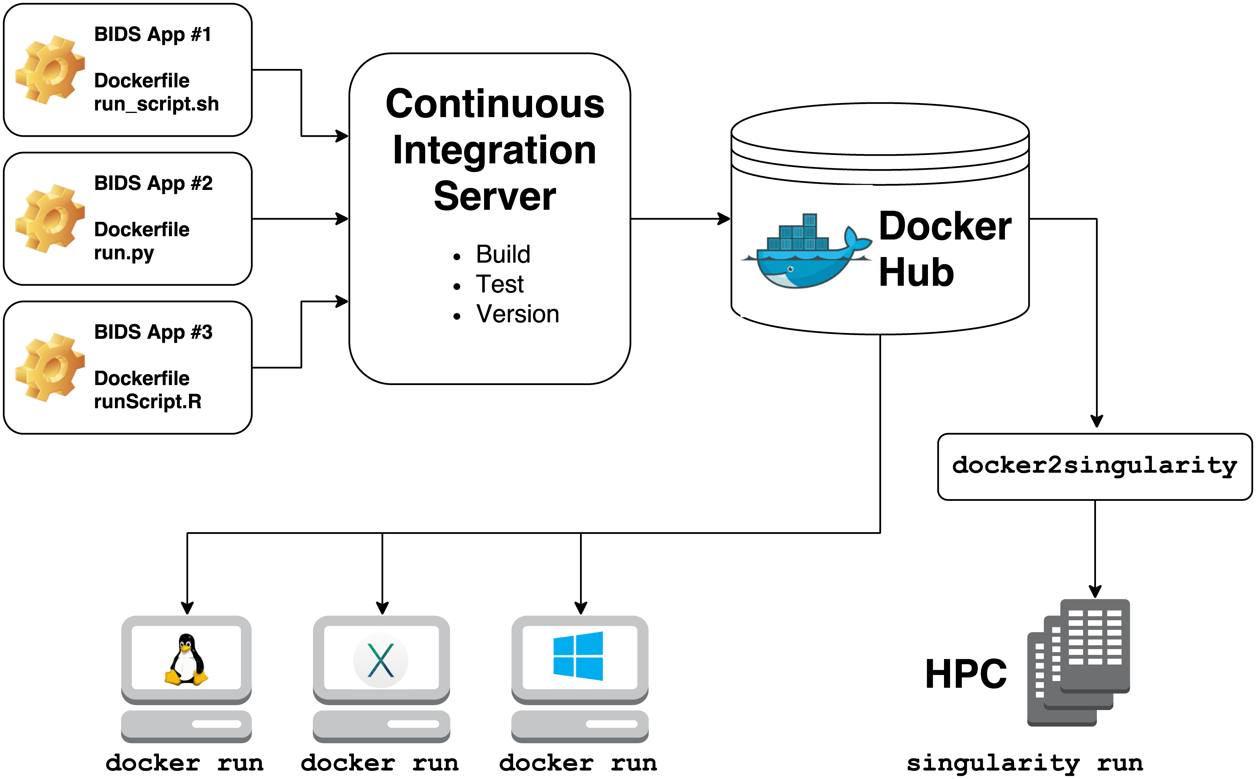
Building a singularity container is as easy as:

BASH

singularity build mriqc-0.16.1.simg docker://poldracklab/mriqc:0.16.1`

To run the container:

BASH

singularity run --cleanenv \
  -B bids_folder:/data \
  mriqc-0.16.1.simg \
  /data /data/derivatives participant

Key Points

BIDS Apps are containerized applications that run on BIDS-compatible datasets.

Overview

Questions

Objectives

Why Python?

Knowing your way around Anaconda and Jupyter

Organizing your working directory

How to learn more after the workshop?

Seeking help

Key Points

Overview

Questions

Objectives

Types of MR scans

Anatomical

Functional

Diffusion

Neuroimaging file formats

BASH

BASH

Converting DICOM to NIfTI

Show me the solution

BASH

Key Points

Overview

Questions

Objectives

Reading NIfTI images

PYTHON

PYTHON

1. Header: contains metadata about the image, such as image dimensions, data type, etc.

PYTHON

OUTPUT

PYTHON

OUTPUT

PYTHON

Extract values from the NIfTI header

Show me the solution

PYTHON

OUTPUT

2. Data

PYTHON

OUTPUT

PYTHON

OUTPUT

Check out attributes of the array

Show me the solution

PYTHON

OUTPUT

Check out attributes of the array(continued)

Show me the solution

PYTHON

OUTPUT

PYTHON

OUTPUT

PYTHON

OUTPUT

PYTHON

OUTPUT

Working with image data

PYTHON

Slicing MRI data

Show me the solution

PYTHON

Slicing MRI data(continued)

Show me the solution

PYTHON

Visualizing the data

PYTHON

3. Affine: tells the position of the image array data in a reference space

PYTHON

OUTPUT

Key Points

Overview

Questions

Objectives

Why convert the community to BIDS?

Share data:

Build better pipelines:

bidsifying your dataset:

Key Points