Minimal Reproducible Code

Last updated on 2025-05-09 | Edit this page

Estimated time: 75 minutes

Overview

Questions

Why is it important to make a minimal code example?
Which part of my code is causing the problem?
Which parts of my code should I include in a minimal example?
How can I tell whether a code snippet is reproducible or not?
How can I make my code reproducible?

Objectives

XXX updateme
Explain the value of a minimal code snippet.
Identify the problem area of a script.
Identify supporting parts of the code that are essential to include.
Simplify a script down to a minimal code example.
Evaluate whether a piece of code is reproducible as is or not. If not, identify what is missing.
Edit a piece of code to make it reproducible
Have a road map to follow to simplify your code.
Describe the {reprex} package and its uses

OUTPUT


Attaching package: 'dplyr'

OUTPUT

The following objects are masked from 'package:stats':

    filter, lag

OUTPUT

The following objects are masked from 'package:base':

    intersect, setdiff, setequal, union

Mickey is interested in understanding how kangaroo rat weights differ across species and sexes, so they create a quick visualization.

R

ggplot(rodents, aes(x = species, fill = sex))+
  geom_bar()

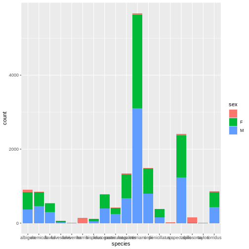Whoa, this is really overwhelming! Mickey forgot that the dataset includes data for a lot of different rodent species, not just kangaroo rats. Mickey is only interested in two kangaroo rat species: Dipodomys ordii (Ord’s kangaroo rat) and Dipodomys spectabilis (Banner-tailed kangaroo rat).

Mickey also notices that there are three categories for sex: F, M, and what looks like a blank field when there is no sex information available. For the purposes of comparing weights, Mickey wants to focus only rodents of known sex.

Mickey filters the data to include only the two focal species and only rodents whose sex is F or M.

R

rodents_subset <- rodents %>%
  filter(species == c("ordii", "spectabilis"),
         sex == c("F", "M"))

Because these scientific names are long, Mickey also decides to add common names to the dataset. They start by creating a data frame with the common names, which they will then join to the rodents_subset dataset:

R

## Adding common names
common_names <- data.frame(species = unique(rodents_subset$species), common_name = c("Ord's", "Banner-tailed"))
common_names

OUTPUT

      species   common_name
1 spectabilis         Ord's
2       ordii Banner-tailed

But looking at the common names dataset reveals a problem!

Applying code first aid

Is this a syntax error or a semantic error? Explain why.
What “code first aid” steps might be appropriate here? Which ones are unlikely to be helpful?

Mickey re-orders the names and tries the code again. This time, it works! Now they can join the common names to rodents_subset.

R

common_names <- data.frame(species = sort(unique(rodents_subset$species)), common_name = c("Ord's", "Banner-Tailed"))
common_names

OUTPUT

      species   common_name
1       ordii         Ord's
2 spectabilis Banner-Tailed

R

rodents_subset <- left_join(rodents_subset, common_names)

OUTPUT

Joining with `by = join_by(species)`

Before moving on to answering their research question about kangaroo rat weights, Mickey also wants to create a date column, since they realized that having the dates stored in three separate columns (month, day, and year) might be hard for future analysis. They want to use lubridate to parse the dates. But here, too, they run into trouble.

R

rodents_subset <- rodents_subset %>%
  mutate(date = lubridate(paste(year, month, day, sep = "-")))

ERROR

Error in `mutate()`:
ℹ In argument: `date = lubridate(paste(year, month, day, sep = "-"))`.
Caused by error in `lubridate()`:
! could not find function "lubridate"

:::instructor note Because these are fairly simple errors, more advanced learners may quickly “see” the solution and may need to be reminded to think through the exercise step by step and consider what steps could be helpful. Optionally, they can also be assigned the extra challenge exercise. :::

Applying code first aid, part 2

Is this a syntax error or a semantic error? Explain why.
What “code first aid” steps might be appropriate here?
What would be your next step to fix this error, if you were Mickey?

Applying code first aid, part 2 (extra challenge)

Mickey tried several methods to create a date column. Here’s one of them.

R

test <- rodents_subset %>%
  mutate(date = lubridate::as_date(paste(day, month, year)))

WARNING

Warning: There was 1 warning in `mutate()`.
ℹ In argument: `date = lubridate::as_date(paste(day, month, year))`.
Caused by warning:
! All formats failed to parse. No formats found.

What type of error is this?
What do you learn from the warning message? Why do you think this code causes a warning message, rather than an error message?
Try some code first aid steps. What do you think happened here? How did you figure it out?

Mickey reads some of the lubridate documentation and changes their code so that the date column is created correctly.

R

rodents_subset <- rodents_subset %>%
  mutate(date = lubridate::ymd(paste(year, month, day, sep = "-")))

Now that the dataset is cleaned, Mickey is ready to start learning about kangaroo rat weights!

They start by running a quick linear regression to predict weight based on species and sex.

R

weight_model <- lm(weight ~ common_name + sex, data = rodents_subset)
summary(weight_model)

OUTPUT


Call:
lm(formula = weight ~ common_name + sex, data = rodents_subset)

Residuals:
     Min       1Q   Median       3Q      Max
-111.201   -6.466    2.534   10.799   45.799

Coefficients: (1 not defined because of singularities)
                 Estimate Std. Error t value Pr(>|t|)
(Intercept)      123.2007     0.8061  152.83   <2e-16 ***
common_nameOrd's -74.7342     1.3352  -55.97   <2e-16 ***
sexM                   NA         NA      NA       NA
---
Signif. codes:  0 '***' 0.001 '**' 0.01 '*' 0.05 '.' 0.1 ' ' 1

Residual standard error: 19.71 on 939 degrees of freedom
  (35 observations deleted due to missingness)
Multiple R-squared:  0.7694,	Adjusted R-squared:  0.7691
F-statistic:  3133 on 1 and 939 DF,  p-value: < 2.2e-16

The negative coefficient for common_nameOrd's tells Mickey that Ord’s kangaroo rats are significantly less heavy than Banner-tailed kangaroo rats.

But something looks wrong with the coefficients for sex! Why is everything NA for sexM?

Mickey realizes that before creating a model, they should have re-visualized the dataset to make sure everything looked correct. They make a boxplot of kangaroo rat weights by species and sex, putting the species common names on the x axis and coloring by sex. They expect to see one box for each species-sex combination.

R

rodents_subset %>%
  ggplot(aes(y = weight, x = common_name, fill = sex)) +
  geom_boxplot()

WARNING

Warning: Removed 35 rows containing non-finite outside the scale range
(`stat_boxplot()`).

As the model showed, Ord’s kangaroo rats are significantly smaller than Banner-tailed kangaroo rats. But something is definitely wrong! Because the boxes are colored by sex, we can see that all of the Banner-tailed kangaroo rats are male and all of the Ord’s kangaroo rats are female. That can’t be right! What are the chances of catching all one sex for two different species?

Mickey confirms this with a two-way frequency table.

R

table(rodents_subset$sex, rodents_subset$species)

OUTPUT


    ordii spectabilis
  F   350           0
  M     0         626

To double check, Mickey looks at the original dataset.

R

table(rodents$sex, rodents$species)

OUTPUT


    albigula eremicus flavus fulvescens fulviventer harrisi hispidus
          62       14     15          0           0     136        2
  F      474      372    222         46           3       0       68
  M      368      468    302         16           2       0       42

    leucogaster maniculatus megalotis merriami ordii penicillatus  sp.
             16           9        33       45     3            6   10
  F         373         160       637     2522   690          221    4
  M         397         248       680     3108   792          155    5

    spectabilis spilosoma taylori torridus
             42       149       0       28
  F        1135         1       0      390
  M        1232         1       3      441

Not only were there originally males and females present from both ordii and spectabilis, but the original numbers were way, way higher! It looks like somewhere along the way, Mickey lost a lot of observations.

[WORKING THROUGH CODE FIRST AID STEPS HERE] Mickey is feeling overwhelmed and not sure where their code went wrong. They were able to fix the errors and warning messages that they encountered so far, but this one seems more complicated, and there has been no clear indication of what went wrong. They work their way through the code first aid steps, but they are not able to solve the problem.

They decide to consult Remy’s road map to figure out what to do next.

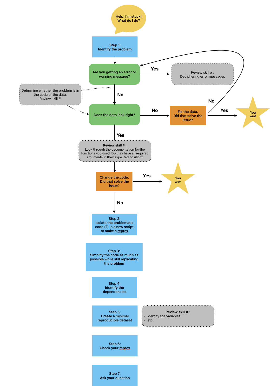
Since code first aid was not enough to solve this problem, it looks like it’s time to ask for help using a reprex.

Making a reprex

Simplify the code

When asking someone else for help, it is important to simplify your code as much as possible to make it easier for the helper to understand what is wrong. Simplifying code helps to reduce frustration and overwhelm when debugging an error in a complicated script. The more that we can make the process of helping easy and painless for the helper, the more likely that they will take the time to help.

Let’s look at all the code that Mickey has written so far.

Callout

Depending on how closely you have been following the lesson and which challenges you have attempted, your script may not look exactly like Mickey’s. That’s okay!

R

# Load packages and data
library(ggplot2)
library(dplyr)
rodents <- read.csv("data/surveys_complete_77_89.csv")

# XXX ADD PETER'S EPISODE CODE HERE

## Filter to only rodents
rodents <- rodents %>% filter(taxa == "Rodent")

# Visualize sex by species
ggplot(rodents, aes(x = species, fill = sex))+
  geom_bar()

# Subset to species and sexes of interest
rodents_subset <- rodents %>%
  filter(species == c("ordii", "spectabilis"),
         sex == c("F", "M"))

# Add common names
# common_names <- data.frame(species = unique(rodents_subset$species), common_name = c("Ord's", "Banner-tailed"))
# common_names # oops, this looks wrong!
common_names <- data.frame(species = sort(unique(rodents_subset$species)), common_name = c("Ord's", "Banner-Tailed"))
common_names
rodents_subset <- left_join(rodents_subset, common_names)

# Add a date column
# rodents_subset <- rodents_subset %>%
#   mutate(date = lubridate(paste(year, month, day, sep = "-"))) # that didn't work!

rodents_subset <- rodents_subset %>%
  mutate(date = lubridate::ymd(paste(year, month, day, sep = "-")))

# Predict weight by species and sex, and make a plot
weight_model <- lm(weight ~ common_name + sex, data = rodents_subset)
summary(weight_model) 
rodents_subset %>%
  ggplot(aes(y = weight, x = common_name, fill = sex)) +
  geom_boxplot() # wait, why does this look weird?

# Investigate
table(rodents_subset$sex, rodents_subset$species)
table(rodents$sex, rodents$species)

Wow, that’s a lot! Mickey’s code also contains explanatory comments (which are great, but they may or may not be relevant to the problem at hand), and when their code threw errors, they sometimes kept the old code, commented out, for future reference.

Create a new script

To make the task of simplifying the code less overwhelming, let’s create a separate script for our reprex. This will let us experiment with simplifying our code while keeping the original script intact.

Let’s create and save a new, blank R script and give it a name, such as “reprex-script.R”

Creating a new R script

There are several ways to make an R script:

File > New File > R Script
Click the white square with a green plus sign at the top left corner of your RStudio window
Use a keyboard shortcut: Cmd + Shift + N (on a Mac) or Ctrl + Shift + N (on Windows)

We’re going to start by copying over all of our code, so we have an exact copy of the full analysis script.

R

# Minimal reproducible example script
# Load packages and data
library(ggplot2)
library(dplyr)
rodents <- read.csv("data/surveys_complete_77_89.csv")

# XXX ADD PETER'S EPISODE CODE HERE

## Filter to only rodents
rodents <- rodents %>% filter(taxa == "Rodent")

# Visualize sex by species
ggplot(rodents, aes(x = species, fill = sex))+
  geom_bar()

# Subset to species and sexes of interest
rodents_subset <- rodents %>%
  filter(species == c("ordii", "spectabilis"),
         sex == c("F", "M"))

# Add common names
# common_names <- data.frame(species = unique(rodents_subset$species), common_name = c("Ord's", "Banner-tailed"))
# common_names # oops, this looks wrong!
common_names <- data.frame(species = sort(unique(rodents_subset$species)), common_name = c("Ord's", "Banner-Tailed"))
common_names
rodents_subset <- left_join(rodents_subset, common_names)

# Add a date column
# rodents_subset <- rodents_subset %>%
#   mutate(date = lubridate(paste(year, month, day, sep = "-"))) # that didn't work!

rodents_subset <- rodents_subset %>%
  mutate(date = lubridate::ymd(paste(year, month, day, sep = "-")))

# Predict weight by species and sex, and make a plot
weight_model <- lm(weight ~ common_name + sex, data = rodents_subset)
summary(weight_model) 
rodents_subset %>%
  ggplot(aes(y = weight, x = common_name, fill = sex)) +
  geom_boxplot() # wait, why does this look weird?

# Investigate
table(rodents_subset$sex, rodents_subset$species)
table(rodents$sex, rodents$species)

Now, we will follow a process: 1. Identify the symptom of the problem. 2. Remove a piece of code to make the reprex more minimal. 3. Re-run the reprex to make sure the reduced code still demonstrates the problem–check that the symptom is still present.

In this case, the problem is that we are missing rows in rodents_subset that were present in rodents and should not have been removed!

Let’s start by identifying pieces of code that we can probably remove. A good start is to look for lines of code that do not create variables for later use, or lines that add complexity to the analysis that is not relevant to the problem at hand.

For starters, we can certainly remove the broken code that we commented out earlier! Also, adding a date column is not directly relevant to the current problem. Let’s go ahead and remove those pieces of code. Now our script looks like this:

R

# Minimal reproducible example script
# Load packages and data
library(ggplot2)
library(dplyr)
rodents <- read.csv("data/surveys_complete_77_89.csv")

# XXX ADD PETER'S EPISODE CODE HERE

## Filter to only rodents
rodents <- rodents %>% filter(taxa == "Rodent")

# Visualize sex by species
ggplot(rodents, aes(x = species, fill = sex))+
  geom_bar()

# Subset to species and sexes of interest
rodents_subset <- rodents %>%
  filter(species == c("ordii", "spectabilis"),
         sex == c("F", "M"))

# Add common names
common_names <- data.frame(species = sort(unique(rodents_subset$species)), common_name = c("Ord's", "Banner-Tailed"))
common_names
rodents_subset <- left_join(rodents_subset, common_names)

# Predict weight by species and sex, and make a plot
weight_model <- lm(weight ~ common_name + sex, data = rodents_subset)
summary(weight_model) 
rodents_subset %>%
  ggplot(aes(y = weight, x = common_name, fill = sex)) +
  geom_boxplot() # wait, why does this look weird?

# Investigate
table(rodents_subset$sex, rodents_subset$species)
table(rodents$sex, rodents$species)

When we run this code, we can confirm that it still demonstrates our problem. There are still many rows missing from rodents_subset.

We’ve made progress on minimizing our code, but we still have a ways to go. This script is still pretty long! Let’s identify more pieces of code that we can remove.

Minimizing code

Which other lines of code can you remove to make this script more minimal? After removing each one, be sure to re-run the code to make sure that it still reproduces the error. :::solution - [Peter’s episode code] - Visualizing sex by species (ggplot) can be removed because it generates a plot but does not create any variables that are used later. - Filtering to only rodents can be removed because later we filter to only two species in particular - Adding common names can be removed because we didn’t actually use those common names. This one is tricky because technically we did use the common names in the rodents_subset plot. But is that plot really necessary? We can still demonstrate the problem using the table() lines of code at the end. Also, we could still make the equivalent plot using the species column instead of the common_name column, and it would demonstrate the same thing! - The weight model and the summary can be removed

A totally minimal script would look like this:

R

rodents <- read.csv("data/surveys_complete_77_89.csv")

rodents_subset <- rodents %>%
  filter(species == c("ordii", "spectabilis"),
         sex == c("F", "M"))

table(rodents_subset$sex, rodents_subset$species)
table(rodents$sex, rodents$species)

:::

Great, now we have a totally minimal script!

However, we’re not done yet.

The problem area is not enough

Let’s suppose that Mickey has created the minimal problem area script shown above. They email this script to Remy so that Remy can help them debug the code.

Remy opens up the script and tries to run it on their computer, but it doesn’t work. - What do you think will happen when Remy tries to run the code from this reprex script? - What do you think Mickey should do next to improve the minimal reproducible example?

We haven’t yet included enough code to allow a helper, such as Remy, to run the code on their own computer. If Remy tries to run the reprex script in its current state, they will encounter errors because they don’t have access to the same R environment that Mickey does.

Include dependencies

R code consists primarily of functions and variables. In order to make our minimal examples truly reproducible, we have to give our helpers access to all the functions and variables that are necessary to run our code.

First, let’s talk about functions. Functions in R typically come from packages. You can access them by loading the package into your environment.

To make sure that your helper has access to the packages necessary to run your reprex, you will need to include calls to library() for whichever packages are used in the code. For example, if your code uses the function lmer from the lme4 package, you would have to include library(lme4) at the top of your reprex script to make sure your helper has the lme4 package loaded and can run your code.

Callout

Some packages, such as {base} and {stats}, are loaded in R by default, so you might not have realized that a lot of functions, such as dim, colSums, factor, and length actually come from those packages!

You can see a complete list of the functions that come from the {base} and {stats} packages by running library(help = "base") or library(help = "stats").

Let’s do this for our own reprex. We can start by identifying all the functions used, and then we can figure out where each function comes from to make sure that we tell our helper to load the right packages.

The first function used in our example is ggplot(), which comes from the package ggplot2. Therefore, we know we will need to add library(ggplot2) at the top of our script.

The function geom_boxplot() also comes from ggplot2. We also used the function table(). Running ?table tells us that the table function comes from the package {base}, which is automatically installed and loaded when you use R–that means we don’t need to include library(base) in our script.

Our reprex script now looks like this:

R

# Mickey's reprex script

# Load necessary packages to run the code
library(ggplot2)

rodents_subset %>%
  ggplot(aes(y = weight, x = common_name, fill = sex)) +
  geom_boxplot() # wait, why does this look weird?

WARNING

Warning: Removed 35 rows containing non-finite outside the scale range
(`stat_boxplot()`).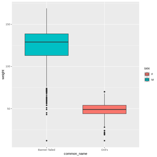

R

# Investigate
table(rodents_subset$sex, rodents_subset$species)

OUTPUT


    ordii spectabilis
  F   350           0
  M     0         626

R

table(rodents$sex, rodents$species)

OUTPUT


    albigula eremicus flavus fulvescens fulviventer harrisi hispidus
          62       14     15          0           0     136        2
  F      474      372    222         46           3       0       68
  M      368      468    302         16           2       0       42

    leucogaster maniculatus megalotis merriami ordii penicillatus  sp.
             16           9        33       45     3            6   10
  F         373         160       637     2522   690          221    4
  M         397         248       680     3108   792          155    5

    spectabilis spilosoma taylori torridus
             42       149       0       28
  F        1135         1       0      390
  M        1232         1       3      441

Installing vs. loading packages

But what if our helper doesn’t have all of these packages installed? Won’t the code not be reproducible?

Typically, we don’t include install.packages() in our code for each of the packages that we include in the library() calls, because install.packages() is a one-time piece of code that doesn’t need to be repeated every time the script is run. We assume that our helper will see library(specialpackage) and know that they need to go install “specialpackage” on their own.

Technically, this makes that part of the code not reproducible! But it’s also much more “polite”. Our helper might have their own way of managing package versions, and forcing them to install a package when they run our code risks messing up our workflow. It is a common convention to stick with library() and let them figure it out from there.

Which packages are essential?

In each of the following code snippets, identify the necessary packages (or other code) to make the example reproducible.

[Example (including an ambiguous function: dplyr::select() is a good one because it masks plyr::select())]
[Example where you have to look up which package a function comes from]
[Example with a user-defined function that doesn’t exist in any package]

This exercise should take about 10 minutes. :::solution FIXME

:::::::::::::::::::::::::::::::::::::::::::

Including library() calls will definitely help Remy run the code. But this code still won’t work as written because Remy does not have access to the same objects that Mickey used in the code.

The code as written relies on rodents_subset, which Remy will not have access to if they try to run the code. That means that we’ve succeeded in making our example minimal, but it is not reproducible: it does not allow someone else to reproduce the problem!

[Transition to minimal data episode]

Reflection

Let’s take a moment to reflect on this process.

What’s one thing you learned in this episode? An insight; a new skill; a process?
What is one thing you’re still confused about? What questions do you have?

This exercise should take about 5 minutes.

Key Points

Making a reprex is the next step after trying code first aid.
In order to make a good reprex, it is important to simplify your code
Simplify code by removing parts not directly related to the question
Give helpers access to the functions used in your code by loading all necessary packages

Minimal Reproducible Code

Overview

Questions

Objectives

XXX updateme

OUTPUT

OUTPUT

OUTPUT

R

R

R

OUTPUT

Applying code first aid

R

OUTPUT

R

OUTPUT

R

ERROR

Applying code first aid, part 2

Applying code first aid, part 2 (extra challenge)

R

WARNING

R

R

OUTPUT

R

WARNING

R

OUTPUT

R

OUTPUT

Making a reprex

Simplify the code

Callout

R

Create a new script

Creating a new R script

R

R

Minimizing code

R

The problem area is not enough

Include dependencies

Callout

R

WARNING

R

OUTPUT

R

OUTPUT

Installing vs. loading packages

Which packages are essential?

Reflection

Key Points