
Training Models in SageMaker: PyTorch Example
Last updated on 2026-11-02 | Edit this page
Overview
Questions
- When should you consider using a GPU instance for training neural networks in SageMaker, and what are the benefits and limitations?
- How does SageMaker handle data parallelism and model parallelism, and which is suitable for typical neural network training?
Objectives
- Preprocess the Titanic dataset for efficient training using PyTorch.
- Save and upload training and validation data in
.npzformat to S3. - Understand the trade-offs between CPU and GPU training for smaller datasets.
- Train a PyTorch model as a SageMaker training job and compare CPU and GPU instance types on time and cost.
- Differentiate between data parallelism and model parallelism, and determine when each is appropriate in SageMaker.
Open the notebook from:
/ML_with_AWS_SageMaker/notebooks/07_Training-models-in-SageMaker-notebooks-part2.ipynb.
Select the conda_pytorch kernel.
The same pattern with a neural network
The previous episode tested an XGBoost script on the notebook and then launched it as a managed training job. This episode follows the same pattern with a small PyTorch neural network on the same Titanic prediction task. Keeping the data and the task fixed means that what changes between runs is only the instance, so CPU and GPU can be compared on their own.
A GPU costs about six times more per hour than the CPU instance, so it has to train the model at least six times faster to be worth it. For a network this small, most of a job’s time is startup, not training. We run the same job on both and read the bills. Then we try two instances instead of one, and see why that does not halve the time.
Setup
We use the same controller notebook, SageMaker role, S3 bucket and Titanic files as in the XGBoost episode. The notebook prepares and uploads the data, then launches the training job on the instance we choose.
PYTHON
import boto3
import pandas as pd
import sagemaker
from sagemaker import get_execution_role

# Initialize the SageMaker role (will reflect notebook instance's policy)
role = sagemaker.get_execution_role()
print(f'role = {role}')

# Initialize an S3 client to interact with Amazon S3, allowing operations like uploading, downloading, and managing objects and buckets.
s3 = boto3.client('s3')

# Define the S3 bucket that we will load from
bucket_name = 'sinkorswim-doejohn'  # replace with your S3 bucket name

# Define train/test filenames
train_filename = 'titanic_train.csv'
test_filename = 'titanic_test.csv'
PYTHON
region = boto3.Session().region_name  # inherited from the notebook instance; do not hard-code a region
session = sagemaker.Session()
sagemaker_client = session.sagemaker_client  # low-level boto3 client; describe_training_job() below uses it
print(f"region = {region}")
Work in the Titanic folder beside the lesson clone, with the helper module on the path, and record which instance this notebook runs on so that runtimes can be compared.
PYTHON
# The Titanic project folder from the S3 episode, beside the lesson clone: downloads and outputs land here, not in the repository
!mkdir -p /home/ec2-user/SageMaker/titanic
%cd /home/ec2-user/SageMaker/titanic
import sys
sys.path.insert(0, "/home/ec2-user/SageMaker/ML_with_AWS_SageMaker/scripts")
import helpers
PYTHON
notebook_instance_name = 'SinkOrSwim-DoeJohn' # replace with your notebook instance name

local_instance_info = helpers.get_notebook_instance_info(notebook_instance_name, region)
local_instance = local_instance_info['InstanceType']
local_instance
If you are starting from a fresh notebook instance, download the Titanic CSVs from S3 again.
Training a neural network with SageMaker
The prediction task is unchanged, and only the training framework is different. So the attention goes to the PyTorch training workflow and to what the choice of instance does to runtime and cost.
Preparing the data
Unlike the XGBoost script, this PyTorch script expects features and
labels already processed into NumPy arrays. We prepare those arrays
once, save the training and validation sets as .npz files,
and upload them to S3. That keeps preprocessing out of the managed job,
and every run we compare trains on the same inputs.
Open ML_with_AWS_SageMaker/scripts/train_nn.py in the
file browser and read it before going on; it is short. Three things to
find: TitanicNet, a three-layer network with 7 inputs and
one output; the training loop in train(), which prints
validation:accuracy = ... once per hundred epochs (the
hyperparameter-tuning episode’s metric regex reads that line); and the
last lines, which save the model to /opt/ml/model inside a
job and to the working directory otherwise, the same trick as
train_xgboost.py. Questions now are cheaper than questions
once it is running on a billed instance.
We reuse the preprocess_data() function from the
lesson’s scripts/train_nn.py instead of retyping the
preprocessing here: the same function will later be applied to the test
set, so train and test are transformed identically. It returns the
fitted StandardScaler, and we save it with
joblib so the next episode can load it.
Load the Titanic CSV, run it through the script’s
preprocess_data, split off a validation set, and save the
arrays and the scaler. The training script reads these files; the scaler
is kept so test data can later be transformed the same way.
PYTHON
import numpy as np
import joblib
from sklearn.model_selection import train_test_split
from train_nn import preprocess_data

# Load and preprocess the Titanic dataset: encode Sex/Embarked, fill missing Age/Fare, standardize features
df = pd.read_csv(train_filename)
X, y, scaler = preprocess_data(df)   # scaler is fit on the training data only

# Split the data
X_train, X_val, y_train, y_val = train_test_split(X, y, test_size=0.2, random_state=42)

# Save the preprocessed data (and the fitted scaler) to our local jupyter environment
np.savez('train_data.npz', X_train=X_train, y_train=y_train)  # .npz = several numpy arrays in one compressed file, read back by key
np.savez('val_data.npz', X_val=X_val, y_val=y_val)
joblib.dump(scaler, 'scaler.joblib')  # keep the fitted scaler: the test set must be transformed with these same means/stds, never refit
print(X_train.shape, X_val.shape)
Next, we will upload our compressed files (and the scaler) to our S3
bucket. Storage is $0.023 per GB per month; a preprocessed
copy of a small dataset costs nothing worth counting.
PYTHON
train_file = "train_data.npz"  # Local file path in your notebook environment
val_file = "val_data.npz"  # Local file path in your notebook environment
scaler_file = "scaler.joblib"

# Upload the training and validation files (and the scaler) to the bucket root
for f in [train_file, val_file, scaler_file]:
    s3.upload_file(f, bucket_name, f)

print("Files successfully uploaded to S3.")
Check the training script
Before launching a managed job, we run 100 epochs on the controller notebook as a short test. It checks the data paths and the training code and gives a rough time per epoch. It is only a local test. The runs we compare are launched as separate SageMaker jobs.
PYTHON
import torch
import time as t # Measure training time locally

epochs = 100          # a short test run
learning_rate = 0.001

start_time = t.time()
%run /home/ec2-user/SageMaker/ML_with_AWS_SageMaker/scripts/train_nn.py --train train_data.npz --val val_data.npz --epochs {epochs} --learning_rate {learning_rate}
local_elapsed = t.time() - start_time   # kept for the estimate below
print(f"Local training time: {local_elapsed:.2f} seconds, instance_type = {local_instance}")
The network as a SageMaker training job
Now we submit a 1,000-epoch run as a SageMaker job. Its compute is
chosen on the estimator, independently of the notebook that launches it.
The first run uses the same ml.m5.large CPU instance as the
XGBoost job, so there is a baseline before trying a GPU.
A GPU is not necessarily worth it for this data. The CPU instance
costs $0.115 an hour and an ml.g4dn.xlarge GPU
instance $0.74 an hour on the Instances
for ML page. The GPU would have to save enough time to make up that
difference, and the model may be too small to keep it busy. We measure
it instead of assuming the more powerful hardware is the better
choice.
Cost tracking
As in the XGBoost episode, every training job needs its own tags: a
job does not inherit the notebook instance’s tags, and an untagged job
is anonymous on the bill. Define them once here and pass
tags=job_tags to every estimator below.
PYTHON
name = "DoeJohn" # replace with your name
project = "SinkOrSwim"   # your challenge: WattBot2026, BadgerScribe, BadgerCode, BrainDecoding, PoisonedWell or SnapshotWI; SinkOrSwim is the workshop itself
purpose = "Training"        # one of: Storage, Notebook, Training, Tuning, Inference

job_tags = [
    {"Key": "Name", "Value": name},
    {"Key": "Project", "Value": project},
    {"Key": "Purpose", "Value": purpose},
]
helpers.check_launch(job_tags)   # the account's rules, checked here first: AWS's own refusal does not say which rule
print(f"Name: {name}, Project: {project}, Purpose: {purpose}")
Estimating a training job before you launch it
Every job in this lesson gets an estimate written down before
fit(), a rough figure for how long it will run and what it
will cost. There are two ways to make it, and which one applies depends
on the size of the model. For a model this small, timing a short test
run is more useful than counting the arithmetic, so the measured time
comes first and the counted arithmetic, which the larger models later in
the workshop need, after it.
Small models: time a short run and scale it. The 100-epoch test gives a time per epoch. Each epoch costs the same as the last, and the script trains on all the rows in one step per epoch, so training time scales with epochs and with rows. Scale the measured time to 1,000 epochs, then add the two or three minutes of container startup and data download, which are billed and are most of the bill for a job this small. The result is not exact, because the notebook and the training instance are different machines, but it says whether the job will cost cents or dollars:
PYTHON
local_seconds_per_epoch = local_elapsed / epochs                 # from the short run above: its wall-clock over its 100 epochs
planned_epochs = 1000
startup_minutes = 3                                            # container pull + data download, billed; the same for every job
rate = 0.115                                                   # $/hour, ml.m5.large, from the Instances for ML page

train_minutes = local_seconds_per_epoch * planned_epochs / 60
estimate = (train_minutes + startup_minutes) / 60 * rate
print(f"{local_seconds_per_epoch * 1000:.1f} ms per epoch locally -> {train_minutes:.1f} min of training for {planned_epochs} epochs")
print(f"estimate: {train_minutes + startup_minutes:.0f} min billed, about ${estimate:.3f} on ml.m5.large")
Expect a couple of minutes of training plus two or three of startup:
about a cent. (The ml.t3.medium notebook is slower than the
ml.m5.large the job runs on, so the training part of the
estimate is high. Our run billed 2.7 minutes in total,
$0.005.) If the planned run has ten times the rows,
multiply the training minutes by ten; the startup does not change.
Large models: count the arithmetic. From a few hundred million parameters up, the training arithmetic takes longer than the job’s startup, so the arithmetic is the cost, and it can be counted before any instance exists. The work is counted in floating-point operations, FLOPs, one multiply or one add, and a GPU’s speed in FLOPS, operations per second, about 70 trillion for an A10G. Training one token through a dense network or a transformer costs about 6 FLOPs per parameter, 2 for the forward pass and 4 for the backward one. Multiply by parameters, examples and epochs for the count, and divide by the speed the GPU reaches, about a quarter of its data-sheet peak in practice. It is a scale estimate, not a runtime prediction:
FLOPs       = 6 × parameters × examples × tokens per example × epochs
GPU-seconds = FLOPs ÷ (GPU peak FLOPS × 0.25)
cost        = GPU-hours × instance price per hour + startup
On TitanicNet the arithmetic comes out as a fraction of
a second, which is why timing a short run is the method to use for
it:
PYTHON
from train_nn import TitanicNet
n_params = sum(p.numel() for p in TitanicNet().parameters())   # the network's weights and biases: how big the model is
n_examples = len(np.load("train_data.npz")["X_train"])          # one example = one passenger, a row of 7 numbers; 569 of them after the validation split
tokens_per_example = 1                                          # the network reads a whole row in one step, so a row is one token
flops = 6 * n_params * n_examples * tokens_per_example * planned_epochs
print(f"{n_params:,} parameters x {n_examples} examples x {planned_epochs} epochs = {flops:.1e} FLOPs")
print(f"on an A10G at a quarter of 70 TFLOPS: {flops / (70e12 * 0.25):.4f} seconds of arithmetic; the bill is the startup")
The same rule, in helpers.estimate_training_cost, picks
an instance and prints the time, cost and max_run for any
model size. It only earns its keep once the arithmetic outweighs the
startup, from a few hundred million parameters up, which is where the
fine-tuning episode uses it on a 3-billion-parameter model. Its four
inputs are the four numbers in the formula, and what each one is depends
on the data:
-
params_billions: every parameter in the model, in billions.TitanicNethas 2,625, which is 0.0000026; a BERT-base text classifier has 110 million, 0.11. -
examples: one example is one training item, whatever the model takes in at a time. A passenger’s row here; one tweet, one abstract, one document for a text model; one page image in the fine-tuning episode. -
tokens_per_example: how many units the model processes for one item, which is what the arithmetic scales with. A row throughTitanicNetis one step, so 1. A text model works in tokens, about 1.3 per English word: a tweet is 40, an abstract 256, a short paper 2,000. An image through a vision transformer is one token per patch, 196 for a 224 × 224 image in 16 × 16 patches. -
epochs: passes over the whole set.
The three data numbers multiply to the tokens the model trains on. Here it is on a run that does need the rule: a BERT-sized text classifier trained from scratch on a million abstracts, three passes:
PYTHON
helpers.estimate_training_cost(   # the semicolon at the end keeps Jupyter from also displaying the dictionary the function returns
    params_billions=0.125,      # a BERT-base-sized model, 125 million parameters
    examples=1_000_000,         # a million abstracts
    tokens_per_example=256,     # 190 words per abstract, about 256 tokens
    epochs=3,                   # three full training passes over all abstracts
);
Each line:
- tokens: examples × tokens per example × epochs. 768 million tokens is the amount of work; everything below is derived from it.
-
memory: 16 bytes per parameter for full training
(the weight, its 32-bit master copy, its gradient and the optimizer’s
two running averages, in the fine-tuning episode’s table) is 2 GB for
125 million parameters, plus 4 GB the helper allows for activations: 6
GB. The cheapest GPU on the lesson’s list with that much memory is the
ml.g6.xlarge, one L4 with 24 GB, so that is the instance the rest of the lines price. - compute: 6 FLOPs × 0.125e9 parameters × 768e6 tokens is 5.8e17; the helper multiplies by 1.5 because it assumes gradient checkpointing, which recomputes the forward pass during the backward one to save memory, giving 8.6e17. Divided by a quarter of the L4’s 121 TFLOPS peak, 30 trillion a second, that is 28,500 seconds: 7.9 GPU-hours.
- wall-clock: the GPU-hours on one GPU, plus the 10 minutes of startup the helper assumes for a job this size.
-
cost: the wall-clock hours at the instance’s price,
$1.13an hour, so about$9a run. The second figure is the same times the number of runs, one here; the hyperparameter-tuning episode is where that multiplier bites. -
max_run: twice the wall-clock estimate, in seconds,
ready to paste into the estimator. A job that runs past this is killed,
so a hung run costs at most
$18, not a week.
The function also returns the same numbers as a dictionary, so a
notebook can use max_run_seconds and
instance_type directly, with no copying from the
printout.
What training a language model would cost
Run the same function on two sizes a project might be tempted by: a 1-billion-parameter model and a 7-billion one, each trained from scratch on a million papers, one pass. Nothing is launched; the function only does the arithmetic.
PYTHON
helpers.estimate_training_cost(
    params_billions=1,          # a 1B model, the size of the smallest open-weight language models
    examples=1_000_000,         # a million papers
    tokens_per_example=2000,    # 1,500 words per paper, about 2,000 tokens
    epochs=1,                   # one full training pass over all papers
);
PYTHON
helpers.estimate_training_cost(
    params_billions=7,          # a 7B model, the size most "small" open-weight LLMs are
    examples=1_000_000,         # the same million papers
    tokens_per_example=2000,    # 1,500 words per paper, about 2,000 tokens
    epochs=1,                   # one full training pass over all papers
);
Read the two against the 125M run above. The 1B model still fits on
the cheapest GPU, but the arithmetic is 165 GPU-hours: a week of
wall-clock on one GPU, $187, and a max_run of
330 hours, which the account refuses, since no job may run longer than
48 hours. A run like that has to be split into checkpointed jobs of a
day or two each, or moved to a four-GPU box, an
ml.g6e.12xlarge, which finishes in about 14 hours for about
$180, and which the class account does not allow. The 7B
model no longer fits on one GPU at all: 116 GB of weights, gradients and
optimizer state need the four-GPU ml.g6e.12xlarge at
$13 an hour, four days of it, $1,270 for one
pass over two billion tokens. And two billion tokens is a small corpus;
the models on Bedrock were trained on thousands of times more.
That is why nothing in this lesson trains a language model. What the lesson does instead is in the fine-tuning episode, LoRA on a 3-billion-parameter model, which trains tens of millions of adapter parameters on 251 pages for about a dollar, and the RAG episodes, which use a trained model through Bedrock by the token. The function is for the day a project asks for more: run it first, and the number says whether the run is a job, a grant line, or something to do differently.
Estimate your own first run
Take the model you expect to train for your own project or challenge, or the biggest one you have trained before, and estimate its first SageMaker run before you ever launch one. You need four numbers:
-
Parameters. For a model you have in PyTorch,
sum(p.numel() for p in model.parameters()); for a model card, it is in the name (-7B,-125M). - Examples and tokens per example. Rows for tabular data, sequence length for text, one token per patch for an image through a vision transformer (196 for a 224 × 224 image in 16 × 16 patches); for a convolutional network use the FLOPs-per-image figure from its paper instead of the 6 × parameters rule.
- Epochs. Small data usually takes three to five passes, large corpora one to three; the number is a budget, not a given.
- Instance. From the Instances for ML page, or let the helper pick the cheapest that fits.
If the FLOPs come out below 1e15, time a short run instead and say
what you would measure. Write the estimate down with the
max_run you would set, and keep it: the first bill goes
next to it.
There is no single answer; the solution is the written estimate. One
worked example for scale: a 7B language model fully fine-tuned on 50,000
documents of 2,000 tokens for 3 epochs is 6 × 7e9 × 3e8 = 1.3e19 FLOPs,
45 GPU-hours on A100s, about $140 a run; the fine-tuning
episode works that one through. A 10-million-parameter network on
100,000 rows for 20 epochs is 1.2e14 FLOPs: below the line, so time a
short run and scale it, and expect the startup minutes to dominate.
We’ll also bring back the job_cost_report() helper from
the previous episode, plus the hourly rates of the instances we’re about
to use.
PYTHON
def job_cost_report(job_name: str, price_per_hour: float):
    desc = session.sagemaker_client.describe_training_job(TrainingJobName=job_name)  # the job record the console shows
    if "BillableTimeInSeconds" not in desc:   # the job has not finished: no bill yet
        print(f"{job_name}: status {desc['TrainingJobStatus']}; billable time and the model path appear once it is Completed")
        return desc
    n = desc["ResourceConfig"]["InstanceCount"]
    billable = desc["BillableTimeInSeconds"] * n   # container pull to model upload, charged per instance
    wall = (desc["TrainingEndTime"] - desc["CreationTime"]).total_seconds()   # from the launch request to the end, including unbilled provisioning
    print(f"{job_name}: status {desc['TrainingJobStatus']}, wall-clock {wall/60:.1f} min, billable {billable/60:.1f} min on {n} instance(s), cost ${billable/3600*price_per_hour:.3f} at ${price_per_hour}/h")
    print(f"    model: {desc['ModelArtifacts']['S3ModelArtifacts']}")   # the model.tar.gz this job uploaded to output_path
    return desc

# us-east-1 on-demand rates (2026-10-16); check the instances page for your region
prices = {"ml.m5.large": 0.115, "ml.g4dn.xlarge": 0.74}
Set up the estimator for a longer run: the epochs, the instance,
where the output goes, and a two-hour max_run cap. If the
launch is refused with an AccessDeniedException ending in
explicit deny, the account’s checks are the cause: a
missing tag, an instance type outside the lesson’s list, or a resource
kind the lesson never creates; the first training episode’s callout
If the launch is refused says what to look at.
PYTHON
from sagemaker.pytorch import PyTorch
from sagemaker.inputs import TrainingInput

epochs = 1000          # more epochs now that the script is known to work
instance_count = 1
instance_type = "ml.m5.large"
output_path = f's3://{bucket_name}/output_nn/' # this folder will auto-generate if it doesn't exist already

# The runtime cap, in seconds: SageMaker stops the job and releases the instance when it is reached. Set it a little above the estimate;
# the estimate here is three or four minutes, so 20 minutes leaves room for a slow container pull without letting a hung job bill for hours.
max_run = 20*60 # 20 minutes

# Define the PyTorch estimator and pass hyperparameters as arguments
pytorch_estimator = PyTorch(
    base_job_name=f"{notebook_instance_name}-nn",   # who + which model; SageMaker appends a timestamp to make each job name unique
    max_run=max_run, # in seconds; always include (max 48 hours)
    entry_point="/home/ec2-user/SageMaker/ML_with_AWS_SageMaker/scripts/train_nn.py",  # copied into the container and run there
    role=role,
    tags=job_tags,  # per job; nothing is inherited from the notebook instance
    instance_type=instance_type, # with this small dataset, we don't necessarily need a GPU for fast training.
    instance_count=instance_count,
    # framework_version + py_version pick the prebuilt PyTorch training image the job runs in
    framework_version="2.3",  # if fit() fails with an image error, check available versions with: sagemaker.image_uris.retrieve("pytorch", region, version="2.3", py_version="py311", image_scope="training", instance_type="ml.m5.large")
    py_version="py311",
    output_path=output_path,
    sagemaker_session=session,
    hyperparameters={  # passed to train_nn.py as command-line flags: --train ... --epochs 1000 ...
        "train": "/opt/ml/input/data/train/train_data.npz",  # SageMaker will mount this path
        "val": "/opt/ml/input/data/val/val_data.npz",        # SageMaker will mount this path
        "epochs": epochs,
        "learning_rate": learning_rate
    }
)

# Define input paths: each TrainingInput is a channel; its S3 object is copied to /opt/ml/input/data/<channel>/ in the container
# content_type is a label only; our script reads the file itself
train_input = TrainingInput(f"s3://{bucket_name}/train_data.npz", content_type="application/x-npz")
val_input = TrainingInput(f"s3://{bucket_name}/val_data.npz", content_type="application/x-npz")

# Start the training job and time it
start = t.time()
pytorch_estimator.fit({"train": train_input, "val": val_input})
end = t.time()

print(f"Runtime for training on SageMaker: {end - start:.2f} seconds, instance_type: {instance_type}, instance_count: {instance_count}")
PYTHON
desc_cpu = job_cost_report(pytorch_estimator.latest_training_job.name, prices[instance_type])For a job this small, almost all of the billable minutes are startup.
The same job on a GPU instance
A second job: the same script and the same data, with one change,
instance_type, from the ml.m5.large to a GPU
instance. A job runs on one instance type; to compare two, you launch
two jobs and read both records, which is what the cell at the end of
this section does with the earlier job’s desc_cpu and this
one’s desc_gpu.
Selecting a GPU Instance
For a small dataset like ours, we don’t strictly need a GPU, but for
larger datasets or more complex models, a GPU can reduce training time.
Here, we’ll select an ml.g4dn.xlarge instance, which
provides a single GPU and costs approximately $0.74/hour
(check Instances
for ML page for detailed pricing).
The script does not change
train_nn.py already picks the GPU when there is one and
moves the model and the tensors to it, which is why the same file runs
on both instance types:
PY
device = torch.device("cuda" if torch.cuda.is_available() else "cpu")
model = TitanicNet().to(device)
X_train, y_train = X_train.to(device), y_train.to(device)Will the GPU job be faster or cheaper?
We’re about to run the identical job on an
ml.g4dn.xlarge (one NVIDIA T4 GPU, about
$0.74/hour) instead of the ml.m5.large
($0.115/hour); both rates are from the Instances
for ML page. Before you run the cell:
- Predict which instance finishes first (total wall-clock, as
fit()reports it). - Predict which costs less for this job.
Then run the GPU job, call job_cost_report() for it, and
compute cost = rate x billable minutes for both runs. Were you right?
Explain the result.
PYTHON
instance_type = "ml.g4dn.xlarge"  # one NVIDIA T4 GPU; train_nn.py moves to it on its own via torch.cuda.is_available()
instance_count = 1

pytorch_estimator_gpu = PyTorch(
    base_job_name=f"{notebook_instance_name}-nn",
    max_run=max_run, # in seconds; always include (max 48 hours)
    entry_point="/home/ec2-user/SageMaker/ML_with_AWS_SageMaker/scripts/train_nn.py",
    role=role,
    tags=job_tags,
    instance_type=instance_type,
    instance_count=instance_count,
    framework_version="2.3",
    py_version="py311",
    output_path=output_path,
    sagemaker_session=session,
    hyperparameters={
        "train": "/opt/ml/input/data/train/train_data.npz",
        "val": "/opt/ml/input/data/val/val_data.npz",
        "epochs": epochs,
        "learning_rate": learning_rate
    }
)

start = t.time()
pytorch_estimator_gpu.fit({"train": train_input, "val": val_input})
end = t.time()
print(f"Runtime for training on SageMaker: {end - start:.2f} seconds, instance_type: {instance_type}, instance_count: {instance_count}")

desc_gpu = job_cost_report(pytorch_estimator_gpu.latest_training_job.name, prices[instance_type])

# The two jobs side by side: the ml.m5.large job from earlier (desc_cpu) and this one (desc_gpu); same script, same data, different instance_type
for label, d, rate in [("job on ml.m5.large (CPU)", desc_cpu, prices["ml.m5.large"]), ("job on ml.g4dn.xlarge (GPU)", desc_gpu, prices["ml.g4dn.xlarge"])]:
    billable_min = d["BillableTimeInSeconds"] / 60
print(f"{label}: billable {billable_min:.1f} min x ${rate}/h = ${billable_min/60*rate:.3f}")Typically the CPU run finishes about as fast or faster, and it is
several times cheaper. Both jobs spend roughly the same few minutes on
startup (pulling the container, downloading data; the unbilled wait for
an instance comes before that), and the GPU container is larger, so it
often takes a little longer to start. The actual training is a
few seconds on either instance: the network has about 2,600 parameters
and the whole training set is 569 rows, so each full-batch step is tiny
and the T4 sits almost idle, and the one-time CUDA initialization adds a
few seconds of its own. Startup dominates both bills, and the GPU bill
is about 6x higher per minute (0.74 / 0.115), so the GPU costs several
times more for no speedup. In our run the CPU job billed 2.6 minutes
($0.005) and the GPU job 3.7 minutes ($0.046):
slower, and nine times the price. The GPU job’s wall-clock was 8.6
minutes, because it first sat four and a half minutes in
Pending - Training job waiting for capacity; GPU instances
are in shorter supply than CPU ones, and the wait is not billed.
A GPU is worth it when the per-step work is large enough to keep it
busy: bigger models, bigger batches, or datasets of hundreds of MB and
up. If you ever do need more GPU than a g4dn.xlarge, the
next sensible step is an ml.g5.xlarge
(~$1.41/hour), not a multi-GPU box.
More than one machine
When a run is too slow, the moves are in this order, and each one is tried before the next:
- A faster single device. The GPU exercise above. On the Instances for ML page that runs from the T4 through the A10G and L4 to the L40S, a fivefold range of speed at a twofold range of price, with no change to the script.
-
More devices in one box. A multi-GPU instance such
as
ml.g5.12xlargeorml.p4d.24xlarge. The GPUs share a link inside the machine, tens to hundreds of GB/s, so splitting a run across them loses little. - More than one instance. The same split across the network between instances, 10 to 400 Gb/s depending on the type, which is ten to a hundred times slower than the link inside a box. This is the last resort, for a run that will not fit one box or would take days on it.
Only the third needs more than a change of
instance_type, and on the class account it is the only form
available, since the instance list stops at one GPU per instance. The
rest of this section shows it on two ml.m5.large CPU
instances, where it costs cents, then estimates when it helps and shows
the setup for each kind of job.
What instance_count=2 does on its own
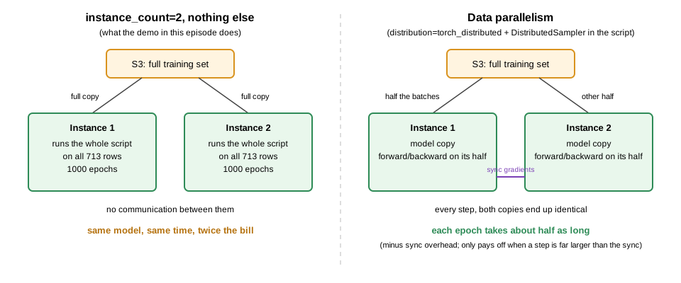
Setting instance_count=2 on an estimator makes SageMaker
start two instances and run the full training script on each of
them. Nothing is split:
-
TrainingInputdefaults todistribution="FullyReplicated", so every instance downloads the complete dataset. -
train_nn.pyhas no distributed code, so each instance trains its own independent copy of the model on all of the data for all 1000 epochs, and each saves a model. - SageMaker bills
BillableTimeInSeconds x InstanceCount.
So without a distribution strategy, two instances means the same job
twice, in parallel, at double the cost. There is nothing to launch to
see this; we ran it once while writing the episode, and the record is
what the bullets predict: the same 3.5 minutes of wall-clock as the
single-instance run, 5.5 billable minutes across the two instances,
$0.010, two CloudWatch log streams, algo-1 and
algo-2, each printing all 1000 epochs, and two identical
saved models. The job worth launching is below.
Data parallelism
To split one training run across two instances instead of running it
twice, the script needs three things train_nn.py does not
have, and the estimator needs one. scripts/train_nn_ddp.py
is train_nn.py with those three added; open the two side by
side; the three additions are marked 1, 2 and 3 in the comments.
-
Join the process group. The launcher starts one
copy of the script on each instance. The copies are numbered from zero,
and a copy’s number is its rank: with two instances,
one copy is rank 0 and the other rank 1, and the count of copies, 2, is
the world size. Each copy learns its own rank and the
world size from environment variables the launcher sets, and
setup_distributedreads them and callsinit_process_group, after which the copies can talk to each other. The rank is the only thing that differs between the copies, and everything below that has to differ between instances keys off it. With no launcher the function returns rank 0 of 1 and the script trains liketrain_nn.py. -
Shard the data. Each copy keeps the rows whose
index, counting from zero, leaves its rank as the remainder when divided
by the world size: rank 0 takes rows 0, 2, 4, … and rank 1 takes rows 1,
3, 5, …, which is
X_train[rank::world_size]. Half the training set each, no row seen twice, and the copies agree on the split without talking, because each one knows only its rank. -
Wrap the model in
DistributedDataParallel. After everyloss.backward(), DDP averages the gradients across the processes beforeoptimizer.step(), so both copies of the model take the same step and stay identical. That averaged gradient over two half-shards is the gradient over the whole set, which is why the result is one training run and not two. Only the copy with rank 0 prints the metrics and saves the model, since every copy holds the same weights and one file is enough; rank 0 is the conventional choice because every world has one.
On the estimator,
distribution={"mpi": {"enabled": True, "processes_per_host": 1}}
is what starts the processes: SageMaker launches the script on every
instance through MPI, which sets the rank and world-size variables the
script reads and lets the instances find each other by name.
(torch_distributed, the torchrun launcher, is
the same idea for GPU instances; the script handles either.) Everything
else is the single-instance estimator with
instance_count=2.
PYTHON
pytorch_estimator_ddp = PyTorch(
    base_job_name=f"{notebook_instance_name}-nn-ddp",
    max_run=max_run,
    entry_point="/home/ec2-user/SageMaker/ML_with_AWS_SageMaker/scripts/train_nn_ddp.py",   # the three additions, marked in the script
    role=role,
    tags=job_tags,
    instance_type="ml.m5.large",
    instance_count=2,
    distribution={"mpi": {"enabled": True, "processes_per_host": 1}},   # start one process per instance and connect them; without this, two copies again
    framework_version="2.3",
    py_version="py311",
    output_path=output_path,
    sagemaker_session=session,
    hyperparameters={
        "train": "/opt/ml/input/data/train/train_data.npz",
        "val": "/opt/ml/input/data/val/val_data.npz",
        "epochs": epochs,
        "learning_rate": learning_rate,
    },
)

start = t.time()
pytorch_estimator_ddp.fit({"train": train_input, "val": val_input})
print(f"Data-parallel run: {(t.time() - start) / 60:.1f} min wall-clock on 2 x ml.m5.large")
desc_ddp = job_cost_report(pytorch_estimator_ddp.latest_training_job.name, prices["ml.m5.large"])
Read the log before the bill. The two CloudWatch streams say
different things: each prints training on 285 of 569 rows
(or 284), and only algo-1 prints the epochs and saves the
model. That is the proof the work was split, not copied. The run’s final
numbers are close to the single-instance run but not identical (our run:
validation accuracy 0.818 against 0.804, validation loss 0.96 against
1.05): train_nn.py sets no random seed and
train_nn_ddp.py fixes one, so the two runs did not start
from the same weights, and a thousand Adam steps on a network that is
overfitting by epoch 300 turn any such difference into a visible one.
Two runs of train_nn.py differ from each other by as
much.
The comparison with the single-instance job, wall-clock and bill:
PYTHON
# Same script, same data, same epochs: one ml.m5.large (desc_cpu) against two with data parallelism (desc_ddp)
for label, d in [("1 x ml.m5.large", desc_cpu), ("2 x ml.m5.large, data parallel", desc_ddp)]:
    n = d["ResourceConfig"]["InstanceCount"]
    wall = (d["TrainingEndTime"] - d["CreationTime"]).total_seconds() / 60
    billable = d["BillableTimeInSeconds"] * n / 60
    print(f"{label:32s} wall-clock {wall:.1f} min, billable {billable:.1f} min on {n} instance(s), ${billable/60*prices['ml.m5.large']:.3f}")
Nothing was gained: the two-instance run took longer and cost twice
as much. Each step now ends with a gradient exchange between the two
machines, and that exchange has a fixed cost, a network round trip of
about a millisecond, plus the gradient’s bytes divided by the link’s
bandwidth. What it saves is the forward and backward pass over the 284
rows the other machine took, which for TitanicNet is
microseconds. The exchange is a per-step cost that is the same whether
the step is tiny or huge; here it is the whole step.
When a second machine helps
helpers.estimate_parallel_speedup puts numbers on that
for any model and any box, with the same assumptions as the cost
estimator: 6 FLOPs per parameter per token at a quarter of the GPU’s
peak, and a gradient of 4 bytes per trainable parameter exchanged once
per step over the slowest link in use. It does not overlap the exchange
with the computation, which real runs partly do, so its speedup is a
floor.
Its inputs differ from the cost estimator’s in one way. The cost
estimator takes the whole run, examples ×
tokens_per_example × epochs, because the bill
is the total work. This one takes a single step,
tokens_per_step, because the exchange happens once per step
and the speedup is the same for every step, so the length of the run
does not enter. A step is one batch, so tokens_per_step is
the batch size times the tokens per example, the same two numbers as the
cost estimator’s with the batch in place of the dataset. The 7B model
from the cost section, trained with a batch of 16 documents of 2,000
tokens each, three ways:
PYTHON
# Two single-GPU instances over the network: the class-account form of data parallelism
helpers.estimate_parallel_speedup(
    params_billions=7,
    tokens_per_step=16 * 2000,       # one step: a batch of 16 documents x 2,000 tokens each
    instance_type="ml.g6e.xlarge", instance_count=2,
);
PYTHON
# Four GPUs in one box, linked by PCIe
helpers.estimate_parallel_speedup(
    params_billions=7,
    tokens_per_step=16 * 2000,       # one step: a batch of 16 documents x 2,000 tokens each
    instance_type="ml.g6e.12xlarge",
);
PYTHON
# Eight GPUs in one box, linked by NVLink
helpers.estimate_parallel_speedup(
    params_billions=7,
    tokens_per_step=16 * 2000,       # one step: a batch of 16 documents x 2,000 tokens each
    instance_type="ml.p4d.24xlarge",
);
Read the three together. Two L40S instances over a 20 Gb/s network spend as long exchanging the 28 GB gradient as computing, so two machines finish in the same time as one and bill twice. Four L40S in one box over PCIe get 3.2 of the ideal 4. Eight A100s over NVLink get 7.8 of 8, which is why the big training boxes are built that way.
Data parallelism helps when each step’s computation is large next to the exchange, which means a big model, a big batch and a fast link, in that order of importance. Run the function before renting more than one device, and read the cost line: the speedup is what you buy, the cost ratio is what you pay for it.
Setting it up for each kind of job
A job has one instance type and one count; the count is how many of that type, and every instance gets the same script. What differs is how the work is split, which depends on what is running:
| Job | On the estimator | In the script | Data |
|---|---|---|---|
| Your own PyTorch script (this episode) |
distribution={"torch_distributed": {"enabled": True}}
on GPU instances, which starts one process per GPU;
{"mpi": {"enabled": True, "processes_per_host": 1}} on CPU
instances |
the three additions in train_nn_ddp.py: join the
process group, shard the rows, wrap the model in DDP; with a
DataLoader, a DistributedSampler does the
sharding |
one .npz per channel, FullyReplicated:
every instance downloads it and takes its shard |
Hugging Face Trainer (the fine-tuning episode) |
distribution={"torch_distributed": {"enabled": True}} |
nothing: Trainer detects the processes and does the
three things itself; per_device_train_batch_size is then
per GPU, so the effective batch is that times the device count |
as above |
| A model too large for one GPU’s memory | the same launcher |
fsdp= in the TrainingArguments (or
DeepSpeed), which shards the weights, gradients and optimizer state
across the GPUs so that a model too big for one fits; each GPU still
takes its own batch, so it is data parallelism with sharded state, for
memory and not for speed, and it only works inside one box or over a
fast network |
as above |
| Built-in XGBoost (the optional challenge in the previous episode) |
instance_count=N, no distribution
|
nothing: the algorithm trains across instances itself | the CSV split into several objects under one prefix, passed as
TrainingInput(prefix, distribution="ShardedByS3Key") so
each instance downloads only its share |
| Hyperparameter tuning |
instance_count=1 on the estimator; parallelism is
max_parallel_jobs on the tuner |
nothing | as for a single job |
Two things the table does not change. max_run is per
job, so a two-instance job with a 2-hour cap bills at most 4
instance-hours. And the account’s rules apply to every instance in the
job, so the instance type must be on the list and the tags are the job’s
tags.
- Startup dominates small jobs: Every SageMaker training job waits a minute or so for an instance (not billed), then spends one to three minutes on container pull and data download (billed) before the script runs; for a job whose script finishes in seconds, that overhead is the whole bill.
-
Estimate before you launch: for small models, time
a short run and scale it by epochs and rows, plus about three minutes of
startup; for large ones, 6 FLOPs per parameter per token, divided by a
quarter of the GPU’s peak.
helpers.estimate_training_costdoes the second; write the number down and compare it to the bill. -
GPU or CPU is a measurement: the same script on an
ml.g4dn.xlargewas slower and dearer than on anml.m5.largefor this network, because the step is too small to keep a GPU busy; the GPU pays when the model and batch are large. -
More than one machine is the last move: a faster
single device first, then more GPUs in one box, then more instances.
instance_count=2on its own runs the whole job twice and bills twice; data parallelism needsdistribution=on the estimator and, for your own script, three additions: join the process group, shard the rows, wrap the model in DDP. -
Parallelism pays when the step’s computation is large next
to the gradient exchange: big model, big batch, fast link.
helpers.estimate_parallel_speedupgives the speedup and the cost ratio before you rent the devices; on 569 rows of tabular data the measured result was 0.85x the speed at 2.4x the cost.