Data visualisation and scales
Last updated on 2026-05-26 | Edit this page
Overview
Questions
- How can I change the colour in my plots?
- How can I change the general look of my plot?
Objectives
- Use
scale_fill_xxx()andscale_colour_xxx()to change colours in your plot. - Use the
theme()functions to change the general look of your plot.
Motivation
Now that we know how to subset and re-arrange our data a little, its time to explore the data again in plots.
Knowing how to apply what we know so far, with plotting, can help us create more exciting and informative plots. Additionally, changing the colour and general look of the plot might be necessary to adapt to journal expectation or company branding.
Piping into ggplot
Since we know about pipes, we should also explore how we can combine the pipes with ggplot, to reduce the data solely for the purpose of a plot, without changing the actual data. Perhaps you only want to plot the bill length of the males, to explore that data more directly.
R
penguins |>
  filter(sex == "male") |>
  ggplot(aes(bill_length_mm)) +
  geom_bar()
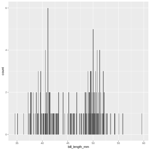
Now we only plot data from the male penguins, if we are particularly interested in those. This can be quite convenient if you have particularly large data and need to reduce it to get a proper idea of what the variables really look like.
Challenge 1
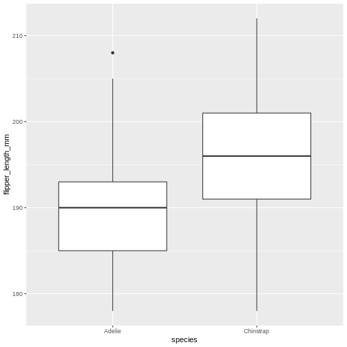
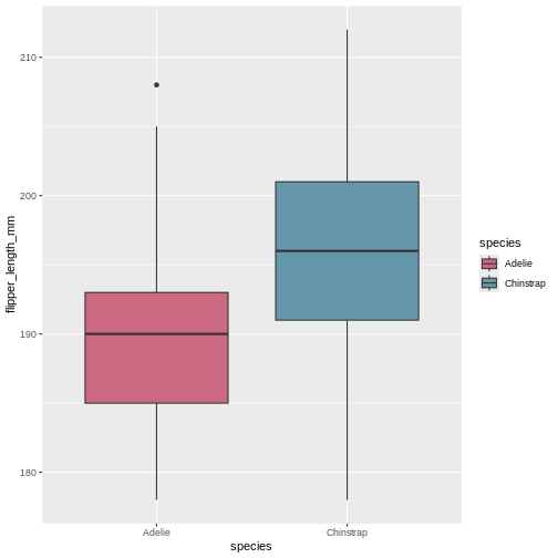
Create a plot of only data from the Dream island, putting flipper length on the y-axis and species on the x-axis. Make it a box-plot.
Try geom_boxplot
R
penguins |>
  filter(island == "Dream") |>
  ggplot(aes(x = species, y = flipper_length_mm)) +
  geom_boxplot()
Adding colour
This plot is a little boring, so let us spruce it up! How about
adding colour to the boxplot? We do this by using the
colour/color argument in ggplot2.
R
penguins |>
  filter(island == "Dream") |>
  ggplot(aes(x = species, y = flipper_length_mm)) +
  geom_boxplot(aes(colour = species))
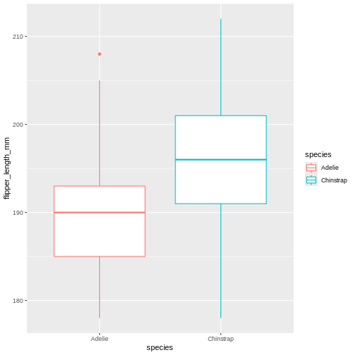
Did that look as you expected? Maybe you expected the rectangles of the boxes to be coloured, rather than the edges?
Challenge 2
Change the previous boxplot argument colour to
fill
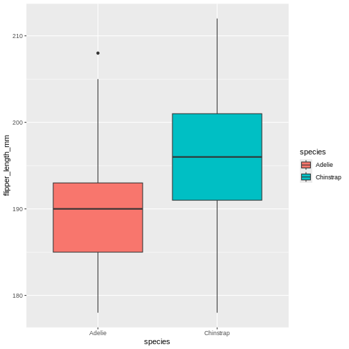
Learning the difference between using fill and
colour/color can take a little time, but in
general colour gives colour to edges, while fill floods elements.
R
penguins |>
  filter(island == "Dream") |>
  ggplot(aes(x = species, y = flipper_length_mm)) +
  geom_boxplot(aes(fill = species))
Changing colour
Now, default colours are well and fine for quick plots and exploring
data, but we usually all end up changing the colours when we start
preparing for publication or reports. In ggplot, we change the colours
using the scale_functions. The scale functions actually
cover much more than just colour/fill. They can change the types of
points in point plots, different types of scales for the axes
(logarithmic, percent, currency), and lots more! We will focus on
colour/fill here, but once you start exploring these options, there are
almost no limits to what you can do!
Let’s say you are publishing in a journal with strict policy on black and white only. Its better to prepare you plot in back and white your self, rather than relying on conversion of colour to black and white, you might be surprised at how little distinction there are between colours when the actually colour is stripped.
Let us start with the plot we just made, and test what types of
options we get when starting to add scale_fill_ in the
script. We get lots of preview options, “brewer”, “continuous”,
“gradient”, too many options?
There’s one called scale_fill_grey() let us try that one
for convenience!
R
penguins |>
  filter(island == "Dream") |>
  ggplot(aes(x = species, y = flipper_length_mm)) +
  geom_boxplot(aes(fill = species)) +
  scale_fill_grey()
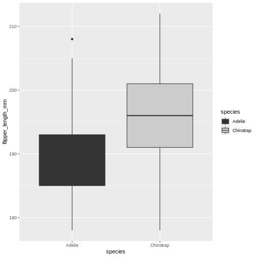
Ok! The colours are now changed, and the legend with it, quite convenient. But, the grey used is the same as for the lines, masking the median line for the Adelie box. That won’t do. Let us try something else.
R
penguins |>
  filter(island == "Dream") |>
  ggplot(aes(x = species, y = flipper_length_mm)) +
  geom_boxplot(aes(fill = species)) +
  scale_fill_manual(values = c("black", "white"))
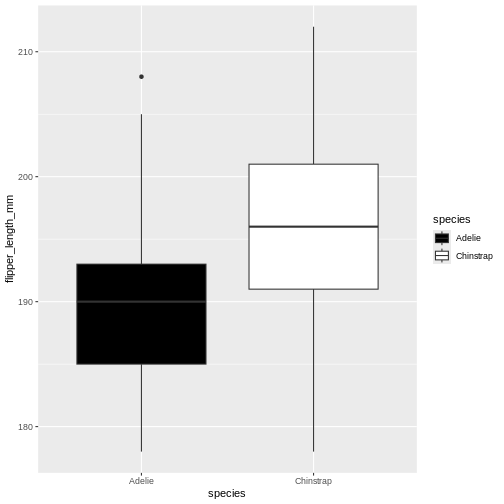
This is maybe a little stark, but the difference is clear between the
two, and that’s what we are after right now. Using the
manual version of scales means you manually add the colours
you want to use. You can specify colours by name and hexidecimal code,
whichever you find better to work with.
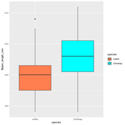
Challenge 3
Base you plot on the same as we have used so far. Change the colours to coral and cyan
“coral” and “cyan” are built in colour names, that you can call directly. There are lots of these names, datanovia has a great list of them
R
penguins |>
  filter(island == "Dream") |>
  ggplot(aes(x = species, y = flipper_length_mm)) +
  geom_boxplot(aes(fill = species)) +
  scale_fill_manual(values = c("coral", "cyan"))
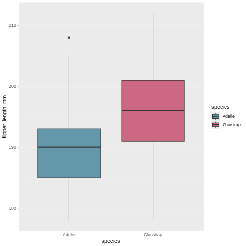
Challenge 4
Base you plot on the same as we have used so far. Change the colours to the hexidecmial colours “#6597aa” and “#cc6882”
hexidecimal colour codes are often use in webdesign, and are a way of coding red, blue and green. To explore colours in hexidecmial, there are lots of we resources like color-hex.com
R
penguins |>
  filter(island == "Dream") |>
  ggplot(aes(x = species, y = flipper_length_mm)) +
  geom_boxplot(aes(fill = species)) +
  scale_fill_manual(values = c("#6597aa", "#cc6882"))
Challenge 5
Base you plot on the same as we have used so far. Change the order for the hexidecimal colours in the previous plot. what did that do?
The order you provide the manual colours dictate which category gets which colour.
R
penguins |>
  filter(island == "Dream") |>
  ggplot(aes(x = species, y = flipper_length_mm)) +
  geom_boxplot(aes(fill = species)) +
  scale_fill_manual(values = c("#cc6882", "#6597aa"))
Challenge 6
Now, make an entirely different plot. Take the entire penguins dataset, and plot bill depth on the x-axis and bill length on the y. Create a point plot, with the points coloured by bill length. Try changing the colour of the points. What types of scales can you use?
There is not single answer here, there are many different options. The key difference between what we did before and this, is that the colouring scale is continuous, rather than categorical, so we need slightly different versions.
R
penguins |>
  ggplot(aes(x = bill_depth_mm, y = bill_length_mm)) +
  geom_point(aes(colour = bill_length_mm)) +
  scale_colour_viridis_c()
WARNING
Warning: Removed 2 rows containing missing values or values outside the scale range
(`geom_point()`).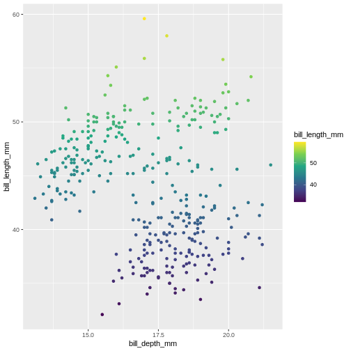
R
penguins |>
  ggplot(aes(x = bill_depth_mm, y = bill_length_mm)) +
  geom_point(aes(colour = bill_length_mm)) +
  scale_colour_gradientn(colours = c("#6597aa", "#cc6882"))
WARNING
Warning: Removed 2 rows containing missing values or values outside the scale range
(`geom_point()`).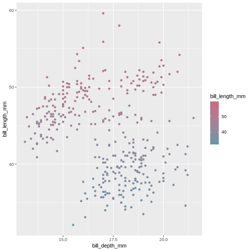
Changing the overall look
Now that we know more about changing the colours, we might want something else than the default look with the grey background etc. Just like with the default colours, it serves its generally quick look purpose, but we likely want to change it.
The theme() functions are there to help you get control
over how a plot looks. There are lots of different themes to choose
from, that form a great basis for all you need.
R
penguins |>
  ggplot(aes(x = bill_depth_mm, y = bill_length_mm)) +
  geom_point(aes(colour = bill_length_mm)) +
  scale_colour_gradientn(colours = c("#6597aa", "#cc6882")) +
  theme_minimal()
WARNING
Warning: Removed 2 rows containing missing values or values outside the scale range
(`geom_point()`).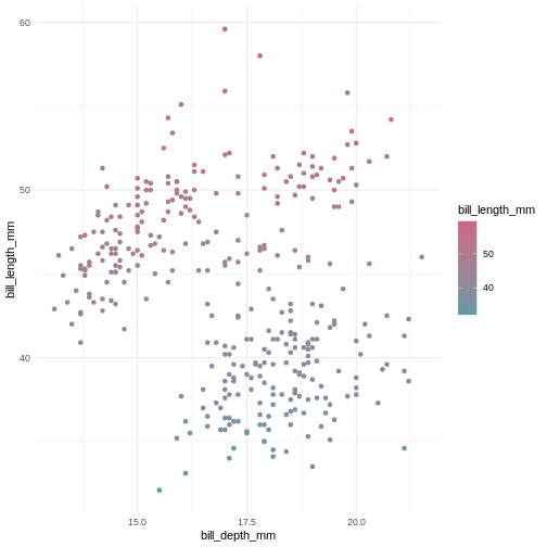
Here we have chosen theme_minimal() which strips axis
lines and the grey background, its more minimal. Explore some different
options by typing theme_ and pressing the tab
key to see what options there are.
Challenge 7
Use the same plot we have been working on, and change the theme to the “classic theme
The classic theme is one often wanted by strict and old-school journals. Its very handy to have a short-cut to it.
R
penguins |>
  ggplot(aes(x = bill_depth_mm, y = bill_length_mm)) +
  geom_point(aes(colour = bill_length_mm)) +
  scale_colour_gradientn(colours = c("#6597aa", "#cc6882")) +
  theme_classic()
WARNING
Warning: Removed 2 rows containing missing values or values outside the scale range
(`geom_point()`).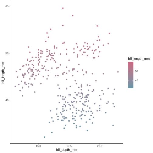
Challenge 8
Now try the void theme. Is this a meaningful theme to use for data plots=
The void theme strips all axis and background, leaving the plot alone. This is generally not a meaningful theme to use for publication, but could be good to use if you ever dwelve into the world of generative art.
R
penguins |>
  ggplot(aes(x = bill_depth_mm, y = bill_length_mm)) +
  geom_point(aes(colour = bill_length_mm)) +
  scale_colour_gradientn(colours = c("#6597aa", "#cc6882")) +
  theme_void()
WARNING
Warning: Removed 2 rows containing missing values or values outside the scale range
(`geom_point()`).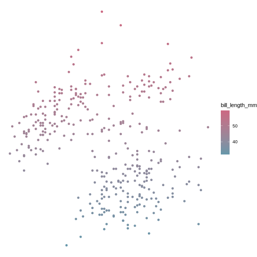
Wrap up
There is a lot more we could teach you about customising your plots to look how you want. There are many web resources you can look at to help you along they way, like on The MockUp. But if you dont want to deal with too many details, you can always isntall and use tne ggthemes package, which can create plots that look like your old favourite tools made them (like SPSS, Stata, excel. etc.).