Data manipulation with dplyr
Last updated on 2022-08-02 | Edit this page
Overview
Questions
- How can I add variables to my data?
- How can I alter the variables already in my data?
Objectives
- Use
mutate()to add and alter variables - Use
if_else()where appropriate - Use
case_when()where appropriate - Understand basic consents of different data types
Motivation
Often, the data we have do not contain exactly what we need. We might need to change the order of factors, create new variables based on other columns in the data, or even variables conditional on specific values in other columns.
Adding new variables,
In {tidyverse}, when we add new variables, we use the mutate() function. Just like the other {tidyverse} functions, mutate work specifically with data sets, and provides a nice shorthand for working directly with the columns in the data set.
R
penguins |>
  mutate(new_var = 1)
OUTPUT
# A tibble: 344 × 9
species island bill_length_mm bill_d…¹ flipp…² body_…³ sex year new_var
<fct> <fct> <dbl> <dbl> <int> <int> <fct> <int> <dbl>
1 Adelie Torgersen 39.1 18.7 181 3750 male 2007 1
2 Adelie Torgersen 39.5 17.4 186 3800 fema… 2007 1
3 Adelie Torgersen 40.3 18 195 3250 fema… 2007 1
4 Adelie Torgersen NA NA NA NA <NA> 2007 1
5 Adelie Torgersen 36.7 19.3 193 3450 fema… 2007 1
6 Adelie Torgersen 39.3 20.6 190 3650 male 2007 1
7 Adelie Torgersen 38.9 17.8 181 3625 fema… 2007 1
8 Adelie Torgersen 39.2 19.6 195 4675 male 2007 1
9 Adelie Torgersen 34.1 18.1 193 3475 <NA> 2007 1
10 Adelie Torgersen 42 20.2 190 4250 <NA> 2007 1
# … with 334 more rows, and abbreviated variable names ¹bill_depth_mm,
# ²flipper_length_mm, ³body_mass_g
# ℹ Use `print(n = ...)` to see more rowsThe output of this can be hard to spot, depending on the size of the screen. Let us for convenience create a subsetted data set to work on so we can easily see what we are doing.
R
penguins_s <- penguins |>
  select(1:3, starts_with("bill"))
Lets try our command again on this new data.
R
penguins_s |>
  mutate(new_var = 1)
OUTPUT
# A tibble: 344 × 5
   species island    bill_length_mm bill_depth_mm new_var
   <fct>   <fct>              <dbl>         <dbl>   <dbl>
 1 Adelie  Torgersen           39.1          18.7       1
 2 Adelie  Torgersen           39.5          17.4       1
 3 Adelie  Torgersen           40.3          18         1
 4 Adelie  Torgersen           NA            NA         1
 5 Adelie  Torgersen           36.7          19.3       1
 6 Adelie  Torgersen           39.3          20.6       1
 7 Adelie  Torgersen           38.9          17.8       1
 8 Adelie  Torgersen           39.2          19.6       1
 9 Adelie  Torgersen           34.1          18.1       1
10 Adelie  Torgersen           42            20.2       1
# … with 334 more rows
# ℹ Use `print(n = ...)` to see more rows
There is now a new column in the data set called “new_var”, and it has the value 1 for all rows! This is what we told mutate() to do! We specified a new column by name, and gave it a specific value, 1.
This works because its easy to assigning a single value to all rows. What if we try to give it three values? What would we expect?
R
penguins_s |>
  mutate(var = 1:3)
ERROR
Error in `mutate()`:
! Problem while computing `var = 1:3`.
✖ `var` must be size 344 or 1, not 3.
Here, it’s failing with a mysterious message. The error is telling us that input must be of size 344 or 1. 344 are the number of rows in the data set, so its telling us the input we gave it is not suitable because its neither of length 344 nor of length 1.
So now we know the premises for mutate, it takes inputs that are either of the same length as there are rows in the data set or length 1.
R
penguins_s |>
  mutate(var = 1:344)
OUTPUT
# A tibble: 344 × 5
   species island    bill_length_mm bill_depth_mm   var
   <fct>   <fct>              <dbl>         <dbl> <int>
 1 Adelie  Torgersen           39.1          18.7     1
 2 Adelie  Torgersen           39.5          17.4     2
 3 Adelie  Torgersen           40.3          18       3
 4 Adelie  Torgersen           NA            NA       4
 5 Adelie  Torgersen           36.7          19.3     5
 6 Adelie  Torgersen           39.3          20.6     6
 7 Adelie  Torgersen           38.9          17.8     7
 8 Adelie  Torgersen           39.2          19.6     8
 9 Adelie  Torgersen           34.1          18.1     9
10 Adelie  Torgersen           42            20.2    10
# … with 334 more rows
# ℹ Use `print(n = ...)` to see more rows
But generally, we create new columns based on other data in the data set. So let’s do a more useful example. For instance, perhaps we want to use the ratio between the bill length and depth as a measurement for a model.
R
penguins_s |>
  mutate(bill_ratio = bill_length_mm / bill_depth_mm)
OUTPUT
# A tibble: 344 × 5
   species island    bill_length_mm bill_depth_mm bill_ratio
   <fct>   <fct>              <dbl>         <dbl>      <dbl>
 1 Adelie  Torgersen           39.1          18.7       2.09
 2 Adelie  Torgersen           39.5          17.4       2.27
 3 Adelie  Torgersen           40.3          18         2.24
 4 Adelie  Torgersen           NA            NA        NA
 5 Adelie  Torgersen           36.7          19.3       1.90
 6 Adelie  Torgersen           39.3          20.6       1.91
 7 Adelie  Torgersen           38.9          17.8       2.19
 8 Adelie  Torgersen           39.2          19.6       2
 9 Adelie  Torgersen           34.1          18.1       1.88
10 Adelie  Torgersen           42            20.2       2.08
# … with 334 more rows
# ℹ Use `print(n = ...)` to see more rows
So, here we have asked for the ratio between bill length and depth to be calculated and stored in a column named bill_ratio. Then we selected just the bill columns to have a peak at the output more directly.
We can do almost anything within a mutate() to get the values as we want them, also use functions that exist in R to transform the data. For instance, perhaps we want to scale the variables of interest to have a mean of 0 and standard deviation of 1, which is quite common to improve statistical modelling. We can do that with the scale() function.
R
penguins_s |>
  mutate(bill_ratio = bill_length_mm / bill_depth_mm,
         bill_length_mm_z = scale(bill_length_mm))
OUTPUT
# A tibble: 344 × 6
species island bill_length_mm bill_depth_mm bill_ratio bill_length_mm_z[…¹
<fct> <fct> <dbl> <dbl> <dbl> <dbl>
1 Adelie Torgersen 39.1 18.7 2.09 -0.883
2 Adelie Torgersen 39.5 17.4 2.27 -0.810
3 Adelie Torgersen 40.3 18 2.24 -0.663
4 Adelie Torgersen NA NA NA NA
5 Adelie Torgersen 36.7 19.3 1.90 -1.32
6 Adelie Torgersen 39.3 20.6 1.91 -0.847
7 Adelie Torgersen 38.9 17.8 2.19 -0.920
8 Adelie Torgersen 39.2 19.6 2 -0.865
9 Adelie Torgersen 34.1 18.1 1.88 -1.80
10 Adelie Torgersen 42 20.2 2.08 -0.352
# … with 334 more rows, and abbreviated variable name ¹bill_length_mm_z[,1]
# ℹ Use `print(n = ...)` to see more rowsR
penguins_s |>
  mutate(bill_length_cm = bill_length_mm / 10)
OUTPUT
# A tibble: 344 × 5
   species island    bill_length_mm bill_depth_mm bill_length_cm
   <fct>   <fct>              <dbl>         <dbl>          <dbl>
 1 Adelie  Torgersen           39.1          18.7           3.91
 2 Adelie  Torgersen           39.5          17.4           3.95
 3 Adelie  Torgersen           40.3          18             4.03
 4 Adelie  Torgersen           NA            NA            NA
 5 Adelie  Torgersen           36.7          19.3           3.67
 6 Adelie  Torgersen           39.3          20.6           3.93
 7 Adelie  Torgersen           38.9          17.8           3.89
 8 Adelie  Torgersen           39.2          19.6           3.92
 9 Adelie  Torgersen           34.1          18.1           3.41
10 Adelie  Torgersen           42            20.2           4.2
# … with 334 more rows
# ℹ Use `print(n = ...)` to see more rowsR
penguins |>
  mutate(body_mass_kg = body_mass_g / 1000)
OUTPUT
# A tibble: 344 × 9
species island bill_length_mm bill_d…¹ flipp…² body_…³ sex year body_…⁴
<fct> <fct> <dbl> <dbl> <int> <int> <fct> <int> <dbl>
1 Adelie Torgersen 39.1 18.7 181 3750 male 2007 3.75
2 Adelie Torgersen 39.5 17.4 186 3800 fema… 2007 3.8
3 Adelie Torgersen 40.3 18 195 3250 fema… 2007 3.25
4 Adelie Torgersen NA NA NA NA <NA> 2007 NA
5 Adelie Torgersen 36.7 19.3 193 3450 fema… 2007 3.45
6 Adelie Torgersen 39.3 20.6 190 3650 male 2007 3.65
7 Adelie Torgersen 38.9 17.8 181 3625 fema… 2007 3.62
8 Adelie Torgersen 39.2 19.6 195 4675 male 2007 4.68
9 Adelie Torgersen 34.1 18.1 193 3475 <NA> 2007 3.48
10 Adelie Torgersen 42 20.2 190 4250 <NA> 2007 4.25
# … with 334 more rows, and abbreviated variable names ¹bill_depth_mm,
# ²flipper_length_mm, ³body_mass_g, ⁴body_mass_kg
# ℹ Use `print(n = ...)` to see more rowsAdding conditional variables
Sometimes, we want to assign certain data values based on other variables in the data set. For instance, maybe we want to classify all penguins with body mass above 4.5 kg as “large” while the rest are “normal”?
The if_else() function takes expressions, much like filter(). The first value after the expression is the value assigned if the expression is TRUE, while the second is if the expression is FALSE
R
penguin_weight <- penguins |>
  select(year, body_mass_g)

penguin_weight |>
  mutate(size = if_else(condition = body_mass_g > 4500,
                        true = "large",
                        false = "normal"))
OUTPUT
# A tibble: 344 × 3
    year body_mass_g size
   <int>       <int> <chr>
 1  2007        3750 normal
 2  2007        3800 normal
 3  2007        3250 normal
 4  2007          NA <NA>
 5  2007        3450 normal
 6  2007        3650 normal
 7  2007        3625 normal
 8  2007        4675 large
 9  2007        3475 normal
10  2007        4250 normal
# … with 334 more rows
# ℹ Use `print(n = ...)` to see more rows
Now we have a column with two values, large and normal based on whether the penguins are above or below 4.5 kilos.
We can for instance use that in a plot.
R
penguin_weight |>
  mutate(size = if_else(condition = body_mass_g > 4500,
                        true = "large",
                        false = "normal")) |>
  ggplot() +
  geom_jitter(mapping = aes(x = year, y = body_mass_g, colour = size))
WARNING
Warning: Removed 2 rows containing missing values (geom_point).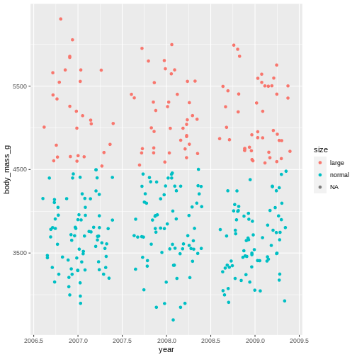
That shows us clearly that we have grouped the penguins based on their size. But there is this strange NA in the plot legend. what is that?
In R, missing values are usually given the value NA which stands for Not applicable, i.e., missing data. This is a very special name in R. Like TRUE and FALSE are capitalized, RStudio immediately recognizes the combination of capital letters and gives it another colour than all other values. In this case it means, there are some penguins we do not have the body mass of.
Now we know how to create new variables, and even how to make them if there are conditions on how to add the data.
But, we often want to add several columns of different types, and maybe even add new variables based on other new columns! Oh, it’s starting to sound complicated, but it does not have to be!
mutate() is so-called lazy-evaluated. This sounds weird, but it means that each new column you make is made in the sequence you make them. So as long as you think about the order of your mutate() creations, you can do that in a single mutate call.
R
penguins_s |>
  mutate(
    bill_ratio = bill_depth_mm / bill_length_mm,
    bill_type = if_else(condition = bill_ratio < 0.5,
                        true = "elongated",
                        false = "stumped")
  )
OUTPUT
# A tibble: 344 × 6
   species island    bill_length_mm bill_depth_mm bill_ratio bill_type
   <fct>   <fct>              <dbl>         <dbl>      <dbl> <chr>
 1 Adelie  Torgersen           39.1          18.7      0.478 elongated
 2 Adelie  Torgersen           39.5          17.4      0.441 elongated
 3 Adelie  Torgersen           40.3          18        0.447 elongated
 4 Adelie  Torgersen           NA            NA       NA     <NA>
 5 Adelie  Torgersen           36.7          19.3      0.526 stumped
 6 Adelie  Torgersen           39.3          20.6      0.524 stumped
 7 Adelie  Torgersen           38.9          17.8      0.458 elongated
 8 Adelie  Torgersen           39.2          19.6      0.5   stumped
 9 Adelie  Torgersen           34.1          18.1      0.531 stumped
10 Adelie  Torgersen           42            20.2      0.481 elongated
# … with 334 more rows
# ℹ Use `print(n = ...)` to see more rows
Now you’ve created two variables. One for bill_ratio, and then another one conditional on the values of the bill_ratio.
If you switched the order of these two, R would produce an error, because there would be no bill ratio to create the other column.
R
penguins_s |>
  mutate(
    bill_ratio = bill_depth_mm / bill_length_mm,
    bill_type = if_else(condition = bill_ratio < 0.5,
                        true = "elongated",
                        false = "stumped"),
    bill_ratio = bill_depth_mm / bill_length_mm
  )
OUTPUT
# A tibble: 344 × 6
   species island    bill_length_mm bill_depth_mm bill_ratio bill_type
   <fct>   <fct>              <dbl>         <dbl>      <dbl> <chr>
 1 Adelie  Torgersen           39.1          18.7      0.478 elongated
 2 Adelie  Torgersen           39.5          17.4      0.441 elongated
 3 Adelie  Torgersen           40.3          18        0.447 elongated
 4 Adelie  Torgersen           NA            NA       NA     <NA>
 5 Adelie  Torgersen           36.7          19.3      0.526 stumped
 6 Adelie  Torgersen           39.3          20.6      0.524 stumped
 7 Adelie  Torgersen           38.9          17.8      0.458 elongated
 8 Adelie  Torgersen           39.2          19.6      0.5   stumped
 9 Adelie  Torgersen           34.1          18.1      0.531 stumped
10 Adelie  Torgersen           42            20.2      0.481 elongated
# … with 334 more rows
# ℹ Use `print(n = ...)` to see more rows
But what if we want to categorize based on more than one condition? Nested if_else()?
R
penguins_s |>
  mutate(
    bill_ratio = bill_depth_mm / bill_length_mm,
    bill_type = if_else(condition = bill_ratio < 0.35,
                        true =  "elongated",
                        false = if_else(condition = bill_ratio < 0.45,
                                        true = "normal",
                                        false = "stumped")))
OUTPUT
# A tibble: 344 × 6
   species island    bill_length_mm bill_depth_mm bill_ratio bill_type
   <fct>   <fct>              <dbl>         <dbl>      <dbl> <chr>
 1 Adelie  Torgersen           39.1          18.7      0.478 stumped
 2 Adelie  Torgersen           39.5          17.4      0.441 normal
 3 Adelie  Torgersen           40.3          18        0.447 normal
 4 Adelie  Torgersen           NA            NA       NA     <NA>
 5 Adelie  Torgersen           36.7          19.3      0.526 stumped
 6 Adelie  Torgersen           39.3          20.6      0.524 stumped
 7 Adelie  Torgersen           38.9          17.8      0.458 stumped
 8 Adelie  Torgersen           39.2          19.6      0.5   stumped
 9 Adelie  Torgersen           34.1          18.1      0.531 stumped
10 Adelie  Torgersen           42            20.2      0.481 stumped
# … with 334 more rows
# ℹ Use `print(n = ...)` to see more rows
what if you have even more conditionals? It can get pretty messy pretty fast. Thankfully, {dplyr} has a smarter way of doing this, called case_when(). This function is similar to if_else(), but where you specify what each condition should be assigned. On the left you have the logical expression, and the on the right of the tilde (~) is the value to be assigned if that expression is TRUE
R
penguins_s |>
  mutate(
    bill_ratio = bill_depth_mm / bill_length_mm,
    bill_type = case_when(
      bill_ratio < 0.35 ~ "elongated",
      bill_ratio < 0.45 ~ "normal",
      TRUE              ~ "stumped")
  ) |>
  ggplot(mapping = aes(x = bill_length_mm,
                       y = bill_depth_mm,
                       colour = bill_type)) +
  geom_point()
WARNING
Warning: Removed 2 rows containing missing values (geom_point).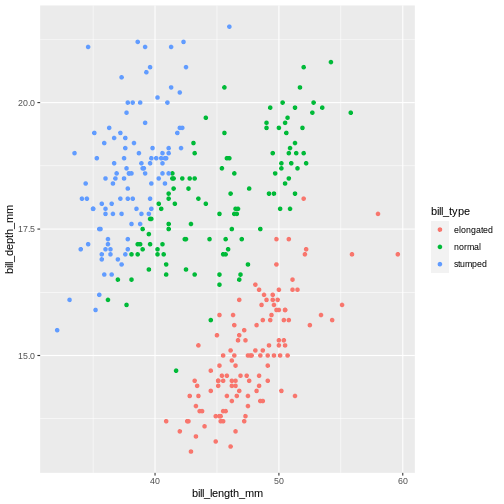
That looks almost the same. The NA’s are gone! That’s not right. We cannot categorize values that are missing. It’s our last statement that does this, which just says “make the remainder this value”. Which is not what we want. We need the NAs to stay NA’s.
case_when(), like the mutate(), evaluates the expressions in sequence. Which is why we can have two statements evaluating the same column with similar expressions (below 0.35 and then below 0.45). All values that are below 0.45 are also below 0.35. Since we first assign everything below 0.35, and then below 0.45, they do not collide. We can do the same for our last statement, saying that all values that are not NA should be given this category.
R
penguins |>
  mutate(
    bill_ratio = bill_depth_mm / bill_length_mm,
    bill_type = case_when(
      bill_ratio < 0.35  ~ "elongated",
      bill_ratio < 0.45  ~ "normal",
      !is.na(bill_ratio) ~ "stumped")
  ) |>
  ggplot(mapping = aes(x = bill_length_mm,
                       y = bill_depth_mm,
                       colour = bill_type)) +
  geom_point()
WARNING
Warning: Removed 2 rows containing missing values (geom_point).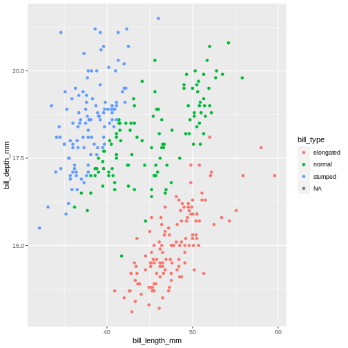
Here, we use the is.na(), which is a special function in R to detect NA values. But it also has an ! in front, what does that mean? In R’s logical expressions, the ! is a negation specifier. It means it flips the logical so the TRUE becomes FALSE, and vice versa. So here, it means the bill_ratio is not NA.
R
penguins |>
  mutate(bill_ld_ratio_log = log(bill_length_mm / bill_depth_mm))
OUTPUT
# A tibble: 344 × 9
species island bill_length_mm bill_d…¹ flipp…² body_…³ sex year bill_…⁴
<fct> <fct> <dbl> <dbl> <int> <int> <fct> <int> <dbl>
1 Adelie Torgersen 39.1 18.7 181 3750 male 2007 0.738
2 Adelie Torgersen 39.5 17.4 186 3800 fema… 2007 0.820
3 Adelie Torgersen 40.3 18 195 3250 fema… 2007 0.806
4 Adelie Torgersen NA NA NA NA <NA> 2007 NA
5 Adelie Torgersen 36.7 19.3 193 3450 fema… 2007 0.643
6 Adelie Torgersen 39.3 20.6 190 3650 male 2007 0.646
7 Adelie Torgersen 38.9 17.8 181 3625 fema… 2007 0.782
8 Adelie Torgersen 39.2 19.6 195 4675 male 2007 0.693
9 Adelie Torgersen 34.1 18.1 193 3475 <NA> 2007 0.633
10 Adelie Torgersen 42 20.2 190 4250 <NA> 2007 0.732
# … with 334 more rows, and abbreviated variable names ¹bill_depth_mm,
# ²flipper_length_mm, ³body_mass_g, ⁴bill_ld_ratio_log
# ℹ Use `print(n = ...)` to see more rowsChallenge 4
Create a new column called body_type, where animals below 3 kg are small, animals between 3 and 4.5 kg are normal, and animals larger than 4.5 kg are large. In the same command, create a new column named biscoe and its content should be TRUE if the island is Biscoe and FALSE for everything else.
R
penguins |>
  mutate(
    body_type = case_when(
       body_mass_g < 3000 ~ "small",
       body_mass_g >= 3000 & body_mass_g < 4500 ~ "normal",
       body_mass_g >= 4500 ~ "large"),
    biscoe = if_else(island == "Biscoe",
                     true = TRUE,
                     false = FALSE)
  )
OUTPUT
# A tibble: 344 × 10
species island bill_l…¹ bill_…² flipp…³ body_…⁴ sex year body_…⁵ biscoe
<fct> <fct> <dbl> <dbl> <int> <int> <fct> <int> <chr> <lgl>
1 Adelie Torgersen 39.1 18.7 181 3750 male 2007 normal FALSE
2 Adelie Torgersen 39.5 17.4 186 3800 fema… 2007 normal FALSE
3 Adelie Torgersen 40.3 18 195 3250 fema… 2007 normal FALSE
4 Adelie Torgersen NA NA NA NA <NA> 2007 <NA> FALSE
5 Adelie Torgersen 36.7 19.3 193 3450 fema… 2007 normal FALSE
6 Adelie Torgersen 39.3 20.6 190 3650 male 2007 normal FALSE
7 Adelie Torgersen 38.9 17.8 181 3625 fema… 2007 normal FALSE
8 Adelie Torgersen 39.2 19.6 195 4675 male 2007 large FALSE
9 Adelie Torgersen 34.1 18.1 193 3475 <NA> 2007 normal FALSE
10 Adelie Torgersen 42 20.2 190 4250 <NA> 2007 normal FALSE
# … with 334 more rows, and abbreviated variable names ¹bill_length_mm,
# ²bill_depth_mm, ³flipper_length_mm, ⁴body_mass_g, ⁵body_type
# ℹ Use `print(n = ...)` to see more rows