Autoregressive Forecasts
Last updated on 2023-08-20 | Edit this page
Overview
Questions
- How can we enhance our models to account for autoregression?
Objectives
- Explain the parameters of order argument of the
statsmodelsSARIMAX model. - Refine forecasts to account for autoregressive processes.
Introduction
In this section we will continue to use the same subset of data to refine our time-series forecasts. We have seen how we can improve forecasts by differencing data so that time-series are stationary.
However, as noted in our earlier results our forecasts are still not as accurate as we’d like them to be. This is because in addition to not being stationary, our data include autoregressive processes. That is, values for power consumption can be affected by previous values of the same variable.
About the code
The code used in this lesson is based on and, in some cases, a direct application of code used in the Manning Publications title, Time series forecasting in Python, by Marco Peixeiro.
Peixeiro, Marco. Time Series Forecasting in Python. [First edition]. Manning Publications Co., 2022.
The original code from the book is made available under an Apache 2.0 license. Use and application of the code in these materials is within the license terms, although this lesson itself is licensed under a Creative Commons CC-BY 4.0 license. Any further use or adaptation of these materials should cite the source code developed by Peixeiro:
Peixeiro, Marco. Timeseries Forecasting in Python [Software code]. 2022. Accessed from https://github.com/marcopeix/TimeSeriesForecastingInPython.
Create data subset
Since we have been using the same process to read and subset a single data file, this time we will write a function that includes the necessary commands. This will make our process more flexible in case we want to change the date range or the resampling frequency and test our models on different subsets.
First we need to import the same libraries as before.
PYTHON
import pandas as pd
import numpy as np
import matplotlib.pyplot as plt
from statsmodels.tsa.stattools import adfuller
from statsmodels.graphics.tsaplots import plot_acf
from statsmodels.graphics.tsaplots import plot_pacf
from statsmodels.tsa.statespace.sarimax import SARIMAX
from sklearn.metrics import mean_squared_error
from sklearn.metrics import mean_absolute_error
Now, define a function that takes the name of a data file, a start and end date for a date range, and a resampling frequency as arguments.
PYTHON
def subset_resample(fpath, sample_freq, start_date, end_date=None):
    df = pd.read_csv(fpath)
    df.set_index(pd.to_datetime(df["INTERVAL_TIME"]), inplace=True)
    df.sort_index(inplace=True)
    if end_date:
        date_subset = df.loc[start_date: end_date].copy()
    else:
        date_subset = df.loc[start_date].copy()
    resampled_data = date_subset.resample(sample_freq)
    return resampled_data
Note that the returned object is not a data frame - it’s a DatetimeIndexResampler, which is a kind of group in Pandas.
PYTHON
fp = "../../data/ladpu_smart_meter_data_01.csv"
data_subset_resampled = subset_resample(fp, "D", "2019-01", end_date="2019-07")
print("Data type of returned object:", type(data_subset_resampled))
We can create a dataframe for forecasting by aggregating the data using a specific metric. In this case, we will use the sum of the daily “INTERVAL_READ” values.
PYTHON
daily_usage = data_subset_resampled['INTERVAL_READ'].agg([np.sum])
print(daily_usage.info())
print(daily_usage.head())
OUTPUT
<class 'pandas.core.frame.DataFrame'>
DatetimeIndex: 212 entries, 2019-01-01 to 2019-07-31
Freq: D
Data columns (total 1 columns):
 #   Column  Non-Null Count  Dtype
---  ------  --------------  -----
 0   sum     212 non-null    float64
dtypes: float64(1)
memory usage: 3.3 KB
None
                   sum
INTERVAL_TIME
2019-01-01      7.5324
2019-01-02     10.2534
2019-01-03      6.8544
2019-01-04      5.3250
2019-01-05      7.5480
We can further inspect the data by plotting.
PYTHON
fig, ax = plt.subplots()

ax.plot(daily_usage['sum'])
ax.set_xlabel('Time')
ax.set_ylabel('Daily electricity consumption')

fig.autofmt_xdate()
plt.tight_layout()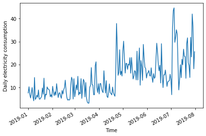
Determine order of autoregressive process
As before, we will also calculate the AD Fuller statistic on the data.
PYTHON
adfuller_test = adfuller(daily_usage)
print(f'ADFuller result: {adfuller_test[0]}')
print(f'p-value: {adfuller_test[1]}')
OUTPUT
ADFuller result: -2.533089941397639
p-value: 0.10762933815081588
The result indicates that the data are not stationary, so we will difference the data and recalculate the AD Fuller statistic.
PYTHON
daily_usage_diff = np.diff(daily_usage['sum'], n = 1)
adfuller_test = adfuller(daily_usage_diff)
print(f'ADFuller result: {adfuller_test[0]}')
print(f'p-value: {adfuller_test[1]}')
OUTPUT
ADFuller result: -7.966077912452976
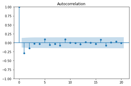
p-value: 2.8626643210939594e-12Plotting the autocorrelation function suggests an autoregressive process occurring within the data.
The order argument of the SARIMAX model that we are using for our forecasts includes a parameter for specifying the order of the autoregressive process. We can plot the partial autocorrelation function to determine this.
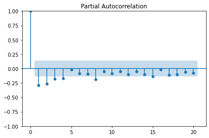
The plot indicates significant autoregression up to the fourth lag, so we have an autoregressive process of order 4, or AR(4).
Forecast an autoregressive process
With the order of the autoregressive process known, we can revise our
forecasting function to pass this new parameter to the SARIMAX model
from sklearn.
First, we will create training and test datasets and plot to show the range of values we will forecast.
PYTHON
df_diff = pd.DataFrame({'daily_usage': daily_usage_diff})

train = df_diff[:int(len(df_diff) * .9)] # ~90% of data
test = df_diff[int(len(df_diff) * .9):] # ~10% of data
print("Training data length:", len(train))
print("Test data length:", len(test))
OUTPUT
Training data length: 189
Test data length: 22
And the plot:
PYTHON
fig, (ax1, ax2) = plt.subplots(nrows=2, ncols=1, sharex=True,
                               figsize=(10, 8))

ax1.plot(daily_usage['sum'].values)
ax1.set_xlabel('Time')
ax1.set_ylabel('Energy use')
ax1.axvspan(190, 211, color='#808080', alpha=0.2)

ax2.plot(df_diff['daily_usage'])
ax2.set_xlabel('Time')
ax2.set_ylabel('Energy use - diff')
ax2.axvspan(190, 211, color='#808080', alpha=0.2)

fig.autofmt_xdate()
plt.tight_layout()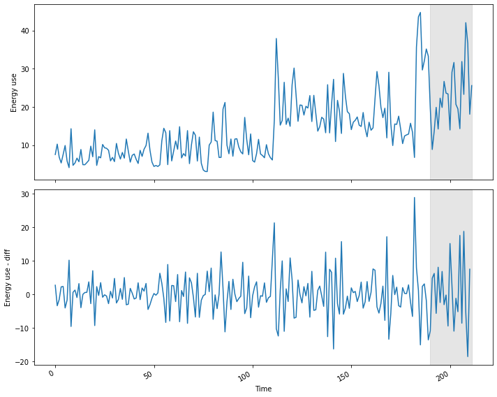
We are also going to update our function from the previous section,
in which we hard-coded a value for the order of the autoregressive
process in the order argument of the SARIMAX model. Here we
generalize the function name to model_forecast() and we are
now using arguments, ar_order and ma_order, to pass
two of the three parameters required by the order argument of
the model.
As before, we will use the last known value as our baseline metric for evaluating the performance of the updated model.
PYTHON
def last_known(data, training_len, horizon, window):
    total_len = training_len + horizon
    pred_last_known = []

    for i in range(training_len, total_len, window):
        subset = data[:i]
        last_known = subset.iloc[-1].values[0]
        pred_last_known.extend(last_known for v in range(window))

    return pred_last_known

def model_forecast(data, training_len, horizon, ar_order, ma_order, window):
    total_len = training_len + horizon
    model_predictions = []

    for i in range(training_len, total_len, window):
        model = SARIMAX(data[:i], order=(ar_order, 0, ma_order))
        res = model.fit(disp=False)
        predictions = res.get_prediction(0, i + window - 1)
        oos_pred = predictions.predicted_mean.iloc[-window:]
        model_predictions.extend(oos_pred)

    return model_predictions
Now we can call our functions to forecast power consumption. For comparison sake we will also make a prediction using the moving average forecast from the last section. Recall that the order of the moving average process was 2, and the order of the autoregressive process is 4.
PYTHON
TRAIN_LEN = len(train)
HORIZON = len(test)
WINDOW = 1

pred_last_value = last_known(df_diff, TRAIN_LEN, HORIZON, WINDOW)
pred_MA = model_forecast(df_diff, TRAIN_LEN, HORIZON, 0, 2, WINDOW)
pred_AR = model_forecast(df_diff, TRAIN_LEN, HORIZON, 4, 0, WINDOW)

test['pred_last_value'] = pred_last_value
test['pred_MA'] = pred_MA
test['pred_AR'] = pred_AR

print(test.head())
OUTPUT
     daily_usage  pred_last_value   pred_MA   pred_AR
189     -13.5792          -1.8630 -1.870535  1.735114
190     -10.8660         -13.5792  4.425102  5.553305
191       4.8054         -10.8660  9.760944  9.475778
192       6.2280           4.8054  7.080340  5.395541
193      -5.6718           6.2280  2.106354  0.205880
Plotting the result shows that the results of the moving average and autoregressive forecasts are very similar.
PYTHON
fig, ax = plt.subplots()

ax.plot(df_diff[150:]['daily_usage'], 'b-', label='actual')
ax.plot(test['pred_last_value'], 'r-.', label='last')
ax.plot(test['pred_MA'], 'g-.', label='MA(2)')
ax.plot(test['pred_AR'], 'k--', label='AR(4)')

ax.axvspan(190, 211, color='#808080', alpha=0.2)
ax.legend(loc=2)

ax.set_xlabel('Time')
ax.set_ylabel('Energy use - diff')

plt.tight_layout()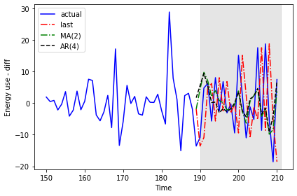
Calculating the mean squared error for each forecast indicates that of the three forecasting methods, the moving average performs the best.
PYTHON
mse_last = mean_squared_error(test['daily_usage'], test['pred_last_value'])
mse_MA = mean_squared_error(test['daily_usage'], test['pred_MA'])
mse_AR = mean_squared_error(test['daily_usage'], test['pred_AR'])

print("MSE of last known value forecast:", mse_last)
print("MSE of MA(2) forecast:",mse_MA)
print("MSE of AR(4) forecast:",mse_AR)
OUTPUT
MSE of last known value forecast: 252.6110739163637
MSE of MA(2) forecast: 73.404918547051
MSE of AR(4) forecast: 85.29189129936279
Given the choice between these three results, we would apply the moving average forecast to our data. For the purposes of demonstration, however, we will reverse transform our differenced data with the autoregressive forecast results.
PYTHON
daily_usage['pred_usage'] = pd.Series()
daily_usage['pred_usage'][190:] = daily_usage['sum'].iloc[190] + test['pred_AR'].cumsum()
print(daily_usage.tail())
OUTPUT
                   sum  pred_usage
INTERVAL_TIME
2019-07-27     23.2752   34.683237
2019-07-28     42.0504   33.145726
2019-07-29     36.6444   24.039123
2019-07-30     18.0828   19.823836
2019-07-31     25.5774   26.623576
Finally we can plot the transformed forecasts with the actual power consumption values for comparison, and perform a final evaluation using the mean absolute error. As expected from the results of the mean squared error calculated above, the mean absolute error for the autoregressive forecast will be higher than that reported for the moving average forecast in the previous section.
PYTHON
mae_MA_undiff = mean_absolute_error(daily_usage['sum'].iloc[191:],
                                    daily_usage['pred_usage'].iloc[191:])

print("Mean absolute error, AR(4):", mae_MA_undiff)
OUTPUT
Mean absolute error, AR(4): 13.074409772576958Plot code:
PYTHON
fig, ax = plt.subplots()

ax.plot(daily_usage['sum'].values, 'b-', label='actual')
ax.plot(daily_usage['pred_usage'].values, 'k--', label='AR(4)')

ax.legend(loc=2)

ax.set_xlabel('Time')
ax.set_ylabel('Energy consumption')
ax.axvspan(190, 211, color='#808080', alpha=0.2)
ax.set_xlim(170, 211)

fig.autofmt_xdate()
plt.tight_layout()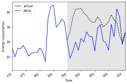
Key Points
- The order argument of the SARIMAX model includes parameters for the order of autoregressive and moving average processes.