All in One View
Content from Short Introduction to Programming in Python
Last updated on 2024-02-13 | Edit this page
Overview
Questions
- What is Python?
- Why should I learn Python?
Objectives
- Describe the advantages of using programming vs. completing repetitive tasks by hand.
- Define the following data types in Python: strings, integers, and floats.
- Perform mathematical operations in Python using basic operators.
- Define the following as it relates to Python: lists, tuples, and dictionaries.
The Basics of Python
Python is a general purpose programming language that supports rapid development of scripts and applications.
Python’s main advantages:
- Open Source software, supported by Python Software Foundation
- Available on all platforms
- It is a general-purpose programming language
- Supports multiple programming paradigms
- Very large community with a rich ecosystem of third-party packages
Interpreter
Python is an interpreted language which can be used in two ways:
- “Interactive” Mode: It functions like an “advanced calculator” Executing one command at a time:
PYTHON
user:host:~$ python
Python 3.5.1 (default, Oct 23 2015, 18:05:06)
[GCC 4.8.3] on linux2
Type "help", "copyright", "credits" or "license" for more information.
>>> 2 + 2
4
>>> print("Hello World")
Hello World- “Scripting” Mode: Executing a series of “commands” saved in text
file, usually with a
.pyextension after the name of your file:
Introduction to Python built-in data types
Strings, integers and floats
Python has built-in numeric types for integers, floats, and complex numbers. Strings are a built-in textual type.:
Here we’ve assigned data to variables, namely text,
number and pi_value, using the assignment
operator =. The variable called text is a
string which means it can contain letters and numbers. Notice that in
order to define a string you need to have quotes around your text. To
print out the value stored in a variable we can simply type the name of
the variable into the interpreter:
However, in a script, a print function is needed to
output the text:
example.py
PYTHON
# A Python script file
# Comments in Python start with #
# The next line uses the print function to print out the text string
print(text)
Running the script
Tip: The print function is a built-in
function in Python. Later in this lesson, we will introduce methods and
user-defined functions. The Python documentation is excellent for
reference on the differences between them.
Operators
We can perform mathematical calculations in Python using the basic
operators +, -, /, *, %:
PYTHON
>>> 2 + 2   #  addition
4
>>> 6 * 7   #  multiplication
42
>>> 2 ** 16  # power
65536
>>> 13 % 5  # modulo
3
We can also use comparison and logic operators:
<, >, ==, !=, <=, >= and statements of identity
such as and, or, not. The data type returned by this is
called a boolean.
Sequential types: Lists and Tuples
Lists
Lists are a common data structure to hold an ordered sequence of elements. Each element can be accessed by an index. Note that Python indexes start with 0 instead of 1:
A for loop can be used to access the elements in a list
or other Python data structure one at a time:
Indentation is very important in Python. Note that
the second line in the example above is indented. Just like three
chevrons >>> indicate an interactive prompt in
Python, the three dots ... are Python’s prompt for multiple
lines. This is Python’s way of marking a block of code. [Note: you do
not type >>> or ....]
To add elements to the end of a list, we can use the
append method. Methods are a way to interact with an object
(a list, for example). We can invoke a method using the dot
. followed by the method name and a list of arguments in
parentheses. Let’s look at an example using append:
To find out what methods are available for an object, we can use the
built-in help command:
Tuples
A tuple is similar to a list in that it’s an ordered sequence of
elements. However, tuples can not be changed once created (they are
“immutable”). Tuples are created by placing comma-separated values
inside parentheses ().
PYTHON
# tuples use parentheses
a_tuple= (1, 2, 3)
another_tuple = ('blue', 'green', 'red')
# Note: lists use square brackets
a_list = [1, 2, 3]Challenge - Tuples
- What happens when you type
a_tuple[2]=5vsa_list[1]=5? - Type
type(a_tuple)into python - what is the object type?
Dictionaries
A dictionary is a container that holds pairs of objects - keys and values.
Dictionaries work a lot like lists - except that you index them with keys. You can think about a key as a name for or a unique identifier for a set of values in the dictionary. Keys can only have particular types - they have to be “hashable”. Strings and numeric types are acceptable, but lists aren’t.
PYTHON
>>> rev = {1: 'one', 2: 'two'}
>>> rev[1]
'one'
>>> bad = {[1, 2, 3]: 3}
Traceback (most recent call last):
  File "<stdin>", line 1, in <module>
TypeError: unhashable type: 'list'
In Python, a “Traceback” is an multi-line error block printed out for the user.
To add an item to the dictionary we assign a value to a new key:
Using for loops with dictionaries is a little more
complicated. We can do this in two ways:
PYTHON
>>> for key, value in rev.items():
...     print(key, '->', value)
...
1 -> one
2 -> two
3 -> three
or
PYTHON
>>> for key in rev.keys():
...     print(key, '->', rev[key])
...
1 -> one
2 -> two
3 -> three
>>>Challenge - Can you do reassignment in a dictionary?
It is important to note that dictionaries are “unordered” and do not remember the sequence of their items (i.e. the order in which key:value pairs were added to the dictionary). Because of this, the order in which items are returned from loops over dictionaries might appear random and can even change with time.
Functions
Defining a section of code as a function in Python is done using the
def keyword. For example a function that takes two
arguments and returns their sum can be defined as:
Key points about functions are:
- definition starts with
def - function body is indented
-
returnkeyword precedes returned value
Content from Starting With Data
Last updated on 2024-02-13 | Edit this page
Overview
Questions
- How can I import data in Python?
- What is Pandas?
- Why should I use Pandas to work with data?
Objectives
- Navigate the workshop directory and download a dataset.
- Explain what a library is and what libraries are used for.
- Describe what the Python Data Analysis Library (Pandas) is.
- Load the Python Data Analysis Library (Pandas).
- Use
read_csvto read tabular data into Python. - Describe what a DataFrame is in Python.
- Access and summarize data stored in a DataFrame.
- Define indexing as it relates to data structures.
- Perform basic mathematical operations and summary statistics on data in a Pandas DataFrame.
- Create simple plots.
Working With Pandas DataFrames in Python
We can automate the processes listed above using Python. It is efficient to spend time building code to perform these tasks because once it is built, we can use our code over and over on different datasets that share a similar format. This makes our methods easily reproducible. We can also share our code with colleagues so they can replicate our analysis.
Starting in the same spot
To help the lesson run smoothly, let’s ensure everyone is in the same directory. This should help us avoid path and file name issues. At this time please navigate to the workshop directory. If you working in IPython Notebook be sure that you start your notebook in the workshop directory.
A quick aside that there are Python libraries like OS Library that can work with our directory structure, however, that is not our focus today.
Alex’s Processing
Alex is a researcher who is interested in Early English books. Alex knows the EEBO dataset and refers to it to find data such as titles, places, and authors. As well as searching for titles, they want to create some exploratory plots and intermediate datasets.
Alex can do some of this work using spreadsheet systems but this can be time consuming to do and revise. It can lead to mistakes that are hard to detect.
The next steps show how Python can be used to automate some of the processes.
As a result of creating Python scripts, the data can be re-run in the future.
Our Data
For this lesson, we will be using the EEBO catalogue data, a subset of the data from EEBO/TCP Early English Books Online/Text Creation Partnership
We will be using files from the data folder. This section will use
the eebo.csv file that can be found in your data
folder.
We are studying the authors and titles published marked up by the
Text Creation Partnership. The dataset is stored as a comma separated
(.csv) file, where each row holds information for a single
title, and the columns represent diferent aspects (variables) of each
entry:
| Column | Description |
|---|---|
| TCP | TCP identity |
| EEBO | EEBO identity |
| VID | VID identity |
| STC | STC identity |
| status | Whether the book is free or not |
| Author | Author(s) |
| Date | Date of publication |
| Title | The Book title |
| Terms | Terms associated with the text |
| Page Count | Number of pages in the text |
| Place | Location where the work was published |
If we open the eebo.csv data file using a text editor,
the first few rows of our first file look like this:
TCP,EEBO,VID,STC,Status,Author,Date,Title,Terms,Page Count,Place
A00002,99850634,15849,STC 1000.5; ESTC S115415,Free,"Aylett, Robert, 1583-1655?",1625,"The brides ornaments viz. fiue meditations, morall and diuine. 1. Knowledge, 2. zeale, 3. temperance, 4. bountie, 5. ioy.",,134,London
A00005,99842408,7058,STC 10000; ESTC S106695,Free,"Higden, Ranulf, d. 1364. Polycronicon. English. Selections.; Trevisa, John, d. 1402.",1515,Here begynneth a shorte and abreue table on the Cronycles ...; Saint Albans chronicle.,Great Britain -- History -- To 1485 -- Early works to 1800.; England -- Description and travel -- Early works to 1800.,302,London
A00007,99844302,9101,STC 10002; ESTC S108645,Free,"Higden, Ranulf, d. 1364. Polycronicon.",1528,"The Cronycles of Englonde with the dedes of popes and emperours, and also the descripcyon of Englonde; Saint Albans chronicle.",Great Britain -- History -- To 1485 -- Early works to 1800.; England -- Description and travel -- Early works to 1800.,386,London
A00008,99848896,14017,STC 10003; ESTC S113665,Free,"Wood, William, fl. 1623, attributed name.",1623,Considerations vpon the treaty of marriage between England and Spain,Great Britain -- Foreign relations -- Spain.,14,The Netherlands?
A00011,99837000,1304,STC 10008; ESTC S101178,Free,,1640,"Englands complaint to Iesus Christ, against the bishops canons of the late sinfull synod, a seditious conuenticle, a packe of hypocrites, a sworne confederacy, a traiterous conspiracy ... In this complaint are specified those impieties and insolencies, which are most notorious, scattered through the canons and constitutions of the said sinfull synod. And confuted by arguments annexed hereunto.",Church of England. -- Thirty-nine Articles -- Controversial literature.; Canon law -- Early works to 1800.,54,Amsterdam
A00012,99853871,19269,STC 1001; ESTC S118664,Free,"Aylett, Robert, 1583-1655?",1623,"Ioseph, or, Pharoah's fauourite; Joseph.",Joseph -- (Son of Jacob) -- Early works to 1800.,99,London
A00014,33143147,28259,STC 10011.6; ESTC S3200,Free,,1624,Greate Brittaines noble and worthy councell of warr,"England and Wales. -- Privy Council -- Portraits.; Great Britain -- History -- James I, 1603-1625.; Broadsides -- London (England) -- 17th century.",1,London
A00015,99837006,1310,STC 10011; ESTC S101184,Free,"Jones, William, of Usk.",1607,"Gods vvarning to his people of England By the great ouer-flowing of the vvaters or floudes lately hapned in South-wales and many other places. Wherein is described the great losses, and wonderfull damages, that hapned thereby: by the drowning of many townes and villages, to the vtter vndooing of many thousandes of people.",Floods -- Wales -- Early works to 1800.,16, London
A00018,99850740,15965,STC 10015; ESTC S115521,Free,,1558,The lame[n]tacion of England; Lamentacion of England.,"Great Britain -- History -- Mary I, 1553-1558 -- Early works to 1800.",26,Germany?
About Libraries
A library in Python contains a set of tools (functions) that perform different actions on our data. Importing a library is like getting a set of particular tools out of a storage locker and setting them up on the bench for use in a project. Once a library is set up, its functions can be used or called to perform different tasks.
Pandas in Python
One of the best options for working with tabular data in Python is to use the Python Data Analysis Library (a.k.a. Pandas Library). The Pandas library provides structures to sort our data, can produce high quality plots in conjunction with other libraries such as matplotlib, and integrates nicely with libraries that use NumPy (which is another common Python library) arrays.
Python doesn’t load all of the libraries available to it by default.
We have to add an import statement to our code in order to
use library functions required for our project. To import a library, we
use the syntax import libraryName, where
libraryName represents the name of the specific library we
want to use. Note that the import command calls a library
that has been installed previously in our system. If we use the
import command to call for a library that does not exist in
our local system, the command will throw and error when executed. In
this case, you can use pip command in another termina
window to install the missing libraries. See
here for details on how to do this.
Moreover, if we want to give the library a nickname to shorten the
command, we can add as nickNameHere. An example of
importing the pandas library using the common nickname pd
is:
Each time we call a function that’s in a library, we use the syntax
LibraryName.FunctionName. Adding the library name with a
. before the function name tells Python where to find the
function. In the example above, we have imported Pandas as
pd. This means we don’t have to type out
pandas each time we call a Pandas function.
Reading CSV Data Using Pandas
We will begin by locating and reading our survey data which are in
CSV format. We can use Pandas’ read_csv function to pull
either a local (a file in our machine) or a remote (one that is
available for downloading from the web) file into a Pandas table or DataFrame.
In order to read data in, we need to know where the data is stored on your computer or its URL address if the file is available on the web. It is recommended to place the data files in the same directory as the Jupyter notebook if working with local files
PYTHON
# note that pd.read_csv is used because we imported pandas as pd
# note that this assumes that the data file is in the same location
# as the Jupyter notebook
pd.read_csv("eebo.csv")
So What’s a DataFrame?
A DataFrame is a 2-dimensional data structure that can store data of
different types (including characters, integers, floating point values,
factors and more) in columns. It is similar to a spreadsheet or a
data.frame in R. A DataFrame always has an index (0-based).
An index refers to the position of an element in the data structure.
In a terminal window the above command yields the output below. However, the output may differ slightly if using Jupyter Notebooks:
          TCP        EEBO     VID  \
0      A00002  99850634.0   15849
1      A00005  99842408.0    7058
2      A00007  99844302.0    9101
3      A00008  99848896.0   14017
4      A00011  99837000.0    1304
...
146  A00525  99856552        ...                854   Prentyd  London
147  A00527  99849909        ...                 72            London
148  A00535  99849912        ...                106        Saint-Omer
[148 rows x 11 columns]
We can see that there were 149 rows parsed. Each row has 11 columns.
The first column displayed is the index of the
DataFrame. The index is used to identify the position of the data, but
it is not an actual column of the DataFrame. It looks like the
read_csv function in Pandas read our file properly.
However, we haven’t saved any data to memory so we can not work with it
yet. We need to assign the DataFrame to a variable so we can call and
use the data. Remember that a variable is a name given to a value, such
as x, or data. We can create a new object with
a variable name by assigning a value to it using =.
Let’s call the imported survey data eebo_df:
Notice that when you assign the imported DataFrame to a variable,
Python does not produce any output on the screen. We can print the value
of the eebo_df object by typing its name into the Python
command prompt.
which prints contents like above
Manipulating Our Index Data
Now we can start manipulating our data. First, let’s check the data
type of the data stored in eebo_df using the
type method. The type method and
__class__ attribute tell us that
eebo_df is
<class 'pandas.core.frame.DataFrame'>.
We can also enter eebo_df.dtypes at our prompt to view
the data type for each column in our DataFrame. int64
represents numeric integer values - int64 cells can not
store decimals. object represents strings (letters and
numbers). float64 represents numbers with decimals.
eebo_df.dtypeswhich returns:
TCP         object
EEBO        int64
VID         int64
STC         object
Status      object
Author      object
Date        int64
Title       object
Terms       object
Page Count  int64
Place       object
dtype: object
We’ll talk a bit more about what the different formats mean in a different lesson.
Useful Ways to View DataFrame objects in Python
We can use attributes and methods provided by the DataFrame object to summarize and access the data stored in it.
To access an attribute, use the DataFrame object name followed by the
attribute name df_object.attribute. For example, we can
access the Index
object containing the column names of eebo_df by using
its columns attribute
As we will see later, we can use the contents of the Index object to extract (slice) specific records from our DataFrame based on their values.
Methods are called by using the syntax
df_object.method(). Note the inclusion of open brackets at
the end of the method. Python treats methods as
functions associated with a dataframe rather than just
a property of the object as with attributes. Similarly to functions,
methods can include optional parameters inside the brackets to change
their default behaviour.
As an example, eebo_df.head() gets the first few rows in
the DataFrame eebo_df using the head()
method. With a method, we can supply extra information within
the open brackets to control its behaviour.
Let’s look at the data using these.
Challenge - DataFrames
Using our DataFrame eebo_df, try out the attributes
& methods below to see what they return.
eebo_df.columnseebo_df.shapeTake note of the output ofshape- what format does it return the shape of the DataFrame in?
HINT: More on tuples, here.
eebo_df.head()Also, what doeseebo_df.head(15)do?eebo_df.tail()
Calculating Statistics From Data In A Pandas DataFrame
We’ve read our data into Python. Next, let’s perform some quick summary statistics to learn more about the data that we’re working with. We might want to know how many different authors are included in our dataset, or how many works were published in a given year. We can perform summary stats quickly using groups. But first we need to figure out what we want to group by.
Let’s begin by exploring our data:
which returns:
array(['TCP', 'EEBO', 'VID', 'STC', 'Status', 'Author', 'Date', 'Title',
       'Terms', 'Page Count', 'Place'], dtype=object)
Let’s get a list of all the page counts. The pd.unique
function tells us all of the unique values in the Pages
column.
which returns:
PYTHON
array([134, 302, 386,  14,  54,  99,   1,  16,  26,  62,  50,  66,  30,
         6,  36,   8,  12,  24,  22,   7,  20,  40,  38,  13,  28,  10,
        23,   2, 112,  18,   4,  27,  42,  17,  46,  58, 200, 158,  65,
        96, 178,  52, 774,  81, 392,  74, 162,  56, 100, 172,  94,  79,
       107,  48, 102, 343, 136,  70, 156, 133, 228, 357, 110,  72,  44,
        43,  37,  98, 566, 500, 746, 884, 254, 618, 274, 188, 374,  47,
34, 177, 82, 78, 64, 124, 80, 108, 182, 120, 68, 854, 106])Challenge - Statistics
Create a list of unique locations found in the index data. Call it
places. How many unique location are there in the data?What is the difference between
len(places)andeebo_df['Place'].nunique()?
Groups in Pandas
We often want to calculate summary statistics grouped by subsets or attributes within fields of our data. For example, we might want to calculate the average number of pages of the works in our DataFrame.
We can calculate basic statistics for all records in a single column by using the syntax below:
gives output
PYTHON
count    149.000000
mean     104.382550
std      160.125398
min        1.000000
25%       16.000000
50%       52.000000
75%      108.000000
max      884.000000
Name: Page Count, dtype: float64
We can also extract specific metrics for one or various columns if we wish:
PYTHON
eebo_df['Page Count'].min()
eebo_df['Page Count'].max()
eebo_df['Page Count'].mean()
eebo_df['Page Count'].std()
eebo_df['Page Count'].count()
But if we want to summarize by one or more variables, for example
author or publication date, we can use the .groupby
method. When executed, this method creates a DataFrameGroupBy
object containing a subset of the original DataFrame. Once we’ve created
it, we can quickly calculate summary statistics by a group of our
choice. For example the following code will group our data by place of
publication.
If we execute the pandas function
describe on this new object we will obtain
descriptive stats for all the numerical columns in eebo_df
grouped by the different cities available in the Place
column of the DataFrame.
PYTHON
# summary statistics for all numeric columns by place
grouped_data.describe()
# provide the mean for each numeric column by place
grouped_data.mean()
grouped_data.mean() OUTPUT:
PYTHON
                                       EEBO     ...      Page Count
Place                                           ...
Amsterdam                      9.983700e+07     ...       54.000000
Antverpi                       9.983759e+07     ...       34.000000
Antwerp                        9.985185e+07     ...       40.000000
Cambridge                      2.445926e+07     ...        1.000000
Emden                          9.984713e+07     ...       58.000000
The groupby command is powerful in that it allows us to
quickly generate summary stats.
Challenge - Summary Data
- What is the mean page length for books published in
Amsterdamand how many forLondon - What happens when you group by two columns using the following syntax and then grab mean values:
grouped_data2 = eebo_df.groupby(['EEBO','Page Count'])grouped_data2.mean()
- Summarize the Date values in your data. HINT: you can use the
following syntax to only create summary statistics for one column in
your data
eebo_df['Page Count'].describe()
A Snippet of the Output from challenge 3 looks like:
       count    149.000000
       mean    1584.288591
       std       36.158864
       min     1515.000000
       25%     1552.000000
       50%     1583.000000
       75%     1618.000000
       max     1640.000000
         ...
Quickly Creating Summary Counts in Pandas
Let’s next count the number of samples for each author. We can do
this in a few ways, but we’ll use groupby combined with
a count() method.
PYTHON
# count the number of texts by authors
author_counts = eebo_df.groupby('Author')['EEBO'].count()
print(author_counts)
Or, we can also count just the rows that have the author “A. B.”:
Challenge - Make a list
What’s another way to create a list of authors and associated
count of the records in the data? Hint: you can perform
count, min, etc functions on groupby
DataFrames in the same way you can perform them on regular
DataFrames.
Quick & Easy Plotting Data Using Pandas
We can plot our summary stats using Pandas, too.
PYTHON
# when using a Jupyter notebook, force graphs to appear in line
%matplotlib inline
# Collect data together
date_count = eebo_df.groupby("Date")["Status"].count()
date_count.plot(kind="bar")
What does this graph show? Let’s step through
-
eebo_df.groupby("Date"): This groups the texts by the date in which they were published -
eebo_df.groupby("Date")["Status"]: This chooses a single column to count, rather than counting all columns -
eebo_df.groupby("Date")["Status"].count(): this counts the instances, i.e. how many texts in a given year have a status? -
date_count.plot(kind="bar"): this plots that data as a bar chart
> ## Challenge - Plots
>
> 1. Create a plot of Authors across all Places per plot. Does it look how you
expect it to look?
{: .challenge}
> ## Summary Plotting Challenge
>
> Create a stacked bar plot, showing the total pages published, per year, with
> the different publishing locations stacked on top of each other. The Date
> should go on the X axis, and the Page Count on the Y axis. Some tips are below
> to help you solve this challenge:
>
> * [For more on Pandas plots, visit this link.](http://pandas.pydata.org/pandas-docs/stable/visualization.html#basic-plotting-plot)
> * You can use the code that follows to create a stacked bar plot but the data to stack
> need to be in individual columns. Here's a simple example with some data where
> 'a', 'b', and 'c' are the groups, and 'one' and 'two' are the subgroups.
>
> ```
> d = {'one' : pd.Series([1., 2., 3.], index=['a', 'b', 'c']),'two' : pd.Series([1., 2., 3., 4.], index=['a', 'b', 'c', 'd'])}
> pd.DataFrame(d)
> ```
>
> shows the following data
>
> ```
> one two
> a 1 1
> b 2 2
> c 3 3
> d NaN 4
> ```
>
> We can plot the above with
>
> ```
> # plot stacked data so columns 'one' and 'two' are stacked
> my_df = pd.DataFrame(d)
> my_df.plot(kind='bar', stacked=True, title="The title of my graph")
> ```
>
> 
>
> * You can use the `.unstack()` method to transform grouped data into columns
> for each plotting. Try running `.unstack()` on some DataFrames above and see
> what it yields.
>
> Start by transforming the grouped data into an unstacked layout, then create
> a stacked plot.
>
>
>> ## Solution to Summary Challenge
>>
>> First we group data by date and then by place.
>>
>> ```python
>> date_place = eebo_df.groupby(['Date','Place'])
>> page_sum = date_place['Page Count'].sum()
>> ```
>>
>> This calculates the sums for each place, for each date, as a table
>>
>> ```
>> page_sum
>> Date Place
>> 1515 London 302
>> 1519 Londini 74
>> 1526 London 150
>> 1528 London 386
>> <other plots removed for brevity>
>> ```
>>
>> After that, we use the `.unstack()` function on our grouped data to figure
>> out the total contribution of each place, to each year, and then plot the
>> data
>> ```python
>> table = page_sum.unstack()
>> plot = table.plot(kind="bar", stacked=True, title="Pages published per year", figsize=(10,5))
>> plot.set_ylabel("Pages")
>> ```
> {: .solution}
{: .challenge}Content from Indexing, Slicing and Subsetting DataFrames in Python
Last updated on 2024-02-13 | Edit this page
Overview
Questions
- How can I access specific data within my data set?
- How can Python and Pandas help me to analyse my data?
Objectives
- Describe what 0-based indexing is.
- Manipulate and extract data using column headings and index locations.
- Employ slicing to select sets of data from a DataFrame.
- Employ label and integer-based indexing to select ranges of data in a dataframe.
- Reassign values within subsets of a DataFrame.
- Create a copy of a DataFrame.
- Query /select a subset of data using a set of criteria using the following operators: =, !=, >, <, >=, <=.
- Locate subsets of data using masks.
- Describe BOOLEAN objects in Python and manipulate data using BOOLEANs.
In lesson 01, we read a CSV into a Python pandas DataFrame. We learned:
- how to save the DataFrame to a named object,
- how to perform basic math on the data,
- how to calculate summary statistics, and
- how to create plots of the data.
In this lesson, we will explore ways to access different parts of the data using:
- indexing,
- slicing, and
- subsetting.
Loading our data
We will continue to use the surveys dataset that we worked with in the last lesson. Let’s reopen and read in the data again:
Indexing and Slicing in Python
We often want to work with subsets of a DataFrame object. There are different ways to accomplish this including: using labels (column headings), numeric ranges, or specific x,y index locations.
Selecting data using Labels (Column Headings)
We use square brackets [] to select a subset of an
Python object. For example, we can select all data from a column named
species_id from the surveys_df DataFrame by
name. There are two ways to do this:
PYTHON
# Method 1: select a 'subset' of the data using the column name
eebo_df['Place']

# Method 2: use the column name as an 'attribute'; gives the same output
eebo_df.Place
We can also create a new object that contains only the data within
the Status column as follows:
PYTHON
# creates an object, texts_species, that only contains the `status_id` column
texts_status = eebo_df['Status']
We can pass a list of column names too, as an index to select columns in that order. This is useful when we need to reorganize our data.
NOTE: If a column name is not contained in the DataFrame, an exception (error) will be raised.
Extracting Range based Subsets: Slicing
REMINDER: Python Uses 0-based Indexing
Let’s remind ourselves that Python uses 0-based indexing. This means that the first element in an object is located at position 0. This is different from other tools like R and Matlab that index elements within objects starting at 1.


Slicing Subsets of Rows in Python
Slicing using the [] operator selects a set of rows
and/or columns from a DataFrame. To slice out a set of rows, you use the
following syntax: data[start:stop]. When slicing in pandas
the start bound is included in the output. The stop bound is one step
BEYOND the row you want to select. So if you want to select rows 0, 1
and 2 your code would look like this:
The stop bound in Python is different from what you might be used to in languages like Matlab and R.
PYTHON
# select the first 5 rows (rows 0, 1, 2, 3, 4)
eebo_df[:5]

# select the last element in the list
# (the slice starts at the last element,
# and ends at the end of the list)
eebo_df[-1:]
We can also reassign values within subsets of our DataFrame.
But before we do that, let’s look at the difference between the concept of copying objects and the concept of referencing objects in Python.
Copying Objects vs Referencing Objects in Python
Let’s start with an example:
PYTHON
# using the 'copy() method'
true_copy_eebo_df = eebo_df.copy()

# using '=' operator
ref_eebo_df = eebo_df
You might think that the code ref_eebo_df = eebo_df
creates a fresh distinct copy of the surveys_df DataFrame
object. However, using the = operator in the simple
statement y = x does not create a copy of
our DataFrame. Instead, y = x creates a new variable
y that references the same object that
x refers to. To state this another way, there is only
one object (the DataFrame), and both x and
y refer to it.
In contrast, the copy() method for a DataFrame creates a
true copy of the DataFrame.
Let’s look at what happens when we reassign the values within a subset of the DataFrame that references another DataFrame object:
 # Assign the value `0` to the first three rows of data in the DataFrame
 ref_eebo_df[0:3] = 0
 ```

Let's try the following code:

 ```
# ref_eebo_df was created using the '=' operator
 ref_eebo_df.head()

 # surveys_df is the original dataframe
 eebo_df.head()
What is the difference between these two dataframes?
When we assigned the first 3 columns the value of 0
using the ref_surveys_df DataFrame, the
surveys_df DataFrame is modified too. Remember we created
the reference ref_survey_df object above when we did
ref_survey_df = surveys_df. Remember
surveys_df and ref_surveys_df refer to the
same exact DataFrame object. If either one changes the object, the other
will see the same changes to the reference object.
To review and recap:
-
Copy uses the dataframe’s
copy()methodtrue_copy_eebo_df = eebo_df.copy() -
A Reference is created using the
=operator
Okay, that’s enough of that. Let’s create a brand new clean dataframe from the original data CSV file.
Slicing Subsets of Rows and Columns in Python
We can select specific ranges of our data in both the row and column directions using either label or integer-based indexing. Columns can be selected either by their name, or by the index of their location in the dataframe. Rows can only be selected by their index.
-
locis primarily label based indexing. Integers may be used but they are interpreted as a label. -
ilocis primarily integer based indexing
To select a subset of rows and columns from our
DataFrame, we can use the iloc method. For example, we can
select month, day and year (columns 2, 3 and 4 if we start counting at
1), like this:
which gives the output
         EEBO    VID                       STC
0  99850634.0  15849  STC 1000.5; ESTC S115415
1  99842408.0   7058   STC 10000; ESTC S106695
2  99844302.0   9101   STC 10002; ESTC S108645
Notice that we asked for a slice from 0:3. This yielded 3 rows of data. When you ask for 0:3, you are actually telling Python to start at index 0 and select rows 0, 1, 2 up to but not including 3.
Let’s explore some other ways to index and select subsets of data:
PYTHON
# select all columns for rows of index values 0 and 10
eebo_df.loc[[0, 10], :]

# what does this do?
eebo_df.loc[0, ['Author', 'Title', 'Status']]

# What happens when you type the code below?
eebo_df.loc[[0, 10, 149], :]NOTE: Labels must be found in the DataFrame or you
will get a KeyError.
Indexing by labels loc differs from indexing by integers
iloc. With iloc, the start bound and the stop
bound are inclusive. When using loc
instead, integers can also be used, but the integers refer to
the index label and not the position. For example, using
loc and select 1:4 will get a different result than using
iloc to select rows 1:4.
We can also select a specific data value using a row and column
location within the DataFrame and iloc indexing:
In this iloc example,
gives the output
'1528'Remember that Python indexing begins at 0. So, the index location [2, 6] selects the element that is 3 rows down and 7 columns over in the DataFrame.
Challenge - Range
- Given the three range indicies below, what do you expect to get back? Does it match what you actually get back?
eebo_df[0:1]eebo_df[:4]eebo_df[:-1]
Subsetting Data using Criteria
We can also select a subset of our data using criteria. For example, we can select all rows that have a status value of Free:
Which produces the following output:
PYTHON
        TCP      EEBO  ...  Page Count   Place
23   A00156  99851064  ...           8  London
27   A00164  99851065  ...           7  London
113  A00426  99857357  ...          72  London
141  A00510  99852090  ...          48  London

[4 rows x 11 columns]
Or we can select all rows with a page length greater than 100:
We can define sets of criteria too:
Python Syntax Cheat Sheet
Use can use the syntax below when querying data by criteria from a DataFrame. Experiment with selecting various subsets of the “surveys” data.
- Equals:
== - Not equals:
!= - Greater than, less than:
>or< - Greater than or equal to
>= - Less than or equal to
<=
Challenge - Advanced Queries
Select a subset of rows in the
eebo_dfDataFrame that contain data from the year 1540 and that contain page count values less than or equal to 8. How many rows did you end up with? What did your neighbor get?You can use the
isincommand in Python to query a DataFrame based upon a list of values as follows. Notice how the indexing relies on a reference to the dataframe being indexed. Think about the order in which the computer must evaluate these statements.
Use the isin function to find all books written by
Robert Aylett and Robert Aytoun. How many are there?
Experiment with other queries. Create a query that finds all rows with a Page Count value > or equal to 1.
The
~symbol in Python can be used to return the OPPOSITE of the selection that you specify in Python. It is equivalent to is not in. Write a query that selects all rows with Date NOT equal to 1500 or 1600 in the eebo data.
Using masks to identify a specific condition
A mask can be useful to locate where a particular
subset of values exist or don’t exist - for example, NaN, or “Not a
Number” values. To understand masks, we also need to understand
BOOLEAN objects in Python.
Boolean values include True or False. For
example,
When we ask Python what the value of x > 5 is, we get
False. This is because the condition,x is not
greater than 5, is not met since x is equal to 5.
To create a boolean mask:
- Set the True / False criteria
(e.g.
values > 5 = True) - Python will then assess each value in the object to determine whether the value meets the criteria (True) or not (False).
- Python creates an output object that is the same shape as the
original object, but with a
TrueorFalsevalue for each index location.
Let’s try this out. Let’s identify all locations in the survey data
that have null (missing or NaN) data values. We can use the
isnull method to do this. The isnull method
will compare each cell with a null value. If an element has a null
value, it will be assigned a value of True in the output
object.
A snippet of the output is below:
PYTHON
         TCP   EEBO    VID    STC  Status  Author   Date  Title  Terms  Pages
0      False  False  False  False   False   False  False  False   True  False
1      False  False  False  False   False   False  False  False  False  False
2      False  False  False  False   False   False  False  False  False  False
3      False  False  False  False   False   False  False  False  False  False

[149 rows x 11 columns]
To select the rows where there are null values, we can use the mask as an index to subset our data as follows:
PYTHON
# To select just the rows with NaN values, we can use the 'any()' method
eebo_df[
        pd.isnull(eebo_df).any(axis=1)
        ]
Note that the weight column of our DataFrame contains
many null or NaN values. We will explore ways
of dealing with this in Lesson 03.
We can run isnull on a particular column too. What does
the code below do?
PYTHON
# what does this do?
empty_authors = eebo_df[
                        pd.isnull(eebo_df['Author'])
                        ]['Author']
print(empty_authors)
Let’s take a minute to look at the statement above. We are using the
Boolean object pd.isnull(eebo_df['Author']) as an index to
eebo_df. We are asking Python to select rows that have a
NaN value of author.
Challenge - Putting it all together
Create a new DataFrame that only contains titles with status values that are not from London. Assign each status value in the new DataFrame to a new value of ‘x’. Determine the number of null values in the subset.
Create a new DataFrame that contains only observations that are of status free and where page count values are greater than 100.
Content from Data Types and Formats
Last updated on 2024-02-13 | Edit this page
Overview
Questions
- What types of data can be contained in a DataFrame?
- Why is the data type important?
Objectives
- Describe how information is stored in a Python DataFrame.
- Define the two main types of data in Python: text and numerics.
- Examine the structure of a DataFrame.
- Modify the format of values in a DataFrame.
- Describe how data types impact operations.
- Define, manipulate, and interconvert integers and floats in Python.
- Analyze datasets having missing/null values (NaN values).
The format of individual columns and rows will impact analysis performed on a dataset read into python. For example, you can’t perform mathematical calculations on a string (text formatted data). This might seem obvious, however sometimes numeric values are read into python as strings. In this situation, when you then try to perform calculations on the string-formatted numeric data, you get an error.
In this lesson we will review ways to explore and better understand the structure and format of our data.
Types of Data
How information is stored in a DataFrame or a python object affects what we can do with it and the outputs of calculations as well. There are two main types of data that we’re explore in this lesson: numeric and text data types.
Numeric Data Types
Numeric data types include integers and floats. A floating point (known as a float) number has decimal points even if that decimal point value is 0. For example: 1.13, 2.0 1234.345. If we have a column that contains both integers and floating point numbers, Pandas will assign the entire column to the float data type so the decimal points are not lost.
An integer will never have a decimal point. Thus if
we wanted to store 1.13 as an integer it would be stored as 1.
Similarly, 1234.345 would be stored as 1234. You will often see the data
type Int64 in python which stands for 64 bit integer. The
64 simply refers to the memory allocated to store data in each cell
which effectively relates to how many digits it can store in each
“cell”. Allocating space ahead of time allows computers to optimize
storage and processing efficiency.
Text Data Type
Text data type is known as Strings in Python, or Objects in Pandas. Strings can contain numbers and / or characters. For example, a string might be a word, a sentence, or several sentences. A Pandas object might also be a plot name like ‘plot1’. A string can also contain or consist of numbers. For instance, ‘1234’ could be stored as a string. As could ‘10.23’. However strings that contain numbers can not be used for mathematical operations!
Pandas and base Python use slightly different names for data types. More on this is in the table below:
| Pandas Type | Native Python Type | Description |
|---|---|---|
| object | string | The most general dtype. Will be assigned to your column if column has mixed types (numbers and strings). |
| int64 | int | Numeric characters. 64 refers to the memory allocated to hold this character. |
| float64 | float | Numeric characters with decimals. If a column contains numbers and NaNs(see below), pandas will default to float64, in case your missing value has a decimal. |
| datetime64, timedelta[ns] | N/A (but see the datetime module in Python’s standard library) | Values meant to hold time data. Look into these for time series experiments. |
Checking the format of our data
Now that we’re armed with a basic understanding of numeric and text
data types, let’s explore the format of our survey data. We’ll be
working with the same surveys.csv dataset that we’ve used
in previous lessons.
PYTHON
# note that pd.read_csv is used because we imported pandas as pd
eebo_df = pd.read_csv("eebo.csv")
Remember that we can check the type of an object like this:
OUTPUT: pandas.core.frame.DataFrame
Next, let’s look at the structure of our surveys data. In pandas, we
can check the type of one column in a DataFrame using the syntax
dataFrameName[column_name].dtype:
OUTPUT: dtype('O')
A type ‘O’ just stands for “object” which in Pandas’ world is a string (text).
OUTPUT: dtype('int64')
The type int64 tells us that python is storing each
value within this column as a 64 bit integer. We can use the
dat.dtypes command to view the data type for each column in
a DataFrame (all at once).
which returns:
TCP        object
EEBO       int64
VID        object
STC        object
Status     object
Author     object
Date       object
Title      object
Terms      object
Page Count int64
Place      object
dtype: object
Note that most of the columns in our Survey data are of type
object. This means that they are strings. But the EEBO
column is a integer value which means it contains whole numbers.
Working With Integers and Floats
So we’ve learned that computers store numbers in one of two ways: as integers or as floating-point numbers (or floats). Integers are the numbers we usually count with. Floats have fractional parts (decimal places). Let’s next consider how the data type can impact mathematical operations on our data. Addition, subtraction, division and multiplication work on floats and integers as we’d expect.
If we divide one integer by another, we get a float. The result on python 3 is different than in python 2, where the result is an integer (integer division).
We can also convert a floating point number to an integer or an integer to floating point number. Notice that Python by default rounds down when it converts from floating point to integer.
Working With Our Index Data
Getting back to our data, we can modify the format of values within
our data, if we want. For instance, we could convert the
EEBO field to integer values.
PYTHON
# convert the record_id field from an integer to a float
eebo_df['Page Count'] = eebo_df['Page Count'].astype('float64')
eebo_df['Page Count'].dtype
OUTPUT: dtype('float64')
Missing Data Values - NaN
What happened in the last challenge activity? Notice that this throws
a value error: ValueError: Cannot convert NA to integer. If
we look at the weight column in the surveys data we notice
that there are NaN (Not a
Number) values. NaN values are undefined
values that cannot be represented mathematically. Pandas, for example,
will read an empty cell in a CSV or Excel sheet as a NaN. NaNs have some
desirable properties: if we were to average the weight
column without replacing our NaNs, Python would know to skip over those
cells.
Dealing with missing data values is always a challenge. It’s sometimes hard to know why values are missing - was it because of a data entry error? Or data that someone was unable to collect? Should the value be 0? We need to know how missing values are represented in the dataset in order to make good decisions. If we’re lucky, we have some metadata that will tell us more about how null values were handled.
For instance, in some disciplines, like Remote Sensing, missing data values are often defined as -9999. Having a bunch of -9999 values in your data could really alter numeric calculations. Often in spreadsheets, cells are left empty where no data are available. Pandas will, by default, replace those missing values with NaN. However it is good practice to get in the habit of intentionally marking cells that have no data, with a no data value! That way there are no questions in the future when you (or someone else) explores your data.
Where Are the NaN’s?
Let’s explore the NaN values in our data a bit further. Using the tools we learned in lesson 02, we can figure out how many rows contain NaN values for weight. We can also create a new subset from our data that only contains rows with weight values > 0 (ie select meaningful weight values):
PYTHON
len(eebo_df[pd.isnull(eebo_df.EEBO)])
# how many rows have weight values?
len(eebo_df[eebo_df.EEBO > 0])
We can replace all NaN values with zeroes using the
.fillna() method (after making a copy of the data so we
don’t lose our work):
However NaN and 0 yield different analysis results. The mean value when NaN values are replaced with 0 is different from when NaN values are simply thrown out or ignored.
We can fill NaN values with any value that we chose. The code below fills all NaN values with a mean for all weight values.
We could also chose to create a subset of our data, only keeping rows that do not contain NaN values.
The point is to make conscious decisions about how to manage missing data. This is where we think about how our data will be used and how these values will impact the scientific conclusions made from the data.
Python gives us all of the tools that we need to account for these issues. We just need to be cautious about how the decisions that we make impact scientific results.
Challenge - Counting
Count the number of missing values per column. Hint: The method .count() gives you the number of non-NA observations per column. Try looking to the .isnull() method.
Content from Combining DataFrames with pandas
Last updated on 2024-02-13 | Edit this page
Overview
Questions
- Can I work with data from multiple sources?
- How can I combine data from different data sets?
Objectives
- Combine data from multiple files into a single DataFrame using merge and concat.
- Combine two DataFrames using a unique ID found in both DataFrames.
- Employ
to_csvto export a DataFrame in CSV format. - Join DataFrames using common fields (join keys).
In many “real world” situations, the data that we want to use come in
multiple files. We often need to combine these files into a single
DataFrame to analyze the data. The pandas package provides various
methods for combining DataFrames including merge and
concat.
To work through the examples below, we first need to load the species and surveys files into pandas DataFrames. The authors.csv and places.csv data can be found in the data folder.
PYTHON
import pandas as pd
authors_df = pd.read_csv("authors.csv",
                         keep_default_na=False, na_values=[""])
authors_df

        TCP                                             Author
0    A00002                         Aylett, Robert, 1583-1655?
1    A00005  Higden, Ranulf, d. 1364. Polycronicon. English...
2    A00007             Higden, Ranulf, d. 1364. Polycronicon.
3    A00008          Wood, William, fl. 1623, attributed name.
4    A00011

places_df = pd.read_csv("places.csv",
                         keep_default_na=False, na_values=[""])
places_df
    A00002                         London
0   A00005                         London
1   A00007                         London
2   A00008               The Netherlands?
3   A00011                      Amsterdam
4   A00012                         London
5   A00014                         London
Take note that the read_csv method we used can take some
additional options which we didn’t use previously. Many functions in
python have a set of options that can be set by the user if needed. In
this case, we have told Pandas to assign empty values in our CSV to NaN
keep_default_na=False, na_values=[""]. More
about all of the read_csv options here.
Concatenating DataFrames
We can use the concat function in Pandas to append
either columns or rows from one DataFrame to another. Let’s grab two
subsets of our data to see how this works.
PYTHON
# read in first 10 lines of the places table
place_sub = places_df.head(10)
# grab the last 20 rows
place_sub_last10 = places_df.tail(20)
#reset the index values to the second dataframe appends properly
place_sub_last10 = place_sub_last10.reset_index(drop=True)
# drop=True option avoids adding new index column with old index values
When we concatenate DataFrames, we need to specify the axis.
axis=0 tells Pandas to stack the second DataFrame under the
first one. It will automatically detect whether the column names are the
same and will stack accordingly. axis=1 will stack the
columns in the second DataFrame to the RIGHT of the first DataFrame. To
stack the data vertically, we need to make sure we have the same columns
and associated column format in both datasets. When we stack
horizonally, we want to make sure what we are doing makes sense (ie the
data are related in some way).
PYTHON
# stack the DataFrames on top of each other
vertical_stack = pd.concat([place_sub, place_sub_last10], axis=0)

# place the DataFrames side by side
horizontal_stack = pd.concat([place_sub, place_sub_last10], axis=1)
Row Index Values and Concat
Have a look at the vertical_stack dataframe? Notice
anything unusual? The row indexes for the two data frames
place_sub and place_sub_last10 have been
repeated. We can reindex the new dataframe using the
reset_index() method.
Writing Out Data to CSV
We can use the to_csv command to do export a DataFrame
in CSV format. Note that the code below will by default save the data
into the current working directory. We can save it to a different folder
by adding the foldername and a slash to the file
vertical_stack.to_csv('foldername/out.csv'). We use the
‘index=False’ so that pandas doesn’t include the index number for each
line.
Check out your working directory to make sure the CSV wrote out properly, and that you can open it! If you want, try to bring it back into python to make sure it imports properly.
PYTHON
# for kicks read our output back into python and make sure all looks good
new_output = pd.read_csv('out.csv', keep_default_na=False, na_values=[""])
Challenge - Combine Data
In the data folder, there are two catalogue data files:
1635.csv and 1640.csv. Read the data into
python and combine the files to make one new data frame.
Joining DataFrames
When we concatenated our DataFrames we simply added them to each other - stacking them either vertically or side by side. Another way to combine DataFrames is to use columns in each dataset that contain common values (a common unique id). Combining DataFrames using a common field is called “joining”. The columns containing the common values are called “join key(s)”. Joining DataFrames in this way is often useful when one DataFrame is a “lookup table” containing additional data that we want to include in the other.
NOTE: This process of joining tables is similar to what we do with tables in an SQL database.
The places.csv file is table that contains the place and
EEBO id for some titles. When we want to access that information, we can
create a query that joins the additional columns of information to the
author data.
Storing data in this way has many benefits including:
Identifying join keys
To identify appropriate join keys we first need to know which field(s) are shared between the files (DataFrames). We might inspect both DataFrames to identify these columns. If we are lucky, both DataFrames will have columns with the same name that also contain the same data. If we are less lucky, we need to identify a (differently-named) column in each DataFrame that contains the same information.
PYTHON
>>> authors_df.columns

Index(['TCP', 'Author'], dtype='object')

>>> places_df.columns

Index(['TCP', 'Place'], dtype='object')
In our example, the join key is the column containing the identifier,
which is called TCP.
Now that we know the fields with the common TCP ID attributes in each DataFrame, we are almost ready to join our data. However, since there are different types of joins, we also need to decide which type of join makes sense for our analysis.
Inner joins
The most common type of join is called an inner join. An inner join combines two DataFrames based on a join key and returns a new DataFrame that contains only those rows that have matching values in both of the original DataFrames.
Inner joins yield a DataFrame that contains only rows where the value being joins exists in BOTH tables. An example of an inner join, adapted from this page is below:

The pandas function for performing joins is called merge
and an Inner join is the default option:
PYTHON
merged_inner = pd.merge(left=authors_df,right=places_df, left_on='TCP', right_on='TCP')
# in this case `species_id` is the only column name in  both dataframes, so if we skippd `left_on`
# and `right_on` arguments we would still get the same result

# what's the size of the output data?
merged_inner.shape
merged_inner
OUTPUT:
      TCP                                             Author             Place
0  A00002                         Aylett, Robert, 1583-1655?            London
1  A00005  Higden, Ranulf, d. 1364. Polycronicon. English...            London
2  A00007             Higden, Ranulf, d. 1364. Polycronicon.            London
3  A00008          Wood, William, fl. 1623, attributed name.  The Netherlands?
4  A00011                                                NaN         Amsterdam
The result of an inner join of authors_df and
places_df is a new DataFrame that contains the combined set
of columns from those tables. It only contains rows that have
two-letter species codes that are the same in both the
authos_df and place_df DataFrames. In other
words, if a row in authors_df has a value of
TCP that does not appear in the TCP
column of TCP, it will not be included in the DataFrame
returned by an inner join. Similarly, if a row in places_df
has a value of TCP that does not appear in the
TCP column of places_df, that row will not be
included in the DataFrame returned by an inner join.
The two DataFrames that we want to join are passed to the
merge function using the left and
right argument. The left_on='TCP' argument
tells merge to use the TCP column as the join
key from places_df (the left DataFrame).
Similarly , the right_on='TCP' argument tells
merge to use the TCP column as the join key
from authors_df (the right DataFrame). For
inner joins, the order of the left and right
arguments does not matter.
The result merged_inner DataFrame contains all of the
columns from authors (TCP, Person) as well as all the
columns from places_df (TCP, Place).
Notice that merged_inner has fewer rows than
place_sub. This is an indication that there were rows in
place_df with value(s) for EEBO that do not
exist as value(s) for EEBO in authors_df.
Left joins
What if we want to add information from cat_sub to
survey_sub without losing any of the information from
survey_sub? In this case, we use a different type of join
called a “left outer join”, or a “left join”.
Like an inner join, a left join uses join keys to combine two
DataFrames. Unlike an inner join, a left join will return all
of the rows from the left DataFrame, even those rows whose
join key(s) do not have values in the right DataFrame. Rows
in the left DataFrame that are missing values for the join
key(s) in the right DataFrame will simply have null (i.e.,
NaN or None) values for those columns in the resulting joined
DataFrame.
Note: a left join will still discard rows from the right
DataFrame that do not have values for the join key(s) in the
left DataFrame.

A left join is performed in pandas by calling the same
merge function used for inner join, but using the
how='left' argument:
PYTHON
merged_left = pd.merge(left=places_df,right=authors_df, how='left', left_on='TCP', right_on='TCP')
merged_left

**OUTPUT:**
      TCP             Place                                             Author
0  A00002            London                         Aylett, Robert, 1583-1655?
1  A00005            London  Higden, Ranulf, d. 1364. Polycronicon. English...
2  A00007            London             Higden, Ranulf, d. 1364. Polycronicon.
3  A00008  The Netherlands?          Wood, William, fl. 1623, attributed name.
4  A00011         Amsterdam                                                NaN
The result DataFrame from a left join (merged_left)
looks very much like the result DataFrame from an inner join
(merged_inner) in terms of the columns it contains.
However, unlike merged_inner, merged_left
contains the same number of rows as the original
place_sub DataFrame. When we inspect
merged_left, we find there are rows where the information
that should have come from authors_df (i.e.,
Author) is missing (they contain NaN values):
PYTHON
 merged_inner[ pd.isnull(merged_inner.Author) ]
**OUTPUT:**
        TCP Author      Place
4    A00011    NaN  Amsterdam
6    A00014    NaN     London
8    A00018    NaN   Germany?
These rows are the ones where the value of Author from
authors_df does not occur in places_df.
Other join types
The pandas merge function supports two other join
types:
- Right (outer) join: Invoked by passing
how='right'as an argument. Similar to a left join, except all rows from therightDataFrame are kept, while rows from theleftDataFrame without matching join key(s) values are discarded. - Full (outer) join: Invoked by passing
how='outer'as an argument. This join type returns the all pairwise combinations of rows from both DataFrames; i.e., the result DataFrame willNaNwhere data is missing in one of the dataframes. This join type is very rarely used.
Final Challenges
Challenge - Distributions
Create a new DataFrame by joining the contents of the
authors.csv and places.csv tables. Calculate
the:
- Number of unique places
- Number of books that do not have a known place
- Number of books that do not have either a known place or author
PYTHON
merged = pd.merge(
                  left=pd.read_csv("authors.csv"),
                  right=pd.read_csv("places.csv"),
                  left_on="TCP",
                  right_on="TCP"
                  )
# Part 1: number of unique places - we can use the .nunique() method
num_unique_places = merged["Place"].nunique()
# Part 2: we can take advantage of the behaviour that the .count() method
#         excludes NaN values. So .count() gives us the number that have place
#         values
num_no_place = len(merged) - merged["Place"].count()
# Part 3: This needs us to check both columns and combine the resulting masks
#         Then  we can use the trick of converting boolean to int, and summing,
#         to convert the combined mask to a number of True values
no_author = pd.isnull(merged["Author"]) # True where is null
no_place = pd.isnull(merged["Place"])
neither = no_author & no_place
num_neither = sum(neither)
Content from Data workflows and automation
Last updated on 2024-02-13 | Edit this page
Overview
Questions
- Can I automate operations in Python?
- What are functions and why should I use them?
Objectives
- Describe why for loops are used in Python.
- Employ for loops to automate data analysis.
- Write unique filenames in Python.
- Build reusable code in Python.
- Write functions using conditional statements (if, then, else).
So far, we’ve used Python and the pandas library to explore and manipulate individual datasets by hand, much like we would do in a spreadsheet. The beauty of using a programming language like Python, though, comes from the ability to automate data processing through the use of loops and functions.
For loops
Loops allow us to repeat a workflow (or series of actions) a given number of times or while some condition is true. We would use a loop to automatically process data that’s stored in multiple files (daily values with one file per year, for example). Loops lighten our work load by performing repeated tasks without our direct involvement and make it less likely that we’ll introduce errors by making mistakes while processing each file by hand.
Let’s write a simple for loop that simulates what a kid might see during a visit to the zoo:
PYTHON
>>> animals = ['lion', 'tiger', 'crocodile', 'vulture', 'hippo']
>>> print(animals)
['lion', 'tiger', 'crocodile', 'vulture', 'hippo']

>>> for creature in animals:
...    print(creature)
lion
tiger
crocodile
vulture
hippo
The line defining the loop must start with for and end
with a colon, and the body of the loop must be indented.
In this example, creature is the loop variable that
takes the value of the next entry in animals every time the
loop goes around. We can call the loop variable anything we like. After
the loop finishes, the loop variable will still exist and will have the
value of the last entry in the collection:
PYTHON
>>> animals = ['lion', 'tiger', 'crocodile', 'vulture', 'hippo']
>>> for creature in animals:
...    pass

>>> print('The loop variable is now: ' + creature)
The loop variable is now: hippo
We are not asking python to print the value of the loop variable
anymore, but the for loop still runs and the value of
creature changes on each pass through the loop. The
statement pass in the body of the loop just means “do
nothing”.
Challenge - Loops
What happens if we don’t include the
passstatement?Rewrite the loop so that the animals are separated by commas, not new lines (Hint: You can concatenate strings using a plus sign. For example,
print(string1 + string2)outputs ‘string1string2’).
Automating data processing using For Loops
Suppose that we were working with a much larger set of books. It might be useful to split them out into smaller groups, e.g., by date of publication.
Let’s start by making a new directory inside our current working
folder. Python has a built-in library called os for this
sort of operating-system dependent behaviour.
We can check that the folder was created by listing the contents of the current directory:
PYTHON
>>> os.listdir()
['authors.csv', 'yearly_files', 'places.csv', 'eebo.db', 'eebo.csv', '1635.csv', '1640.csv']
In previous lessons, we saw how to use the library pandas to load the
species data into memory as a DataFrame, how to select a subset of the
data using some criteria, and how to write the DataFrame into a csv
file. Let’s write a script that performs those three steps in sequence
to write out records for the year 1636 as a single csv in the
yearly_files directory
PYTHON
import pandas as pd

# Load the data into a DataFrame
eebo_df = pd.read_csv('eebo.csv')

# Select only data for 1636
authors1636 = eebo_df[eebo_df.Date == "1636"]

# Write the new DataFrame to a csv file
authors1636.to_csv('yearly_files/authors1636.csv')

# Then check that that file now exists:
os.listdir("yearly_files")
To create yearly data files, we could repeat the last two commands over and over, once for each year of data. Repeating code is neither elegant nor practical, and is very likely to introduce errors into your code. We want to turn what we’ve just written into a loop that repeats the last two commands for every year in the dataset.
Let’s start by writing a loop that simply prints the names of the files we want to create - the dataset we are using covers 1977 through 2002, and we’ll create a separate file for each of those years. Listing the filenames is a good way to confirm that the loop is behaving as we expect.
We have seen that we can loop over a list of items, so we need a list of years to loop over. We can get the years in our DataFrame with:
PYTHON
>>> eebo_df['Date']

0      1625
1      1515
2      1528
3      1623
4      1640
5      1623
    ...
141    1635
142    1614
143    1589
144    1636
145    1562
146    1533
147    1606
148    1618
Name: Date, Length: 149, dtype: int64
but we want only unique years, which we can get using the
unique function which we have already seen.
PYTHON
>>> eebo_df['Date'].unique()
array([1625, 1515, 1528, 1623, 1640, 1624, 1607, 1558, 1599, 1622, 1613,
       1600, 1635, 1569, 1579, 1597, 1538, 1559, 1563, 1577, 1580, 1626,
       1631, 1565, 1632, 1571, 1554, 1615, 1549, 1567, 1605, 1636, 1591,
       1588, 1619, 1566, 1593, 1547, 1603, 1609, 1589, 1574, 1584, 1630,
       1621, 1610, 1542, 1534, 1519, 1550, 1540, 1557, 1606, 1545, 1537,
       1532, 1526, 1531, 1533, 1572, 1536, 1529, 1535, 1543, 1586, 1596,
       1552, 1608, 1611, 1616, 1581, 1639, 1570, 1564, 1568, 1602, 1618,
       1583, 1638, 1592, 1544, 1585, 1614, 1562])
Putting this into our for loop we get
PYTHON
>>> for year in eebo_df['Date'].unique():
...    filename = 'yearly_files/authors{}.csv'.format(year)
...    print(filename)
...
yearly_files/authors1625.csv
yearly_files/authors1515.csv
yearly_files/authors1528.csv
yearly_files/authors1623.csv
yearly_files/authors1640.csv
yearly_files/authors1624.csv
yearly_files/authors1607.csv
We can now add the rest of the steps we need to create separate text files:
PYTHON
# Load the data into a DataFrame
eebo_df = pd.read_csv('data/eebo.csv')

for year in eebo_df['Date'].unique():

    # Select data for the year
    publish_year = eebo_df[eebo_df.Date == year]

    # Write the new DataFrame to a csv file
    filename = 'yearly_files/authors{}.csv'.format(year)
    publish_year.to_csv(filename)
Look inside the yearly_files directory and check a
couple of the files you just created to confirm that everything worked
as expected.
Writing Unique Filenames
Notice that the code above created a unique filename for each year.
filename = 'yearly_files/authors{}.csv'.format(year)Let’s break down the parts of this name:
- The first part is simply some text that specifies the directory to
store our data file in
yearly_files/and the first part of the file name (authors):'yearly_files/authors' - We want to dynamically insert the value of the year into the
filename. We can do this by indicating a placeholder location inside the
string with
{}, and then specifying the value that will go there with.format(value) - Finally, we specify a file type with
.csv. Since the.is inside the string, it doesn’t behave the same way as dot notation in Python commands.
Notice the difference between the filename - wrapped in quote marks -
and the variable (year), which is not wrapped in quote
marks. The result looks like 'yearly_files/authors1607.csv'
which contains the path to the new filename AND the file name
itself.
Challenge - Modifying loops
Some of the surveys you saved are missing data (they have null values that show up as NaN - Not A Number - in the DataFrames and do not show up in the text files). Modify the for loop so that the entries with null values are not included in the yearly files.
What happens if there is no data for a year?
Instead of splitting out the data by years, a colleague wants to analyse each place separately. How would you write a unique csv file for each location?
Building reusable and modular code with functions
Suppose that separating large data files into individual yearly files is a task that we frequently have to perform. We could write a for loop like the one above every time we needed to do it but that would be time consuming and error prone. A more elegant solution would be to create a reusable tool that performs this task with minimum input from the user. To do this, we are going to turn the code we’ve already written into a function.
Functions are reusable, self-contained pieces of code that are called with a single command. They can be designed to accept arguments as input and return values, but they don’t need to do either. Variables declared inside functions only exist while the function is running and if a variable within the function (a local variable) has the same name as a variable somewhere else in the code, the local variable hides but doesn’t overwrite the other.
Every method used in Python (for example, print) is a
function, and the libraries we import (say, pandas) are a
collection of functions. We will only use functions that are housed
within the same code that uses them, but it’s also easy to write
functions that can be used by different programs.
Functions are declared following this general structure:
PYTHON
def this_is_the_function_name(input_argument1, input_argument2):
    # The body of the function is indented
    """This is the docstring of the function. Wrapped in triple-quotes,
    it can span across multiple lines. This is what is shown if you ask
    for help about the function like this:
    >>> help(this_is_the_function_name)
    """

    # This function prints the two arguments to screen
    print('The function arguments are:', input_argument1, input_argument2, '(this is done inside the function!)')

    # And returns their product
    return input_argument1 * input_argument2
The function declaration starts with the word def,
followed by the function name and any arguments in parenthesis, and ends
in a colon. The body of the function is indented just like loops are. If
the function returns something when it is called, it includes a return
statement at the end.
This is how we call the function:
PYTHON
>>> product_of_inputs = this_is_the_function_name(2,5)
The function arguments are: 2 5 (this is done inside the function!)

>>> print('Their product is:', product_of_inputs, '(this is done outside the function!)')
Their product is: 10 (this is done outside the function!)Challenge - Functions
- Change the values of the arguments in the function and check its output
- Try calling the function by giving it the wrong number of arguments
(not 2) or not assigning the function call to a variable (no
product_of_inputs =) - Declare a variable inside the function and test to see where it exists (Hint: can you print it from outside the function?)
- Explore what happens when a variable both inside and outside the function have the same name. What happens to the global variable when you change the value of the local variable?
We can now turn our code for saving yearly data files into a function. There are many different “chunks” of this code that we can turn into functions, and we can even create functions that call other functions inside them. Let’s first write a function that separates data for just one year and saves that data to a file:
PYTHON
def one_year_csv_writer(this_year, all_data):
    """
    Writes a csv file for data from a given year.

    Parameters
    ----------
    this_year: int
        year for which data is extracted
    all_data: pandas Dataframe
        DataFrame with multi-year data

    Returns
    -------
    None
    """

    # Select data for the year
    texts_year = all_data[all_data.Date == this_year]

    # Write the new DataFrame to a csv file
    filename = 'data/yearly_files/function_authors' + str(this_year) + '.csv'
    texts_year.to_csv(filename)
The text between the two sets of triple quotes is called a docstring and contains the documentation for the function. It does nothing when the function is running and is therefore not necessary, but it is good practice to include docstrings as a reminder of what the code does. Docstrings in functions also become part of their ‘official’ documentation:
We changed the root of the name of the csv file so we can distinguish
it from the one we wrote before. Check the yearly_files
directory for the file. Did it do what you expect?
What we really want to do, though, is create files for multiple years
without having to request them one by one. Let’s write another function
that replaces the entire For loop by simply looping through a sequence
of years and repeatedly calling the function we just wrote,
one_year_csv_writer:
PYTHON
def yearly_data_csv_writer(start_year, end_year, all_data):
    """
    Writes separate csv files for each year of data.

    Parameters
    ----------
    start_year: int
        the first year of data we want
    end_year: int
        the last year of data we want
    all_data: pandas Dataframe
        DataFrame with multi-year data

    Returns
    -------
    None
    """

    # "end_year" is the last year of data we want to pull, so we loop to end_year+1
    for year in range(start_year, end_year+1):
        one_year_csv_writer(str(year), all_data)
Because people will naturally expect that the end year for the files
is the last year with data, the for loop inside the function ends at
end_year + 1. By writing the entire loop into a function,
we’ve made a reusable tool for whenever we need to break a large data
file into yearly files. Because we can specify the first and last year
for which we want files, we can even use this function to create files
for a subset of the years available. This is how we call this
function:
PYTHON
# Load the data into a DataFrame
eebo_df = pd.read_csv('data/eebo.csv')

# Create csv files
yearly_data_csv_writer(1500, 1650, eebo_df)
BEWARE! If you are using IPython Notebooks and you modify a function, you MUST re-run that cell in order for the changed function to be available to the rest of the code. Nothing will visibly happen when you do this, though, because simply defining a function without calling it doesn’t produce an output. Any cells that use the now-changed functions will also have to be re-run for their output to change.
Challenge- More functions
- Add two arguments to the functions we wrote that take the path of the directory where the files will be written and the root of the file name. Create a new set of files with a different name in a different directory.
- How could you use the function
yearly_data_csv_writerto create a csv file for only one year? (Hint: think about the syntax forrange) - Make the functions return a list of the files they have written.
There are many ways you can do this (and you should try them all!):
either of the functions can print to screen, either can use a return
statement to give back numbers or strings to their function call, or you
can use some combination of the two. You could also try using the
oslibrary to list the contents of directories. - Explore what happens when variables are declared inside each of the functions versus in the main (non-indented) body of your code. What is the scope of the variables (where are they visible)? What happens when they have the same name but are given different values?
The functions we wrote demand that we give them a value for every
argument. Ideally, we would like these functions to be as flexible and
independent as possible. Let’s modify the function
yearly_data_csv_writer so that the start_year
and end_year default to the full range of the data if they
are not supplied by the user. Arguments can be given default values with
an equal sign in the function declaration. Any arguments in the function
without default values (here, all_data) is a required
argument and MUST come before the argument with default values (which
are optional in the function call).
PYTHON
def yearly_data_arg_test(all_data, start_year=1000, end_year=2000):
    """
    Test function with default values. Doesn't actually do anything
    except return the arguments, to check what they end up as

    Parameters
    ----------
    all_data: pandas Dataframe
        DataFrame with multi-year data
    start_year: int, optional
        the first year of data we want
        Default 1000
    end_year: int, optional
        the last year of data we want

    Returns
    -------
    int
        start_year
    int:
        end_year
    """

    return start_year, end_year


start,end = yearly_data_arg_test (eebo_df, 1600, 1660)
print('Both optional arguments:\t', start, end)

start,end = yearly_data_arg_test (eebo_df)
print('Default values:\t\t\t', start, end)
Both optional arguments: 1600 1660
Default values: 1000 2000The “\t” in the print statements are tabs, used to make
the text align and be easier to read.
But what if our dataset doesn’t start in 1300 and end in 1700? We can modify the function so that it looks for the start and end years in the dataset if those dates are not provided:
PYTHON
def yearly_data_arg_test(all_data, start_year=None, end_year=None):
    """
    Test function with default values. Doesn't actually do anything
    except return the arguments, to check what they end up as

    Parameters
    ----------
    all_data: pandas Dataframe
        DataFrame with multi-year data
    start_year: int, optional
        the first year of data we want.
        Defaults to earliest year in `all_data`
    end_year: int, optional
        the last year of data we want
        Defaults to latest year in `all_data`

    Returns
    -------
    int
        start_year
    int:
        end_year
    """

    if start_year is None:
        start_year = min(all_data.Date)
    if end_year is None:
        end_year = max(all_data.Date)

    return start_year, end_year


start,end = yearly_data_arg_test (eebo_df, '1600', '1660')
print('Both optional arguments:\t', start, end)

start,end = yearly_data_arg_test (eebo_df)
print('Default values:\t\t\t', start, end)
Both optional arguments: 1600 1660
Default values: 1500 1650The default values of the start_year and
end_year arguments in the function
yearly_data_arg_test are now None. This is a
build-in constant in Python that indicates the absence of a value -
essentially, that the variable exists in the namespace of the function
(the directory of variable names) but that it doesn’t correspond to any
existing object.
Challenge - Variables
What type of object corresponds to a variable declared as
None? (Hint: create a variable set toNoneand use the functiontype())Compare the behavior of the function
yearly_data_arg_testwhen the arguments haveNoneas a default and when they do not have default values.What happens if you only include a value for
start_yearin the function call? Can you write the function call with only a value forend_year? (Hint: think about how the function must be assigning values to each of the arguments - this is related to the need to put the arguments without default values before those with default values in the function definition!)
If Loops
The body of the test function now has two conditional loops (if
loops) that check the values of start_year and
end_year. If loops execute the body of the loop when some
condition is met. They commonly look something like this:
PYTHON
a = 5

if a<0: # meets first condition?

    # if a IS less than zero
    print('a is a negative number')

elif a>0: # did not meet first condition. meets second condition?

    # if a ISN'T less than zero and IS more than zero
    print('a is a positive number')

else: # met neither condition

    # if a ISN'T less than zero and ISN'T more than zero
    print('a must be zero!')
Which would return:
a is a positive numberChange the value of a to see how this function works.
The statement elif means “else if”, and all of the
conditional statements must end in a colon.
The if loops in the function yearly_data_arg_test check
whether there is an object associated with the variable names
start_year and end_year. If those variables
are None, the if loops return the boolean True
and execute whaever is in their body. On the other hand, if the variable
names are associated with some value (they got a number in the function
call), the if loops return False and do not execute. The
opposite conditional statements, which would return True if
the variables were associated with objects (if they had received value
in the function call), would be if start_year and
if end_year.
As we’ve written it so far, the function
yearly_data_arg_test associates values in the function call
with arguments in the function definition just based in their order. If
the function gets only two values in the function call, the first one
will be associated with all_data and the second with
start_year, regardless of what we intended them to be. We
can get around this problem by calling the function using keyword
arguments, where each of the arguments in the function definition is
associated with a keyword and the function call passes values to the
function using these keywords:
PYTHON
start,end = yearly_data_arg_test (eebo_df)
print('Default values:\t\t\t', start, end)

start,end = yearly_data_arg_test (eebo_df, 1600, 1660)
print('No keywords:\t\t\t', start, end)

start,end = yearly_data_arg_test (eebo_df, start_year=1600, end_year=1660)
print('Both keywords, in order:\t', start, end)

start,end = yearly_data_arg_test (eebo_df, end_year=1660, start_year=1600)
print('Both keywords, flipped:\t\t', start, end)

start,end = yearly_data_arg_test (eebo_df, start_year=1600)
print('One keyword, default end:\t', start, end)

start,end = yearly_data_arg_test (eebo_df, end_year=1660)
print('One keyword, default start:\t', start, end)
Default values: 1515 1640
No keywords: 1600 1640
Both keywords, in order: 1600 1660
Both keywords, flipped: 1600 1660
One keyword, default end: 1600 1640
One keyword, default start: 1515 1660Challenge - Modifying functions
Rewrite the
one_year_csv_writerandyearly_data_csv_writerfunctions to have keyword arguments with default valuesModify the functions so that they don’t create yearly files if there is no data for a given year and display an alert to the user (Hint: use conditional statements and if loops to do this. For an extra challenge, use
trystatements!)The code below checks to see whether a directory exists and creates one if it doesn’t. Add some code to your function that writes out the CSV files, to check for a directory to write to.
PYTHON
  if 'dir_name_here' in os.listdir('.'):
      print('Processed directory exists')
  else:
      os.mkdir('dir_name_here')
print('Processed directory created')- The code that you have written so far to loop through the years is good, however it is not necessarily reproducible with different datasets. For instance, what happens to the code if we have additional years of data in our CSV files? Using the tools that you learned in the previous activities, make a list of all years represented in the data. Then create a loop to process your data, that begins at the earliest year and ends at the latest year using that list.
HINT: you can create a loop with a list as follows:
for years in year_list:
Content from Plotting with bokeh
Last updated on 2024-02-13 | Edit this page
Overview
Questions
- Can I use Python to create plots?
- How can I customize plots generated in Python?
Objectives
- Create a ggplot object
- Set universal plot settings
- Modify an existing ggplot object
- Change the aesthetics of a plot such as colour
- Edit the axis labels
- Build complex plots using a step-by-step approach
- Create scatter plots, box plots, and time series plots
- Use the
facet_wrapandfacet_gridcommands to create a collection of plots splitting the data by a factor variable - Create customized plot styles to meet their needs
Disclaimer
Python has powerful built-in plotting capabilities such as
matplotlib, but for this exercise, we will be using the bokeh package,
which facilitates the creation of highly-informative plots of structured
data.
PYTHON
import pandas as pd

authors_complete = pd.read_csv( 'eebo.csv', index_col=0)
authors_complete.index.name = 'X'
authors_complete
EEBO VID ... Page Count PlaceX …
A00002 99850634 15849 … 134 London A00005 99842408 7058 … 302 London
A00007 99844302 9101 … 386 London A00008 99848896 14017 … 14 The
Netherlands? A00011 99837000 1304 … 54 Amsterdam A00012 99853871 19269 …
99 London A00014 33143147 28259 … 1 London A00015 99837006 1310 … 16
London A00018 99850740 15965 … 26 Germany?
149 rows x 10 columns
Plotting with bokeh
We will make the same plot using the bokeh package.
bokeh is a plotting package that makes it simple to
create complex plots from data in a dataframe. It uses default settings,
which help creating publication quality plots with a minimal amount of
settings and tweaking.
bokeh graphics are built step by step by adding new elements.
To build a bokeh plot we need to:
bind the plot to a specific data frame using the
dataargumentdefine figure (
figure), by selecting the variables to be plotted and the variables to define the presentation such as plotting size, title etc.,
We also set some notebook settings with a “output_notebook()” statement to get interactive and exportable plots

We can add simple points to create a scatter plot using circle.
PYTHON
list_dates = authors_complete['Date']
list_numbers = authors_complete['Page Count']
p.circle(list_dates, list_numbers)
show(p)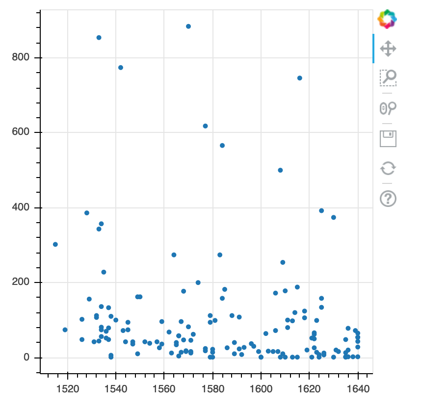
Building your plots
We can add extra arguments into circle’s argument.
For comparison, we create a new figure and then add the alpha argument to circle to change the opacity of the points.
PYTHON
p1 = figure(plot_width=400, plot_height=400)

p1.circle(list_dates, list_numbers, alpha=0.1)

show(p1)
We can also add colors for all the points.
PYTHON
p2 = figure(plot_width=400, plot_height=400)

p2.circle(list_dates, list_numbers, color="blue", alpha=0.1)

show(p2)
Plotting time series data
Let’s calculate number of counts per year across the dataset. To do that we need to group data first and count records within each group.
PYTHON
yearly = authors_df[['Date','Place','Page Count']].groupby(['Date', 'Place']).count().reset_index()PYTHON
p3 = figure(plot_width=800, plot_height=250)

p3.line(yearly['Date'], yearly['Page Count'], color='navy', alpha=0.5)

show(p3)
year place count0 1515 London 1 1 1519 Londini 1 2 1526 London 2 3 1528 London 1 4 1529 Malborow i.e. Antwerp 1 5 1531 London 1
[121 rows x 3 columns]
Timelapse data can be visualised as a line plot with years on x axis and counts on y axis.
p3 = figure(plot_width=800, plot_height=250)
p3.line(yearly['Date'], yearly['Page Count'], color='navy', alpha=0.5)
show(p3)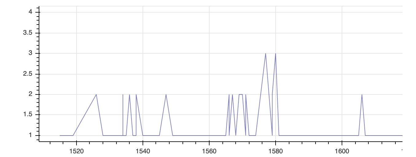
Customization
Now, let’s add a title to this figure:
PYTHON
from bokeh.models import ColumnDataSource, Range1d, LabelSet, Label

p4 = figure(title="Plot of Page Counts by Year", plot_width=400, plot_height=400)

p4.circle(list_dates, list_numbers)

p4.xaxis[0].axis_label = 'Date'
p4.yaxis[0].axis_label = 'Page Count'

show(p4)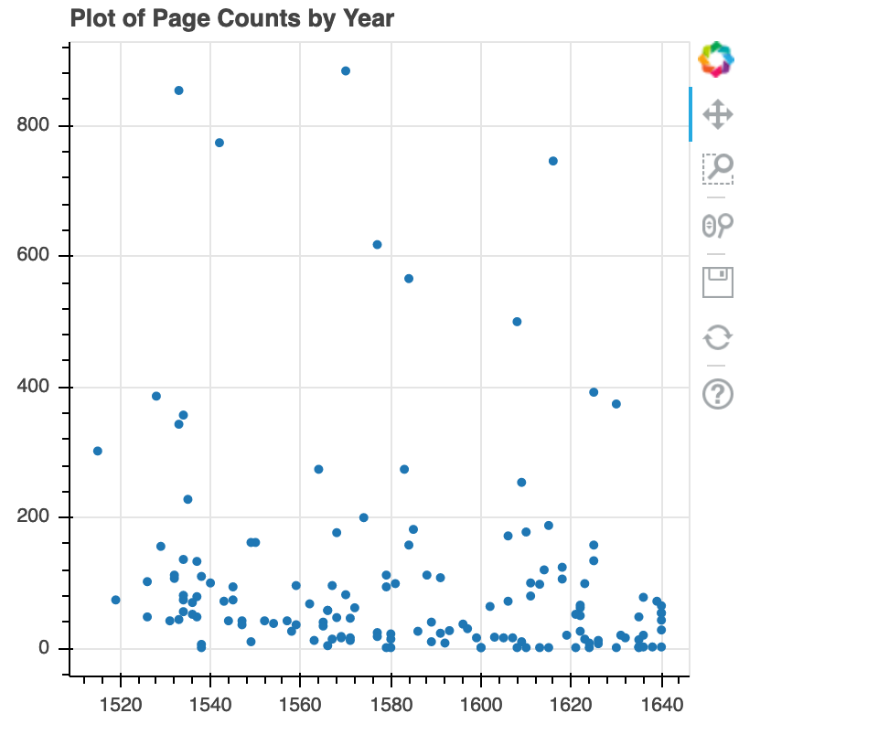
or we canadd labels to the axes and change the font size for the labels
PYTHON
p5 = figure(title="Plot of Page Counts by Year", plot_width=400, plot_height=400)

p5.circle(list_dates, list_numbers)

p5.xaxis[0].axis_label = 'Date'
p5.yaxis[0].axis_label = 'Page Count'
p5.xaxis[0].axis_label_text_font_size = "24pt"

show(p5)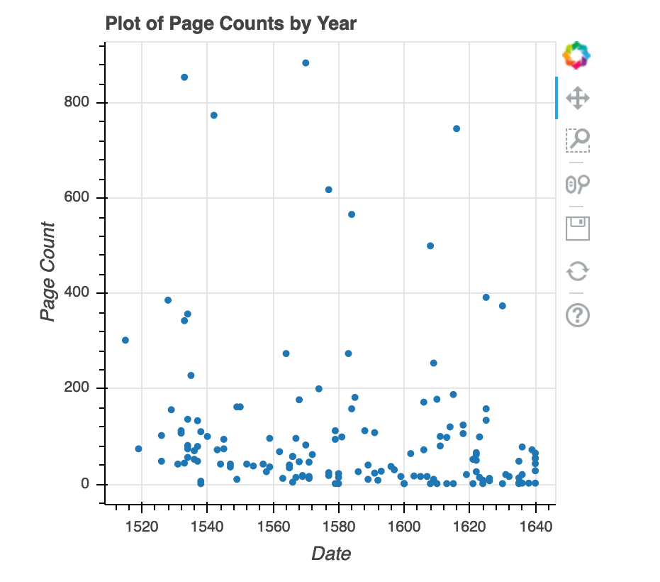
With all of this information in hand, please take another five minutes to either improve one of the plots generated in this exercise or create a beautiful graph of your own.
Here are some ideas:
- Can you find a way to change its labels?
- Use a different color palette.
After creating your plot, you can save it to a file as a png file:
Content from Data Ingest & Visualization - Matplotlib & Pandas
Last updated on 2024-02-13 | Edit this page
Overview
Questions
- What other tools can I use to create plots apart from ggplot?
- Why should I use Python to create plots?
Objectives
- Import the pyplot toolbox to create figures in Python.
Putting it all together
Up to this point, we have walked through tasks that are often
involved in handling and processing data using the workshop ready
cleaned
files that we have provided. In this wrap-up exercise, we will perform
many of the same tasks with real data sets. This lesson also covers data
visualization.
As opposed to the previous ones, this lesson does not give step-by-step directions to each of the tasks. Use the lesson materials you’ve already gone through as well as the Python documentation to help you along.
1. Obtain data
There are many repositories online from which you can obtain data. We
are providing you with one data file to use with these exercises, but
feel free to use any data that is relevant to your research. The file
eebo.csv contains the complete EEBO metadata of books
between 1300-1700. If you’d like to use this dataset, please find it in
the data folder.
2. Clean up your data and open it using Python and Pandas
To begin, import your data file into Python using Pandas. Did it fail? Your data file probably has a header that Pandas does not recognize as part of the data table. Remove this header, but do not simply delete it in a text editor! Use either a shell script or Python to do this - you wouldn’t want to do it by hand if you had many files to process.
If you are still having trouble importing the data as a table using Pandas, check the documentation. You can open the docstring in an ipython notebook using a question mark. For example:
Look through the function arguments to see if there is a default
value that is different from what your file requires (Hint: the problem
is most likely the delimiter or separator. Common delimiters are
',' for comma, ' ' for space, and
'\t' for tab).
Create a DataFrame that includes only the values of the data that are useful to you. In the streamgage file, those values might be the date, title, terms, and TCP. Convert and joined strings into individual ones. You can also change the name of the columns in the DataFrame like this:
PYTHON
    df['Author'] = df['Author'].str.split(';') #split a column in the data frame

    df = pd.DataFrame({'1stcolumn':[100,200], '2ndcolumn':[10,20]}) # this just creates a DataFrame for the example!
    print('With the old column names:\n') # the \n makes a new line, so it's easier to see
    print(df)

    df.columns = ['FirstColumn','SecondColumn'] # rename the columns!
    print('\n\nWith the new column names:\n')
    print(df)

    With the old column names:

       1stcolumn  2ndcolumn
    0        100         10
    1        200         20


    With the new column names:

       FirstColumn  SecondColumn
    0          100            10
    1          200            20
3. Make a line plot of your data
Matplotlib is a Python library that can be used to visualize data.
The toolbox matplotlib.pyplot is a collection of functions
that make matplotlib work like MATLAB. In most cases, this is all that
you will need to use, but there are many other useful tools in
matplotlib that you should explore.
We will cover a few basic commands for formatting plots in this lesson. A great resource for help styling your figures is the matplotlib gallery (http://matplotlib.org/gallery.html), which includes plots in many different styles and the source code that creates them. The simplest of plots is the 2 dimensional line plot. These examples walk through the basic commands for making line plots using pyplots.
Challenge - Lots of plots
Make a variety of line plots from your data. If you are using the
streamgage data, these could include (1) a hydrograph of the entire
month of September 2013, (2) the discharge record for the week of the
2013 Front Range flood (September 9 through 15), (3) discharge vs. time
of day, for every day in the record in one figure (Hint: use loops to
combine strings and give every line a different style and color), and
(4) minimum, maximum, and mean daily discharge values. Add axis labels,
titles, and legends to your figures. Make at least one figure with
multiple plots using the function subplot().
Using pyplot:
First, import the pyplot toolbox:
By default, matplotlib will create the figure in a separate window. When using ipython notebooks, we can make figures appear in-line within the notebook by writing:
We can start by plotting the values of a list of numbers (matplotlib can handle many types of numeric data, including numpy arrays and pandas DataFrames - we are just using a list as an example!):
The command plt.show() prompts Python to display the
figure. Without it, it creates an object in memory but doesn’t produce a
visible plot. The ipython notebooks (if using
%matplotlib inline) will automatically show you the figure
even if you don’t write plt.show(), but get in the habit of
including this command!
If you provide the plot() function with only one list of
numbers, it assumes that it is a sequence of y-values and plots them
against their index (the first value in the list is plotted at
x=0, the second at x=1, etc). If the function
plot() receives two lists, it assumes the first one is the
x-values and the second the y-values. The line connecting the points
will follow the list in order:
A third, optional argument in plot() is a string of
characters that indicates the line type and color for the plot. The
default value is a continuous blue line. For example, we can make the
line red ('r'), with circles at every data point
('o'), and a dot-dash pattern ('-.'). Look
through the matplotlib gallery for more examples.
The command plt.axis() sets the limits of the axes from
a list of [xmin, xmax, ymin, ymax] values (the square
brackets are needed because the argument for the function
axis() is one list of values, not four separate numbers!).
The functions xlabel() and ylabel() will label
the axes, and title() will write a title above the
figure.
A single figure can include multiple lines, and they can be plotted
using the same plt.plot() command by adding more pairs of x
values and y values (and optionally line styles):
PYTHON
    import numpy as np

    # create a numpy array between 0 and 10, with values evenly spaced every 0.5
    t = np.arange(0., 10., 0.5)

    # red dashes with no symbols, blue squares with a solid line, and green triangles with a dotted line
    plt.plot(t, t, 'r--', t, t**2, 'bs-', t, t**3, 'g^:')

    plt.xlabel('This is the x axis')
    plt.ylabel('This is the y axis')
    plt.title('This is the figure title')

    plt.show()
We can include a legend by adding the optional keyword argument
label='' in plot(). Caution: We cannot add
labels to multiple lines that are plotted simultaneously by the
plt.plot() command like we did above because Python won’t
know to which line to assign the value of the argument label. Multiple
lines can also be plotted in the same figure by calling the
plot() function several times:
PYTHON
    # red dashes with no symbols, blue squares with a solid line, and green triangles with a dotted line
    plt.plot(t, t, 'r--', label='linear')
    plt.plot(t, t**2, 'bs-', label='square')
    plt.plot(t, t**3, 'g^:', label='cubic')

    plt.legend(loc='upper left', shadow=True, fontsize='x-large')

    plt.xlabel('This is the x axis')
    plt.ylabel('This is the y axis')
    plt.title('This is the figure title')

    plt.show()
The function legend() adds a legend to the figure, and
the optional keyword arguments change its style. By default [typing just
plt.legend()], the legend is on the upper right corner and
has no shadow.
Like MATLAB, pyplot is stateful; it keeps track of the current figure
and plotting area, and any plotting functions are directed to those
axes. To make more than one figure, we use the command
plt.figure() with an increasing figure number inside the
parentheses:
PYTHON
    # this is the first figure
    plt.figure(1)
    plt.plot(t, t, 'r--', label='linear')

    plt.legend(loc='upper left', shadow=True, fontsize='x-large')
    plt.title('This is figure 1')

    plt.show()

    # this is a second figure
    plt.figure(2)
    plt.plot(t, t**2, 'bs-', label='square')

    plt.legend(loc='upper left', shadow=True, fontsize='x-large')
    plt.title('This is figure 2')

    plt.show()
A single figure can also include multiple plots in a grid pattern.
The subplot() command especifies the number of rows, the
number of columns, and the number of the space in the grid that
particular plot is occupying:
PYTHON
    plt.figure(1)

    plt.subplot(2,2,1) # two row, two columns, position 1
    plt.plot(t, t, 'r--', label='linear')

    plt.subplot(2,2,2) # two row, two columns, position 2
    plt.plot(t, t**2, 'bs-', label='square')

    plt.subplot(2,2,3) # two row, two columns, position 3
    plt.plot(t, t**3, 'g^:', label='cubic')

    plt.show()
4. Make other types of plots:
Matplotlib can make many other types of plots in much the same way
that it makes 2 dimensional line plots. Look through the examples in http://matplotlib.org/users/screenshots.html
and try a few of them (click on the “Source code” link and copy and
paste into a new cell in ipython notebook or save as a text file with a
.py extension and run in the command line).
Challenge - Final Plot
Display your data using one or more plot types from the example gallery. Which ones to choose will depend on the content of your own data file. If you are using the streamgage file, you could make a histogram of the number of days with a given mean discharge, use bar plots to display daily discharge statistics, or explore the different ways matplotlib can handle dates and times for figures.
Content from Accessing SQLite Databases Using Python & Pandas
Last updated on 2024-02-13 | Edit this page
Python and SQL
When you open a CSV in python, and assign it to a variable name, you are using your computers memory to save that variable. Accessing data from a database like SQL is not only more efficient, but also it allows you to subset and import only the parts of the data that you need.
In the following lesson, we’ll see some approaches that can be taken to do so.
The sqlite3 module
The sqlite3 module
provides a straightforward interface for interacting with SQLite
databases. A connection object is created using
sqlite3.connect(); the connection must be closed at the end
of the session with the .close() command. While the
connection is open, any interactions with the database require you to
make a cursor object with the .cursor() command. The cursor
is then ready to perform all kinds of operations with
.execute().
Queries
One of the most common ways to interact with a database is by querying: retrieving data based on some search parameters. Use a SELECT statement string. The query is returned as a single tuple or a tuple of tuples. Add a WHERE statement to filter your results based on some parameter.
PYTHON
import sqlite3

# Create a SQL connection to our SQLite database
con = sqlite3.connect("eebo.db")

cur = con.cursor()

# Return all results of query
cur.execute('SELECT Title FROM eebo WHERE Status="Free"')
cur.fetchall()

# Return first result of query
cur.execute('SELECT Title FROM eebo WHERE Status="Free"')
cur.fetchone()

#Be sure to close the connection.
con.close()
Accessing data stored in SQLite using Python and Pandas
Using pandas, we can import results of a SQLite query into a dataframe. Note that you can use the same SQL commands / syntax that we used in the SQLite lesson. An example of using pandas together with sqlite is below:
Storing data: CSV vs SQLite
Storing your data in an SQLite database can provide substantial performance improvements when reading/writing compared to CSV. The difference in performance becomes more noticable as the size of the dataset grows (see for example these benchmarks).
Challenge - SQL
- Create a query that contains title data published between 1550 - 1650 that includes book’s Title, Author, and TCP id. How many records are returned?
Storing data: Create new tables using Pandas
We can also us pandas to create new tables within an SQLite database. Here, we run we re-do an excercise we did before with CSV files using our SQLite database. We first read in our survey data, then select only those survey results for 2002, and then save it out to its own table so we can work with it on its own later.
PYTHON
import pandas as pd
import sqlite3

con = sqlite3.connect("eebo.db")

# Load the data into a DataFrame
books_df = pd.read_sql_query("SELECT * from eebo", con)

# Select only data for 1640
titles1640 = books_df[books_df.Date == '1640']

# Write the new DataFrame to a new SQLite table
titles1640.to_sql("titles1640", con, if_exists="replace")

con.close()Challenge - Saving your work
For each of the challenges in the previous challenge block, modify your code to save the results to their own tables in the eebo database.
What are some of the reasons you might want to save the results of your queries back into the database? What are some of the reasons you might avoid doing this.