Content from Introduction
Last updated on 2023-08-29 | Edit this page
Estimated time: 30 minutes
Overview
Questions
- How do you build machine learning pipelines for time-series analysis?
Objectives
- Introduce machine learning concepts applicable to time-series forecasting.
- Introduce Google’s
TensorFlowmachine learning library for Python.
Introduction
This lesson is the third in a series of lessons demonstrating Python libraries and methods for time-series analysis and forecasting.
The first lesson, Time
Series Analysis of Smart Meter Power Consmption Data, introduces
datetime indexing features in the Python Pandas library.
Other topics in the lesson include grouping data, resampling by time
frequency, and plotting rolling averages.
The second lesson, Modeling Power Consumption with Python, introduces the component processes of the SARIMAX model for single-step forecasts based on a single variable.
This lesson builds upon the first two by applying machine learning processes to build models with potentially greater predictive power against larger datasets. Relevant concepts include:
- Feature engineering
- Data windows
- Single step forecasts
- Multi-step forecasts
Throughout, the lesson uses Google’s TensorFlow machine
learning library and the related Python API, keras. As
noted in each section of the lesson, the code is based upon and is in
many cases a direct implementation of the Time
series forecasting tutorial available from the TensorFlow
project. Per the documentation, materials available from the TensorFlow
GitHub site are published using an Apache
2.0 license.
Google Inc. (2023) TensorFlow Documentation. Retrieved from https://github.com/tensorflow/docs/blob/master/README.md.
This lesson uses the same dataset as the previous two. For more information about the data, see the Setup page.
Key Points
- The
TensorFlowmachine learning library from Google provides many algorithms and models for efficient pipelines to process and forecast large time-series datasets.
Content from Feature Engineering
Last updated on 2023-08-25 | Edit this page
Estimated time: 50 minutes
Overview
Questions
- How do you prepare time-series data for machine learning?
Objectives
- Extract datetime elements from a Pandas datetime index.
Introduction
Machine learning methods can fall into two broad categories
- supervised
- unsupervised.
In both cases, the affect or influence of one or more features of an observation are analyzed to determine their effect on a result. The result in this case is termed a label. In supervised learning techniques, models are trained using pre-labeled data. The labels in this case act as a ground truth against which a model’s performance can be compared and evaluated.
In an unsupervised learning process, models are trained using data for which ground truth labels have not been identified. Ground truth in these cases is determined statistically.
Throughout this lesson we are going to focus on unsupervised machine learning techniques to forecast power consumption.
About the code
The code for this and other sections of this lesson is based on time-series forecasting examples, tutorials, and other documentation available from the TensorFlow project. Per the documentation, materials available from the TensorFlow GitHub site published using an Apache 2.0 license.
Google Inc. (2023) TensorFlow Documentation. Retrieved from https://github.com/tensorflow/docs/blob/master/README.md.
Features
The data we used in a separate lesson on modeling time-series forecasts, and which we will continue to use here, include a handful of variables:
- INTERVAL_TIME
- METER_FID
- START_READ
- END_READ
- INTERVAL_READ
In these previous analyses, the only variable used for forecasting power consumption were INTERVAL_READ and INTERVAL_TIME. Going forward, we can capitalize on the efficiency and accuracy of machine learning methods via feature engineering. That is, we want to identify and include as many time-based features as possible that may be relevant to power consumption. For example, though some of our previous models accounted for seasonal trends in the data, other factors that influence power consumption were more difficult to include in our models:
- Day of the week
- Business days, weekends, and holidays
- Season
While some of these features were implicit in the data - for example, power consumption during the US summer notably increased - making these features explicit in our data can result in more accurate machine learning models, with more predictive power.
In this section, we demonstrate a process for extracting these features from a datetime index. The dataset output at the end of this section will be used throughout the rest of this lesson for making forecasts.
Read data
To begin with, import the necessary libraries. We will introduce some new libraries in later sections, but here we only need a handful of libraries to pre-process our daa.
Next we read the data, and set and sort the datetime index.
PYTHON
fp = "../../data/ladpu_smart_meter_data_07.csv"
df = pd.read_csv(fp)
df.set_index(pd.to_datetime(df["INTERVAL_TIME"]), inplace=True)
df.sort_index(inplace=True)
print(df.info())
print(df.index)OUTPUT
<class 'pandas.core.frame.DataFrame'>
DatetimeIndex: 105012 entries, 2017-01-01 00:00:00 to 2019-12-31 23:45:00
Data columns (total 5 columns):
# Column Non-Null Count Dtype
--- ------ -------------- -----
0 INTERVAL_TIME 105012 non-null object
1 METER_FID 105012 non-null int64
2 START_READ 105012 non-null float64
3 END_READ 105012 non-null float64
4 INTERVAL_READ 105012 non-null float64
dtypes: float64(3), int64(1), object(1)
memory usage: 4.8+ MB
None
DatetimeIndex(['2017-01-01 00:00:00', '2017-01-01 00:15:00',
'2017-01-01 00:30:00', '2017-01-01 00:45:00',
'2017-01-01 01:00:00', '2017-01-01 01:15:00',
'2017-01-01 01:30:00', '2017-01-01 01:45:00',
'2017-01-01 02:00:00', '2017-01-01 02:15:00',
...
'2019-12-31 21:30:00', '2019-12-31 21:45:00',
'2019-12-31 22:00:00', '2019-12-31 22:15:00',
'2019-12-31 22:30:00', '2019-12-31 22:45:00',
'2019-12-31 23:00:00', '2019-12-31 23:15:00',
'2019-12-31 23:30:00', '2019-12-31 23:45:00'],
dtype='datetime64[ns]', name='INTERVAL_TIME', length=105012, freq=None)We will forecasting hourly power consumption in later sections, so we need to resample the data to an hourly frequency here.
PYTHON
hourly_readings = pd.DataFrame(df.resample("h")["INTERVAL_READ"].sum())
print(hourly_readings.info())
print(hourly_readings.head())OUTPUT
<class 'pandas.core.frame.DataFrame'>
DatetimeIndex: 26280 entries, 2017-01-01 00:00:00 to 2019-12-31 23:00:00
Freq: H
Data columns (total 1 columns):
# Column Non-Null Count Dtype
--- ------ -------------- -----
0 INTERVAL_READ 26280 non-null float64
dtypes: float64(1)
memory usage: 410.6 KB
None
INTERVAL_READ
INTERVAL_TIME
2017-01-01 00:00:00 1.4910
2017-01-01 01:00:00 0.3726
2017-01-01 02:00:00 0.3528
2017-01-01 03:00:00 0.3858
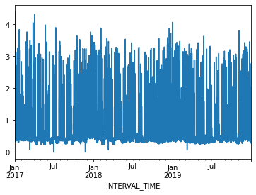
2017-01-01 04:00:00 0.4278A plot of the entire dataset is somewhat noisy, though seasonal trends are apparent.
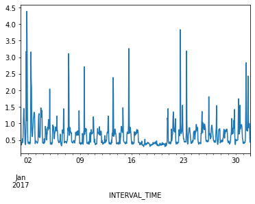
Ploting hourly consumption for the month of January, 2017, is less noisy though there are no obvious trends in the data.
Finally, before manipulating the data we can inspect for anomalies or
outliers using descriptive statistics. Even though we only have a single
variable to describe in our current dataset, the
transpose() method used below is useful in cases where you
want to tabulate descriptive statistics for multiple variables.
OUTPUT
count mean std min 25% 50% 75% max
INTERVAL_READ 26280.0 0.624122 0.405971 0.0 0.3714 0.4818 0.756 4.3872The max value of 4.3872 may seem like an outlier,
considering that 75% of INTERVAL_READ values are 0.4818 or less.
However, a look back up to our first plot indicates peak power
consumption over a relatively short time period in the middle of the
year. For now we will accept this max value as reasonable.
Add datetime features
Most of the features that we will add to the data are attributes of datetime objects in Pandas. We can extract them using their attribute names:
PYTHON
print("hour:", hourly_readings.head().index.hour)
print("day of the month:", hourly_readings.head().index.day)
print("day of week:", hourly_readings.head().index.day_of_week)
print("day of year:", hourly_readings.head().index.day_of_year)
print("day name:", hourly_readings.head().index.day_name())
print("week of year:",hourly_readings.head().index.week)
print("month:", hourly_readings.head().index.month)
print("year", hourly_readings.head().index.year)OUTPUT
hour: Int64Index([0, 1, 2, 3, 4], dtype='int64', name='INTERVAL_TIME')
day of the month: Int64Index([1, 1, 1, 1, 1], dtype='int64', name='INTERVAL_TIME')
day of week: Int64Index([6, 6, 6, 6, 6], dtype='int64', name='INTERVAL_TIME')
day of year: Int64Index([1, 1, 1, 1, 1], dtype='int64', name='INTERVAL_TIME')
day name: Index(['Sunday', 'Sunday', 'Sunday', 'Sunday', 'Sunday'], dtype='object', name='INTERVAL_TIME')
week of year: Int64Index([52, 52, 52, 52, 52], dtype='int64', name='INTERVAL_TIME')
month: Int64Index([1, 1, 1, 1, 1], dtype='int64', name='INTERVAL_TIME')
year Int64Index([2017, 2017, 2017, 2017, 2017], dtype='int64', name='INTERVAL_TIME')We can add these attributes as new features. Out of the attributes shown above, we are only going to add a few numeric types and a full date string.
PYTHON
hourly_readings['hour'] = hourly_readings.index.hour
hourly_readings['day_month'] = hourly_readings.index.day
hourly_readings['day_week'] = hourly_readings.index.day_of_week
hourly_readings['month'] = hourly_readings.index.month
hourly_readings['date'] = hourly_readings.index.to_series().apply(lambda x: x.strftime("%Y-%m-%d"))
print(hourly_readings.info())
print(hourly_readings.head())
print(hourly_readings.tail())OUTPUT
<class 'pandas.core.frame.DataFrame'>
DatetimeIndex: 26280 entries, 2017-01-01 00:00:00 to 2019-12-31 23:00:00
Freq: H
Data columns (total 6 columns):
# Column Non-Null Count Dtype
--- ------ -------------- -----
0 INTERVAL_READ 26280 non-null float64
1 hour 26280 non-null int64
2 day_month 26280 non-null int64
3 day_week 26280 non-null int64
4 month 26280 non-null int64
5 date 26280 non-null object
dtypes: float64(1), int64(4), object(1)
memory usage: 1.4+ MB
None
INTERVAL_READ hour ... month date
INTERVAL_TIME ...
2017-01-01 00:00:00 1.4910 0 ... 1 2017-01-01
2017-01-01 01:00:00 0.3726 1 ... 1 2017-01-01
2017-01-01 02:00:00 0.3528 2 ... 1 2017-01-01
2017-01-01 03:00:00 0.3858 3 ... 1 2017-01-01
2017-01-01 04:00:00 0.4278 4 ... 1 2017-01-01
[5 rows x 6 columns]
INTERVAL_READ hour ... month date
INTERVAL_TIME ...
2019-12-31 19:00:00 0.7326 19 ... 12 2019-12-31
2019-12-31 20:00:00 0.7938 20 ... 12 2019-12-31
2019-12-31 21:00:00 0.7878 21 ... 12 2019-12-31
2019-12-31 22:00:00 0.7716 22 ... 12 2019-12-31
2019-12-31 23:00:00 0.4986 23 ... 12 2019-12-31
[5 rows x 6 columns]Another feature than can influence power consumption is whether a
given day is a business day, a weekend, or a holiday. For our purposes,
since our data only span three years there may not be enough holidays to
include those as a specific feature. However, we can include US federal
holidays in a customized calendar of business days using Pandas’
holiday and offsets methods.
Note that while this example uses the US federal holiday calendar, Pandas includes holidays and other business day offsets for other regions and locales.
PYTHON
from pandas.tseries.holiday import USFederalHolidayCalendar
from pandas.tseries.offsets import CustomBusinessDay
us_bus = CustomBusinessDay(calendar=USFederalHolidayCalendar())
# Set the business day date range to the start and end dates of our data
us_business_days = pd.bdate_range('2017-01-01', '2019-12-31', freq=us_bus)
hourly_readings["business_day"] = pd.to_datetime(hourly_readings["date"]).isin(us_business_days)
print(hourly_readings.info())OUTPUT
<class 'pandas.core.frame.DataFrame'>
DatetimeIndex: 26280 entries, 2017-01-01 00:00:00 to 2019-12-31 23:00:00
Freq: H
Data columns (total 7 columns):
# Column Non-Null Count Dtype
--- ------ -------------- -----
0 INTERVAL_READ 26280 non-null float64
1 hour 26280 non-null int64
2 day_month 26280 non-null int64
3 day_week 26280 non-null int64
4 month 26280 non-null int64
5 date 26280 non-null object
6 business_day 26280 non-null bool
dtypes: bool(1), float64(1), int64(4), object(1)
memory usage: 1.4+ MB
NoneWe want to pass numeric data types to the machine learning processes covered in later sections, so we’ll convert the boolean (True and False) values for business_day to integers (1 for True and 0 for False).
PYTHON
hourly_readings = hourly_readings.astype({"business_day": "int"})
print(hourly_readings.dtypes)OUTPUT
INTERVAL_READ float64
hour int64
day_month int64
day_week int64
month int64
date object
day_sin float64
day_cos float64
business_day int32
dtype: objectSine and cosine transformation
Finally, we can apply a sine and cosine transformation to some of the datetime features to more effectively represent the cyclic or periodic nature of specific time frequencies.
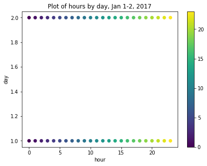
For example, though we have added an hour feature, the data are ordinal. That is, the values for each hour go from 1-24 in order, but hours as an ordinal feature don’t express a cyclic relationship relative to the idea that 1:00 AM of a given date is, time-wise, more or less similar to 1:00 AM of the day before or after. For example, the figure below is a scatter plot of hours per day for January 1-2, 2017, in which ordinal hour “values” are plotted against ordinal day “values.” The overlap we might expect from one day ending and another beginning is not represented.
We can use sine and cosine transformations to add features that capture this characteristic of time. First, we create a timestamp series based on the datetime index.
OUTPUT
Float64Index([1483228800.0, 1483232400.0, 1483236000.0, 1483239600.0,
1483243200.0, 1483246800.0, 1483250400.0, 1483254000.0,
1483257600.0, 1483261200.0,
...
1577800800.0, 1577804400.0, 1577808000.0, 1577811600.0,
1577815200.0, 1577818800.0, 1577822400.0, 1577826000.0,
1577829600.0, 1577833200.0],
dtype='float64', name='INTERVAL_TIME', length=26280)Since timestamps are counted per second, next we want to calculate the number of timestamps in a day and in a year. These values are then applied to sine and cosine transformations of each timestamp value. The transformed values are added as new features to the dataset.
Note that we could use a similar process for weeks, or other datetime elements.
PYTHON
day = 24*60*60
year = (365.2425)*day
hourly_readings['day_sin'] = np.sin(ts_s * (2 * np.pi / day))
hourly_readings['day_cos'] = np.cos(ts_s * (2 * np.pi / day))
hourly_readings['year_sin'] = np.sin(ts_s * (2 * np.pi / year))
hourly_readings['year_cos'] = np.cos(ts_s * (2 * np.pi / year))
print(hourly_readings.info())OUTPUT
<class 'pandas.core.frame.DataFrame'>
DatetimeIndex: 26280 entries, 2017-01-01 00:00:00 to 2019-12-31 23:00:00
Freq: H
Data columns (total 9 columns):
# Column Non-Null Count Dtype
--- ------ -------------- -----
0 INTERVAL_READ 26280 non-null float64
1 hour 26280 non-null int64
2 day_month 26280 non-null int64
3 day_week 26280 non-null int64
4 month 26280 non-null int64
5 date 26280 non-null object
6 business_day 26280 non-null bool
7 day_sin 26280 non-null float64
8 day_cos 26280 non-null float64
dtypes: bool(1), float64(3), int64(4), object(1)
memory usage: 1.8+ MB
NoneIf we now plot the transformed values for January 1-2, 2017, we can see that the plot has a clock-like appearance and that the values for the different hours overlap. In fact, although this is only a plot of the first 48 hours, we could plot the entire dataset and the plot would look the same.
fig, ax = plt.subplots(figsize=(7, 5))
sp = ax.scatter(hourly_readings[:48]['day_sin'],
hourly_readings[:48]['day_cos'],
c = hourly_readings[:48]['hour'])
ax.set(
xlabel="sin(hour)",
ylabel="cos(hour)",
title="Plot of hours by day, Jan 1-2, 2017"
)
_ = fig.colorbar(sp)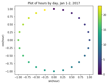
Export data to CSV
At this point, we have added several datetime features to our dataset using datetime attributes. We have additionally used these attributes to add sine and cosine transformed hour features, and a boolean feature indicating whether or not any given day in the dataset is a business day.
Rather than redo this process for the remaining sections of this lesson, we will export the current dataset for later use. The file will be saved to the data directory referenced in the Setup section of this lesson.
Key Points
- Use sine and cosine transformations to represent the periodic or cyclical nature of time-series data.
Content from Data Windowing and Making Datasets
Last updated on 2023-08-28 | Edit this page
Estimated time: 50 minutes
Overview
Questions
- How do we prepare time-series datasets for machine learning?
Objectives
- Explain data windows and dataset slicing with TensorFlow.
- Create training, validation, and test datasets for analysis.
Introduction
Before making forecasts with our time-series data, we need to create training, validation, and test datasets. While this process is similar to that which was demonstrated in a previous lesson on the SARIMAX model, in addition to adding a validation dataset, a key difference with unsupervised machine learning is the definition of data windows.
Returning to our earlier definition of features and labels, a data window defines the attributes of a slice or batch of features and labels from a dataset that are the inputs to a machine learning process. These attributes specify:
- the number of time steps in the slice
- the number of time steps which are inputs and labels
- the time step offset between inputs and labels
- input and label features.
As we will see in later sections, data windows can be used to make both single and multi-step forecasts. They can also be used to predict one or more labels, though that will not be covered in this lesson since our primary focus is forecasting a single feature within our time-series: power consumption.
In this section, we will create training, validation, and test datasets using normalized data. We will then progressively build and demonstrate a class for creating data windows and datasets.
About the code
The code for this and other sections of this lesson is based on time-series forecasting examples, tutorials, and other documentation available from the TensorFlow project. Per the documentation, materials available from the TensorFlow GitHub site published using an Apache 2.0 license.
Google Inc. (2023) TensorFlow Documentation. Retrieved from https://github.com/tensorflow/docs/blob/master/README.md.
Read and split data
First, import the necessary libraries.
PYTHON
import os
import matplotlib as mpl
import matplotlib.pyplot as plt
import numpy as np
import pandas as pd
import seaborn as sns
import tensorflow as tfIn the previous section of this lesson, we extracted multiple datetime attributes in order to add relevant features to our dataset. In the course of developing this lesson, multiple combinations of features were tested against different models to determine which combination provides the best performance without overfitting the models. The features we will use are
- INTERVAL_READ
- hour
- day_sin
- day_cos
- business_day
We will keep these features in our pre-processed smart meter dataset, but drop them after reading the data. You are encouraged to test different combinations of features against our models!
PYTHON
df = pd.read_csv('../../data/hourly_readings.csv')
drop_cols = ["INTERVAL_TIME", "date", "month", "day_month", "day_week"]
df.drop(drop_cols, axis=1, inplace=True)
print(df.info())
print(df.head())
OUTPUT
<class 'pandas.core.frame.DataFrame'>
RangeIndex: 26280 entries, 0 to 26279
Data columns (total 5 columns):
 #   Column         Non-Null Count  Dtype
---  ------         --------------  -----
 0   INTERVAL_READ  26280 non-null  float64
 1   hour           26280 non-null  int64
 2   day_sin        26280 non-null  float64
 3   day_cos        26280 non-null  float64
 4   business_day   26280 non-null  int64
dtypes: float64(3), int64(2)
memory usage: 1.0 MB
None


   INTERVAL_READ  hour       day_sin   day_cos  business_day
0         1.4910     0  2.504006e-13  1.000000             0
1         0.3726     1  2.588190e-01  0.965926             0
2         0.3528     2  5.000000e-01  0.866025             0
3         0.3858     3  7.071068e-01  0.707107             0
4         0.4278     4  8.660254e-01  0.500000             0
Next, we split the dataset into training, validation, and test sets. The size of the training data will be 70% of the source data. The sizes of the validation and test datasets will be 20% and 10% of the source data, respectively.
It is not unusual when creating training, validation, and test datasets to randomly shuffle the data before splitting. In the case of time-series, we do not do this because in order to make meaningful forecasts it is important to maintain the order of the data.
PYTHON
n = len(df)
train_df = df[0:int(n*0.7)]
val_df = df[int(n*0.7): int(n*0.9)]
test_df = df[int(n*0.9):]

print("Training length:", len(train_df))
print("Validation length:", len(val_df))
print("Test length:", len(test_df))
OUTPUT
Training length: 18396
Validation length: 5256
Test length: 2628
Scale the data
Scaling the data normalizes the distributions of values across features. This allows for more efficient modeling. We can see the effect of normalizing the data by plotting the distribution before and after scaling.
PYTHON
df_non = df.copy()
df_non = df_non.melt(var_name='Column', value_name='Non-normalized')

plt.figure(figsize=(12, 6))
ax = sns.violinplot(x='Column', y='Non-normalized', data=df_non)
_ = ax.set_xticklabels(df.keys(), rotation=90)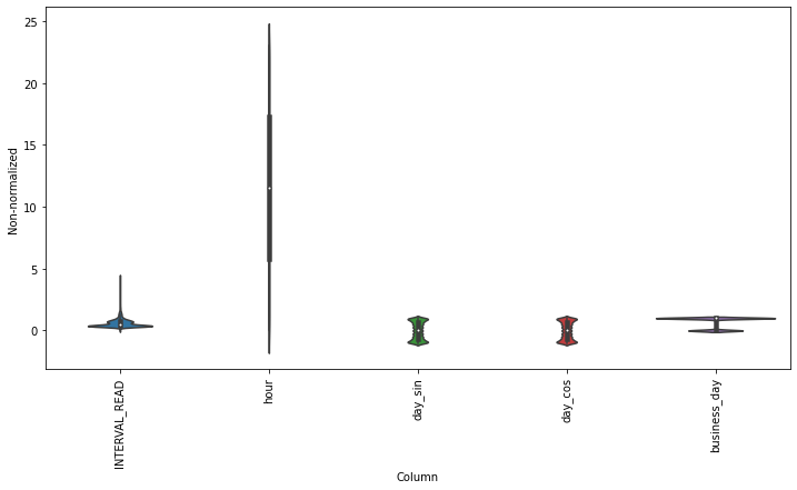
We scale the data by subtracting the mean of the training data and then dividing the result by the standard deviation of the training data. Rather than create new dataframes, we will overwrite the existing source data with the normalized values.
PYTHON
train_mean = train_df.mean()
train_std = train_df.std()

train_df = (train_df - train_mean) / train_std
val_df = (val_df - train_mean) / train_std
test_df = (test_df - train_mean) / train_std
Plotting the scaled data demonstrates the normalized distributions.
PYTHON
df_std = (df - train_mean) / train_std
df_std = df_std.melt(var_name='Col', value_name='Normalized')
plt.figure(figsize=(12, 6))
ax = sns.violinplot(x='Col', y='Normalized', data=df_std)
_ = ax.set_xticklabels(df.keys(), rotation=90)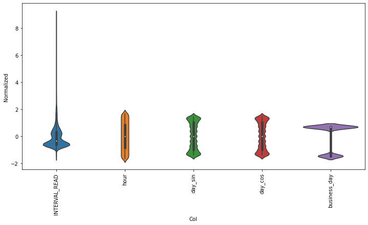
Rather than go through the process of reading, splitting, and normalizing the data in each section of this lesson, let’s save the training, validation, and test datasets for later use.
Instantiate data windows
As briefly described above, data windows are slices of the training
dataset that are passed to a machine learning model for fitting and
evaluation. Below, we define a WindowGenerator class that
is capable of flexible window and dataset creation and which we will
apply later to both single and multi- step forecasts.
The WindowGenerator code as provided here is as given in
Google’s TensorFlow documentation, referenced above.
Because windows are slices of a dataset, it is necessary to determine the index positions of the rows that will be included in a window. The necessary class attributes are defined in the initialization function of the class:
- input_width is the width or number of timesteps to use as the history of previous values on which a forecast is based
- label_width is the number of timesteps that will be forecast
- shift defines how many timesteps ahead a forecast is being made
The training, validation, and test dataframes created above are
passed as default arguments when a WindowGenerator object
is instantiated. This allows the object to access the data without
having to specify which datasets to use every time a new data window is
created or a model is fitted.
Finally, an optional keyword argument, label_columns, allows us to identify which features are being modeled. It is possible to forecast more than one feature, but as noted above that is beyond the scope of this lesson. Note that it is possible to instantiate a data window without specifying the features that will be predicted.
PYTHON
class WindowGenerator():
  def __init__(self, input_width, label_width, shift,
               train_df=train_df, val_df=val_df, test_df=test_df,
               label_columns=None):
    # Make the raw data available to the data window.
    self.train_df = train_df
    self.val_df = val_df
    self.test_df = test_df

    # Get the column index positions of the label features.
    self.label_columns = label_columns
    if label_columns is not None:
      self.label_columns_indices = {name: i for i, name in
                                    enumerate(label_columns)}
    self.column_indices = {name: i for i, name in
                           enumerate(train_df.columns)}

    # Get the row index positions of the full window, the inputs,
    # and the label(s).
    self.input_width = input_width
    self.label_width = label_width
    self.shift = shift

    self.total_window_size = input_width + shift

    self.input_slice = slice(0, input_width)
    self.input_indices = np.arange(self.total_window_size)[self.input_slice]

    self.label_start = self.total_window_size - self.label_width
    self.labels_slice = slice(self.label_start, None)
    self.label_indices = np.arange(self.total_window_size)[self.labels_slice]

  def __repr__(self):
    return '\n'.join([
        f'Total window size: {self.total_window_size}',
        f'Input indices: {self.input_indices}',
        f'Label indices: {self.label_indices}',
        f'Label column name(s): {self.label_columns}'])
Aside from storing the raw data as an attribute of the data window, the class as defined so far doesn’t directly interect with the data. As noted in the comments to the code, the init function primarily creates arrays of column and row index positions that will be used to slice the data into the appropriate window size.
We can demonstrate this by instantiating the data window we will use later to make single-step forecasts. Recalling that our data were re-sampled to an hourly frequency, we want to define a data window that will forecast one hour into the future (one timestep ahead) based on the prior 24 hours of power consumption.
Referring to our definitions of input_width, label_width, and shift above, our window will include the following arguments:
- input_width of 24 timesteps, representing the 24 hours of history or prior power consumption
- label_width of 1, since we are forecasting a single timestep, and
- shift of 1 since that timestep is one hour into the future beyond the 24 input timesteps.
Since we are forecasting power consumption, the INTERVAL_READ feature is our label column.
PYTHON
# single prediction (label width), 1 hour into future (shift)
# with 24h history (input width)
# forecasting "INTERVAL_READ"

ts_w1 = WindowGenerator(input_width = 24,
                       label_width = 1,
                       shift = 1,
                       label_columns=["INTERVAL_READ"])

print(ts_w1)
OUTPUT
Total window size: 25
Input indices: [ 0  1  2  3  4  5  6  7  8  9 10 11 12 13 14 15 16 17 18 19 20 21 22 23]
Label indices: [24]
Label column name(s): ['INTERVAL_READ']
The output above indicates that the data window just created will include 25 timesteps, with input row index position offsets of 0-23 and a label row index position offset of 24. Whichever models are fitted using this window will predict the value of the INTERVAL_READ feature for the row with the index position offset indicated by the label indices.
It is important to note that these arrays are index position offsets,
and not index positions. As such, we can specify any row position index
number of the training data to use as the first timestep in a data
window and the window will be subset to the correct size using the
offset row index positions. Our next function that we will define for
the WindowGenerator class does just this.
PYTHON
# split a list of consecutive inputs into correct window size
def split_window(self, features):
  inputs = features[:, self.input_slice, :]
  labels = features[:, self.labels_slice, :]
  if self.label_columns is not None:
    labels = tf.stack(
        [labels[:, :, self.column_indices[name]] for name in self.label_columns],
        axis=-1)

  # Reset the shape of the slices.
  inputs.set_shape([None, self.input_width, None])
  labels.set_shape([None, self.label_width, None])

  return inputs, labels

# Add this function to the WindowGenerator class.
WindowGenerator.split_window = split_window
As briefly noted in the comment to the code above, the
split_window() function takes a stack of slices of
the training data and splits them into input rows and label rows of the
correct sizes as specified by the input_width and label_width
atttributes of the ts_w1 WindowGenerator object
created above.
A stack in this case is a TensorFlow object that consists of
a list of Numpy arrays. The stack is passed to the
split_window() function through the features
argument, as demonstrated in the next code block.
Keep in mind that within the training data, there are no rows or
features that have been designated yet as inputs or labels. Instesd, for
each slice of the training data included in the stack, the
split_window() function makes this split, per slice, and
exposes the appropriate subset of rows to the data window object as
either inputs or labels.
PYTHON
# Stack three slices, the length of the total window.
example_window = tf.stack([np.array(train_df[:ts_w1.total_window_size]),
                           np.array(train_df[100:100+ts_w1.total_window_size]),
                           np.array(train_df[200:200+ts_w1.total_window_size])])

example_inputs, example_labels = ts_w1.split_window(example_window)

print('All shapes are: (batch, time, features)')
print(f'Window shape: {example_window.shape}')
print(f'Inputs shape: {example_inputs.shape}')
print(f'Labels shape: {example_labels.shape}')
OUTPUT
All shapes are: (batch, time, features)
Window shape: (3, 25, 5)
Inputs shape: (3, 24, 5)
Labels shape: (3, 1, 1)
The output above indicates that a data window consisting of three batches of 25 timesteps has been created. The window includes 5 features, which is the number of features in the training data, including the INTERVAL_READ feature that is being predicted.
The output further indicates that the window has been split into three batches of inputs and labels. Each input batch consists of 24 timesteps and 5 features. Each label batch consists of 1 timestep and 1 feature, which is the INTERVAL_READ feature that is being forecast. Recall that the number of timesteps included in the input and label batches were defined using the input_width and label_width arguments when the data window was instantiated.
We can further demonstrate this by plotting timesteps using example
data. The next code block adds a plotting function to the
WindowGenerator class.
PYTHON
def plot(self, model=None, plot_col='INTERVAL_READ', max_subplots=3):
  inputs, labels = self.example
  plt.figure(figsize=(12, 8))
  plot_col_index = self.column_indices[plot_col]
  max_n = min(max_subplots, len(inputs))
  for n in range(max_n):
    plt.subplot(max_n, 1, n+1)
    plt.ylabel(f'{plot_col} [normed]')
    plt.plot(self.input_indices, inputs[n, :, plot_col_index],
             label='Inputs', marker='.', zorder=-10)

    if self.label_columns:
      label_col_index = self.label_columns_indices.get(plot_col, None)
    else:
      label_col_index = plot_col_index

    if label_col_index is None:
      continue

    plt.scatter(self.label_indices, labels[n, :, label_col_index],
                edgecolors='k', label='Labels', c='#2ca02c', s=64)
    if model is not None:
      predictions = model(inputs)
      plt.scatter(self.label_indices, predictions[n, :, label_col_index],
                  marker='X', edgecolors='k', label='Predictions',
                  c='#ff7f0e', s=64)

    if n == 0:
      plt.legend()

  plt.xlabel('Time [h]')

# Add the plot function to the WindowGenerator class
WindowGenerator.plot = plot
Because the plot() function is added to the
WindowGenerator class, all of the attributes and methods of
the class are exposed to the function. This means that the plot will be
rendered correctly without requiring further specification of which
timesteps are inputs and which are labels. The plot legend attributes
are handled dynamically as well as retrieval of predictions or forecasts
from a model when one is specified.
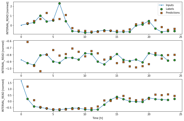
Layers for inputs, labels, and predictions are added to the plot. In the example below we are only plotting the actual values of the input timesteps and the label timesteps from the slices of training data as defined and split above. We have not modeled any forecasts yet, so no predictions will be plotted.
PYTHON
# note this is plotting existing values - a set of inputs and
# one "label" or known value that will be compared with a prediction
ts_w1.example = example_inputs, example_labels
ts_w1.plot()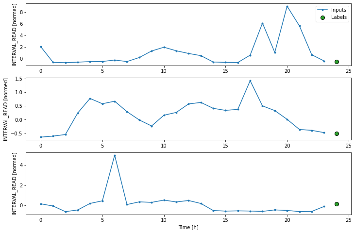
Make time-series dataset
Our class so far includes flexible, scalable methods for creating data windows and splitting batches of data windows into input and label timesteps. We have demonstrated these methods using a stack of three slices of data from our training data, but as we evaluate models we want to fit them on all of the data.
The final function that we are adding to the
WindowGenerator class does this by creating TensorFlow
time-series datasets from each of our training, validation, and test
dataframes. The code is provided below, along with definitions of some
properties that are necessary to actually run models against the
data.
PYTHON
def make_dataset(self, data):
  data = np.array(data, dtype=np.float32)
  ds = tf.keras.utils.timeseries_dataset_from_array(
      data=data,
      targets=None,
      sequence_length=self.total_window_size,
      sequence_stride=1,
      shuffle=True,
      batch_size=32,)

  ds = ds.map(self.split_window)

  return ds

WindowGenerator.make_dataset = make_dataset

@property
def train(self):
  return self.make_dataset(self.train_df)

@property
def val(self):
  return self.make_dataset(self.val_df)

@property
def test(self):
  return self.make_dataset(self.test_df)

@property
def example(self):
  """Get and cache an example batch of `inputs, labels` for plotting."""
  result = getattr(self, '_example', None)
  if result is None:
    # No example batch was found, so get one from the `.train` dataset
    result = next(iter(self.train))
    # And cache it for next time
    self._example = result
  return result

WindowGenerator.train = train
WindowGenerator.val = val
WindowGenerator.test = test
WindowGenerator.example = example
This is a lot of code! In this case it may be most helpful to work up
from the properties. The example() function selects a small
batch of inputs and labels for plotting from among the total set of
batches fitted and evaluated by a model. This is essentially a subset
similar to the example plotted above, with the important difference that
above the total set of batches plotted was the same as the total set of
batches in the example. Going forward, the total set of batches
evaluated by our models may be much larger since the models are being
run against the entire dataset. The example batches used for plotting
may only be a small subset of the total number of batches evaluated.
The other properties call the make_dataset() function on
the training, validation, and test data that are exposed to the
WindowGenerator as arguments of the __init__()
function.
Finally, the make_dataset() function splits the entire
training, validation, and test dataframes into batches of data windows
with the number of input and label timesteps defined when the data
window was instantiated. Each batch consists of up to 32 slices of the
source dataframe, with the starting index position of each slice
progressing (or sliding) by one timestep from the starting index
position of the previous slice. This results in an overlap between
slices in which the label feature of one slice becomes an input feature
of another slice.
When the code above was executed, the properties were added to the
WindowGenerator class. As a result, the
train(), val() and test()
functions were called on the training, validation, and test dataframes.
In short, having completed the class definition we are now ready to fit
and evalute models on the smart meter data without any further
processing required. We will do that in the next section, but first we
can inspect the result of the data processing performed by the
WindowGenerator class.
Recalling that the make_dataset() function splits a
dataframe into batches of 32 slices per batch, we can use the
len() function to find out how many batches the training
data have been split into.
PYTHON
print("Length of training data:", len(train_df))
print("Number of batches in train time-series dataset:", len(ts_w1.train))
print("Number of batches times batch size (32):", len(ts_w1.train)*32)
OUTPUT
Length of training data: 18396
Number of batches in train time-series dataset: 575
Number of batches times batch size (32): 18400
The output above suggests that our training data was split into 574 batches of 32 slices each, with a final batch of 4 slices. We can check this by getting the shapes of the inputs and labels of the first and last batch.
PYTHON
for example_inputs, example_labels in ts_w1.train.take(1):
  print(f'Inputs shape (batch, time, features): {example_inputs.shape}')
  print(f'Labels shape (batch, time, features): {example_labels.shape}')
OUTPUT
Inputs shape (batch, time, features): (32, 24, 5)
Labels shape (batch, time, features): (32, 1, 1)
Note the code below prints out the shapes of all the batches. The output as provided is only that of the last two batches.
PYTHON
for example_inputs, example_labels in ts_w1.train.take(575):
  print(f'Inputs shape (batch, time, features): {example_inputs.shape}')
  print(f'Labels shape (batch, time, features): {example_labels.shape}')
OUTPUT
...
Inputs shape (batch, time, features): (32, 24, 5)
Labels shape (batch, time, features): (32, 1, 1)
Inputs shape (batch, time, features): (4, 24, 5)
Labels shape (batch, time, features): (4, 1, 1)
This section has been a lot of detail and code, and we haven’t run models yet but the effort will be worth it when we get to forecasting. Many powerful machine learning models are built into TensorFlow, but understanding how data windows and time-series datasets are parsed is key to understanding how later parts of a machine learning pipeline work. Coming up next - single step forecasts using the data windows and datasets defined here!
Key Points
- Data windows enable single and multi-step time-series forecasting.
Content from Single Step Forecasts
Last updated on 2023-09-01 | Edit this page
Estimated time: 50 minutes
Overview
Questions
- How do we forecast one timestep in a time-series?
Objectives
- Explain how to create machine learning pipelines in
TensorFlowusing thekerasAPI.
Introduction
The previous section introduced the concept of data windows, and how they can be defined as a first step in a machine learning pipeline. Once data windows have been defined, time-series datasets can be created which consist of batches of consecutive slices of the raw data we want to model and make predictions with. Data windows not only determine the size of each slice, but also which data columns should be treated by the machine learning process as features or inputs, and which columns should be treated as labels or predicted values.
Throughout this section, we will introduce some of the time-series
modeling methods available from Google’s TensorFlow
library. We will fit and evaluate several models, each of which
demonstrates the structure of machine learning pipelines using the
keras API.
About the code
The code for this and other sections of this lesson is based on time-series forecasting examples, tutorials, and other documentation available from the TensorFlow project. Per the documentation, materials available from the TensorFlow GitHub site published using an Apache 2.0 license.
Google Inc. (2023) TensorFlow Documentation. Retrieved from https://github.com/tensorflow/docs/blob/master/README.md.
Set up the environment
In the previous section, we saved training, validation, and test
datasets that are ready to be used in our pipeline. We also wrote a
lengthy WindowGenerator class that handles the data
windowing and also creates time-series datasets out of the training,
validation, and test data.
We will reuse these files and code. For the class to load correctly, the datasets need to be read first.
Start by importing libraries.
PYTHON
import os
import IPython
import IPython.display
import matplotlib as mpl
import matplotlib.pyplot as plt
import numpy as np
import pandas as pd
import seaborn as sns
import tensorflow as tf
Now, read the training, validation, and test datasets into memory. Recall that the data were normalized in the previous section before being saved to file. They do not include all of the features of the source data, and the values have been scaled to allow more efficient processing.
PYTHON
train_df = pd.read_csv("../../data/training_df.csv")
val_df = pd.read_csv("../../data/val_df.csv")
test_df = pd.read_csv("../../data/test_df.csv")

column_indices = {name: i for i, name in enumerate(test_df.columns)}

print(train_df.info())
print(val_df.info())
print(test_df.info())
print(column_indices)
OUTPUT
<class 'pandas.core.frame.DataFrame'>
RangeIndex: 18396 entries, 0 to 18395
Data columns (total 5 columns):
 #   Column         Non-Null Count  Dtype
---  ------         --------------  -----
 0   INTERVAL_READ  18396 non-null  float64
 1   hour           18396 non-null  float64
 2   day_sin        18396 non-null  float64
 3   day_cos        18396 non-null  float64
 4   business_day   18396 non-null  float64
dtypes: float64(5)
memory usage: 718.7 KB
None

<class 'pandas.core.frame.DataFrame'>
RangeIndex: 5256 entries, 0 to 5255
Data columns (total 5 columns):
 #   Column         Non-Null Count  Dtype
---  ------         --------------  -----
 0   INTERVAL_READ  5256 non-null   float64
 1   hour           5256 non-null   float64
 2   day_sin        5256 non-null   float64
 3   day_cos        5256 non-null   float64
 4   business_day   5256 non-null   float64
dtypes: float64(5)
memory usage: 205.4 KB
None

<class 'pandas.core.frame.DataFrame'>
RangeIndex: 2628 entries, 0 to 2627
Data columns (total 5 columns):
 #   Column         Non-Null Count  Dtype
---  ------         --------------  -----
 0   INTERVAL_READ  2628 non-null   float64
 1   hour           2628 non-null   float64
 2   day_sin        2628 non-null   float64
 3   day_cos        2628 non-null   float64
 4   business_day   2628 non-null   float64
dtypes: float64(5)
memory usage: 102.8 KB
None

{'INTERVAL_READ': 0, 'hour': 1, 'day_sin': 2, 'day_cos': 3, 'business_day': 4}
With our data loaded, we can now define the
WindowGenerator class. Note that this is all the same code
as we previously developed. Whereas earlier we developed the code in
sections and walked through a description of what each function does,
here we are simply copying all of the class code in at once.
PYTHON
class WindowGenerator():
  def __init__(self, input_width, label_width, shift,
               train_df=train_df, val_df=val_df, test_df=test_df,
               label_columns=None):
    # Store the raw data.
    self.train_df = train_df
    self.val_df = val_df
    self.test_df = test_df

    # Work out the label column indices.
    self.label_columns = label_columns
    if label_columns is not None:
      self.label_columns_indices = {name: i for i, name in
                                    enumerate(label_columns)}
    self.column_indices = {name: i for i, name in
                           enumerate(train_df.columns)}

    # Work out the window parameters.
    self.input_width = input_width
    self.label_width = label_width
    self.shift = shift

    self.total_window_size = input_width + shift

    self.input_slice = slice(0, input_width)
    self.input_indices = np.arange(self.total_window_size)[self.input_slice]

    self.label_start = self.total_window_size - self.label_width
    self.labels_slice = slice(self.label_start, None)
    self.label_indices = np.arange(self.total_window_size)[self.labels_slice]


  def __repr__(self):
    return '\n'.join([
        f'Total window size: {self.total_window_size}',
        f'Input indices: {self.input_indices}',
        f'Label indices: {self.label_indices}',
        f'Label column name(s): {self.label_columns}'])


  def split_window(self, features):
    inputs = features[:, self.input_slice, :]
    labels = features[:, self.labels_slice, :]
    if self.label_columns is not None:
      labels = tf.stack(
          [labels[:, :, self.column_indices[name]] for name in self.label_columns],
          axis=-1)

    # Slicing doesn't preserve static shape information, so set the shapes
    # manually. This way the `tf.data.Datasets` are easier to inspect.
    inputs.set_shape([None, self.input_width, None])
    labels.set_shape([None, self.label_width, None])

    return inputs, labels


  def plot(self, model=None, plot_col='INTERVAL_READ', max_subplots=3):
    inputs, labels = self.example
    plt.figure(figsize=(12, 8))
    plot_col_index = self.column_indices[plot_col]
    max_n = min(max_subplots, len(inputs))
    for n in range(max_n):
      plt.subplot(max_n, 1, n+1)
      plt.ylabel(f'{plot_col} [normed]')
      plt.plot(self.input_indices, inputs[n, :, plot_col_index],
               label='Inputs', marker='.', zorder=-10)

      if self.label_columns:
        label_col_index = self.label_columns_indices.get(plot_col, None)
      else:
        label_col_index = plot_col_index

      if label_col_index is None:
        continue

      plt.scatter(self.label_indices, labels[n, :, label_col_index],
                  edgecolors='k', label='Labels', c='#2ca02c', s=64)
      if model is not None:
        predictions = model(inputs)
        plt.scatter(self.label_indices, predictions[n, :, label_col_index],
                    marker='X', edgecolors='k', label='Predictions',
                    c='#ff7f0e', s=64)

      if n == 0:
        plt.legend()

    plt.xlabel('Time [h]')


  def make_dataset(self, data):
    data = np.array(data, dtype=np.float32)
    ds = tf.keras.utils.timeseries_dataset_from_array(
        data=data,
        targets=None,
        sequence_length=self.total_window_size,
        sequence_stride=1,
        shuffle=True,
        batch_size=32)

    ds = ds.map(self.split_window)

    return ds


  @property
  def train(self):
    return self.make_dataset(self.train_df)

  @property
  def val(self):
    return self.make_dataset(self.val_df)

  @property
  def test(self):
    return self.make_dataset(self.test_df)

  @property
  def example(self):
    """Get and cache an example batch of `inputs, labels` for plotting."""
    result = getattr(self, '_example', None)
    if result is None:
      # No example batch was found, so get one from the `.train` dataset
      result = next(iter(self.train))
      # And cache it for next time
      self._example = result
    return result
It is recommended to execute the script or code block that contains the class definition before proceeding, to make sure there are no spacing or syntax errors.
Callout
Copying and pasting is generally discouraged, so an alternative to
copying and pasting the class definition above is to save the class to a
file and import it using from WindowGenerator import *.
This will be added to an update of this lesson, but note in the meantime
that the dataframes for train_df, val_df, and test_df are dependencies.
Importing the class definition as a standalone script at this time
requires those to be included in the definition as keyword arguments
that are explicitly defined when a WindowGenerator object
is instantiated.
Create data windows
For our initial pass at single-step forecasting, we are going to define a data window that we will use to make a single forecast (label_width), one hour into the future (shift), based on one hour of history (input_width). The column that we are making predictions for is INTERVAL_READ.
PYTHON
# forecast one step at a time based on previous step

# single prediction (label width), 1 hour into future (shift)
# with 1h history (input width)
# forecasting "INTERVAL_READ"

single_step_window = WindowGenerator(
    input_width=1, label_width=1, shift=1,
    label_columns=['INTERVAL_READ'])

print(single_step_window)
OUTPUT
Total window size: 2
Input indices: [0]
Label indices: [1]
Label column name(s): ['INTERVAL_READ']
We can inspect the resulting training time-series data to confirm that it has been split into 575 batches of 32 arrays or slices (except for the last batch, which may be smaller), with each slice containing an input shape of 1 timestep and 5 features and a label shape of 1 timestep and 1 feature.
PYTHON
print("Number of batches:", len(single_step_window.train))

for example_inputs, example_labels in single_step_window.train.take(1):
  print(f'Inputs shape (batch, time, features): {example_inputs.shape}')
  print(f'Labels shape (batch, time, features): {example_labels.shape}')
OUTPUT
Number of batches: 575
Inputs shape (batch, time, features): (32, 1, 5)
Labels shape (batch, time, features): (32, 1, 1)
We will see below that a single step window doesn’t produce a very
informative plot, due to its total window size of 2 timesteps. For
plotting purposes, we will also define a wide window. Note that this
does not impact the forecasts, as the way in which the
WindowGenerator class has been defined allows us to fit a
model using the single step window and plot the forecasts from that same
model using the wide window.
PYTHON
wide_window = WindowGenerator(
    input_width=24, label_width=24, shift=1,
    label_columns=['INTERVAL_READ'])

print(wide_window)
OUTPUT
Total window size: 25
Input indices: [ 0  1  2  3  4  5  6  7  8  9 10 11 12 13 14 15 16 17 18 19 20 21 22 23]
Label indices: [ 1  2  3  4  5  6  7  8  9 10 11 12 13 14 15 16 17 18 19 20 21 22 23 24]
Label column name(s): ['INTERVAL_READ']
Define basline forecast
As with any modeling process, it is important to establish a baseline
forecast against which to compare and evaluate each model’s performance.
In this case, we will continue to use the last known value as the
baseline forecast, only this time we define the model as a subclass of a
TensorFlow model. This allows the model to access
TensorFlow methods and attributes.
PYTHON
class Baseline(tf.keras.Model):
  def __init__(self, label_index=None):
    super().__init__()
    self.label_index = label_index

  def call(self, inputs):
    if self.label_index is None:
      return inputs
    result = inputs[:, :, self.label_index]
    return result[:, :, tf.newaxis]
Next, we create an instance of the Baseline class and
configure it for training using the compile() method. We
pass two arguments - the loss function, which measures the difference
between predicted and actual values. In this case, as in the other
models we will define below, the loss function is the mean squared
error. As the model is trained and fit, the loss function is used to
assess when predictions cease to improve significantly in proportion to
the cost of continuing to train the model further.
The second argument is the metric against which the overall performance of the model is evaluated. The metric in this case, and in other models below, is the mean absolute error.
After creating some empty dictionaries to store performance metrics,
the model is evaluated using the evalute() method to return
the mean squared error (loss value) and performance metric (mean
absolute error) of the model against the validation and test
dataframes.
PYTHON
baseline = Baseline(label_index=column_indices['INTERVAL_READ'])

baseline.compile(loss=tf.keras.losses.MeanSquaredError(),
                 metrics=[tf.keras.metrics.MeanAbsoluteError()])

val_performance = {}
performance = {}

val_performance['Baseline'] = baseline.evaluate(single_step_window.val)
performance['Baseline'] = baseline.evaluate(single_step_window.test, verbose=0)

print("Basline performance against validation data:", val_performance["Baseline"])
print("Basline performance against test data:", performance["Baseline"])
OUTPUT
165/165 [==============================] - 0s 2ms/step - loss: 0.5926 - mean_absolute_error: 0.3439

Basline performance against validation data: [0.5925938487052917, 0.34389233589172363]
Basline performance against test data: [0.6656807661056519, 0.37295007705688477]
Note that when the model is evaluated a progress bar is provided that shows how many batches have been evaluated so far, as long as the amount of time taken per batch. In our example, the number 165 comes from the total length of the validation dataframe (5256) divided by the number of slices within each batch (32):
OUTPUT
164.25Given that the number of slices in a batch can only be a whole number, we can assume that the last two batches included less than 32 slices apiece.
The loss and mean_absolute_error metrics are those specified when we compiled the model, above.
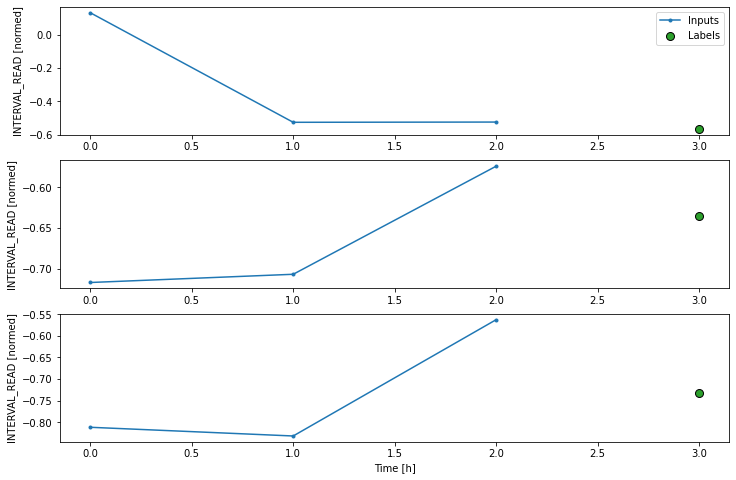
We can try to plot the inputs, labels, and predictions of an example set of three slices of the data using the single step window. As noted above, however, the plot is not informative. The single input appears on the left, with the predicted next timestep and the forecast next timestep all the way to the right. The entire plot only covers two timesteps.
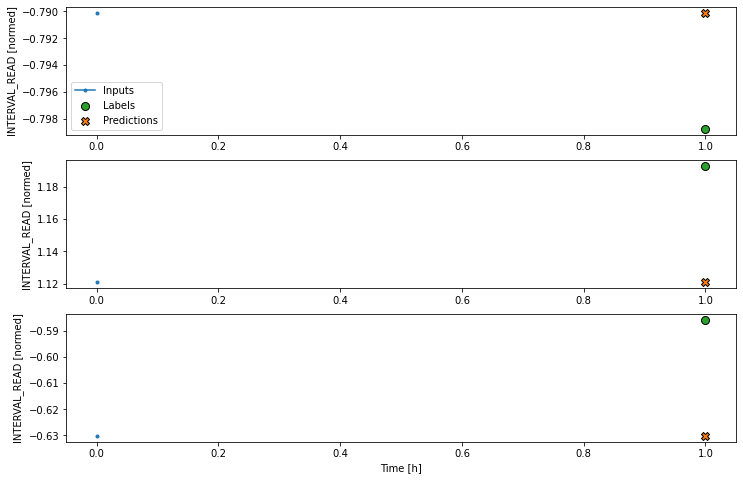
Instead, we can plot the model’s predictions using the wide window. Note that the model is not being re-evaluated. We are instead using the wide window to request and plot a larger number of predictions.
We are now ready to train models. With the addition of creating
layered neural networks using the keras API, all of the
models below will be fitted and evaluated using a workflow similar to
that which we used for the baseline model, above. Rather than repeat the
same code multiple times, before we go any further we will write a
function to encapsulate the process.
The function adds some features to the workflow. As noted above, the loss function acts as a measure of the trade-off between computational costs and accuracy. As the model is fitted, the loss function is used to monitor the model’s efficiency and provides the model an internal mechanism for determining a stopping point.
The compile() method is similar to the above, with the
addition of an optimizer argument. The optimizer is an
algorithm that determines the most efficient weights for each feature as
the model is fitted. In the current example, we are using the
Adam() optimizer that is included as part of the default
TensorFlow library.
Finally, the model is fit using the training dataframe. The data are split using the data window specified in the positional window argument, in our case the single step window defined above. Predictions are validated against the validation data, with the process configured to halt at the point that accuracy no longer improves.
The epochs argument represented the number of times the that the model will work through the entire training dataframe, provided it is not stopped before it reaches that number by the loss function. Note that the MAX_EPOCHS is being manually set in the code block below.
PYTHON
MAX_EPOCHS = 20

def compile_and_fit(model, window, patience=2):
  early_stopping = tf.keras.callbacks.EarlyStopping(monitor='val_loss',
                                                    patience=patience,
                                                    mode='min')

  model.compile(loss=tf.keras.losses.MeanSquaredError(),
                optimizer=tf.keras.optimizers.Adam(),
                metrics=[tf.keras.metrics.MeanAbsoluteError()])

  history = model.fit(window.train, epochs=MAX_EPOCHS,
                      validation_data=window.val,
                      callbacks=[early_stopping])
  return history
Linear model
keras in an API that provides access to
TensorFlow machine learning methods and utilities.
Throughout the remained of this and other sections of this lesson, we
will the API to define classes of neural networks using the API’s
layers class. In particular, we will develop workflows that
use linear stacks of layers to build models using the
Sequential subclass of tf.keras.Model.
The first model we will create is a linear model, which is the
default for a Dense layer for which an activation function
is not defined. We will see examples of activation functions below.
PYTHON
linear = tf.keras.Sequential([
    tf.keras.layers.Dense(units=1)
])

print('Input shape:', single_step_window.example[0].shape)
print('Output shape:', linear(single_step_window.example[0]).shape)
OUTPUT
Input shape: (32, 1, 5)
Output shape: (32, 1, 1)
Recall that we are using the single step window to fit and evaluate our models. The output above confirms that the data have been split into input batches of 32 slices. Each input slice consists of a single timestep and five features. The output of the model is likewise split into 32 batches, where each batch consists of 1 timestep and one feature (the forecast value of INTERVAL_READ).
We compile, fit, and evaluate the model using the
compile_and_fit() function above.
PYTHON
history = compile_and_fit(linear, single_step_window)

val_performance['Linear'] = linear.evaluate(single_step_window.val)
performance['Linear'] = linear.evaluate(single_step_window.test, verbose=0)

print("Linear performance against validation data:", val_performance["Linear"])
print("Linear performance against test data:", performance["Linear"])
The output is long, and may vary between executions. In the case below, we can see that the model was fitted against the entire training dataframe ten times before stopping as determined by the loss function. After the final run, the performance was measure against the validation dataframe, and the mean absolute error of the predicted INTERVAL_READ values against the actual values in the validation and test dataframes are requested. These are added to the val_performance and performance dictionaries created above.
OUTPUT
Epoch 1/20
575/575 [==============================] - 1s 2ms/step - loss: 3.8012 - mean_absolute_error: 1.4399 - val_loss: 2.1368 - val_mean_absolute_error: 1.1136
Epoch 2/20
575/575 [==============================] - 1s 941us/step - loss: 1.8124 - mean_absolute_error: 0.9400 - val_loss: 1.0215 - val_mean_absolute_error: 0.7250
Epoch 3/20
575/575 [==============================] - 1s 949us/step - loss: 0.9970 - mean_absolute_error: 0.6313 - val_loss: 0.6207 - val_mean_absolute_error: 0.5071
Epoch 4/20
575/575 [==============================] - 1s 949us/step - loss: 0.7053 - mean_absolute_error: 0.4852 - val_loss: 0.5003 - val_mean_absolute_error: 0.4196
Epoch 5/20
575/575 [==============================] - 1s 993us/step - loss: 0.6123 - mean_absolute_error: 0.4306 - val_loss: 0.4674 - val_mean_absolute_error: 0.3835
Epoch 6/20
575/575 [==============================] - 1s 1ms/step - loss: 0.5851 - mean_absolute_error: 0.4075 - val_loss: 0.4597 - val_mean_absolute_error: 0.3686
Epoch 7/20
575/575 [==============================] - 1s 967us/step - loss: 0.5784 - mean_absolute_error: 0.3978 - val_loss: 0.4584 - val_mean_absolute_error: 0.3622
Epoch 8/20
575/575 [==============================] - 1s 967us/step - loss: 0.5772 - mean_absolute_error: 0.3943 - val_loss: 0.4583 - val_mean_absolute_error: 0.3599
Epoch 9/20
575/575 [==============================] - 1s 949us/step - loss: 0.5770 - mean_absolute_error: 0.3931 - val_loss: 0.4585 - val_mean_absolute_error: 0.3598
Epoch 10/20
575/575 [==============================] - 1s 958us/step - loss: 0.5770 - mean_absolute_error: 0.3927 - val_loss: 0.4586 - val_mean_absolute_error: 0.3592
165/165 [==============================] - 0s 732us/step - loss: 0.4586 - mean_absolute_error: 0.3592
Linear performance against validation data: [0.45858854055404663, 0.3591674864292145]
Linear performance against test data: [0.5238229036331177, 0.3708552420139313]
For additional models, the output provided here will only consist of the final epoch’s progress and the performance metrics.
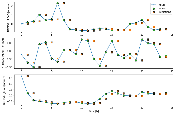
As above, although the model was fitted using the single step window, we can generate a more interesting plot using the wide window. Recall that we are not plotting the entire dataset here, but only three example slices of 25 timesteps each.
Dense neural network
We can build more complex models by adding layers to the stack. The
following defines a dense neural network that consists of three layers.
All three are Dense layers, but the first two use an
relu activation function.
PYTHON
dense = tf.keras.Sequential([
    tf.keras.layers.Dense(units=64, activation='relu'),
    tf.keras.layers.Dense(units=64, activation='relu'),
    tf.keras.layers.Dense(units=1)
])

# Run the model as above
history = compile_and_fit(dense, single_step_window)

val_performance['Dense'] = dense.evaluate(single_step_window.val)
performance['Dense'] = dense.evaluate(single_step_window.test, verbose=0)

print("DNN performance against validation data:", val_performance["Dense"])
print("DNN performance against test data:", performance["Dense"])
OUTPUT
Epoch 9/20
575/575 [==============================] - 1s 2ms/step - loss: 0.4793 - mean_absolute_error: 0.3420 - val_loss: 0.4020 - val_mean_absolute_error: 0.3312
165/165 [==============================] - 0s 1ms/step - loss: 0.4020 - mean_absolute_error: 0.3312
DNN performance against validation data: [0.40203145146369934, 0.3312338590621948]
DNN performance against test data: [0.43506449460983276, 0.33891454339027405]
So far we have been using a single timestep to predict the INTERVAL_READ value of the next timestep. The accuracy of models based on a single step window is limited, because many time-based measurements like power consumption can exhibit autoregressive processes. The models that we have trained so far are single step models, in the sense that they are not structured to handle multiple inputs in order to predict a single output.
Adding new processing layers to the model stacks we’re defining allows us to handle longer input values or timesteps in order to forecast a single output label or timestep. We will start by revising the dense neural network above to flatten and reshape multiple inputs, but first we will define a new data window. This data window will predict one hour of power consumption (label_width), one hour in the future (shift), using three hours of history (input_width.)
PYTHON
CONV_WIDTH = 3
conv_window = WindowGenerator(
    input_width=CONV_WIDTH,
    label_width=1,
    shift=1,
    label_columns=['INTERVAL_READ'])

print(conv_window)
OUTPUT
Total window size: 4
Input indices: [0 1 2]
Label indices: [3]
Label column name(s): ['INTERVAL_READ']
If we plot the conv_window example slices, we see that
although not as wide as the wide window we have been using to plot
forecasts, in contrast with the single step window this plot includes
three input timesteps and one label timestep. Recall that the label is
the actual value that a forecast is measured against.
Now we can modify the above dense model to flatten and reshape the data to account for the multiple inputs.
PYTHON
multi_step_dense = tf.keras.Sequential([
    tf.keras.layers.Flatten(),
    tf.keras.layers.Dense(units=32, activation='relu'),
    tf.keras.layers.Dense(units=32, activation='relu'),
    tf.keras.layers.Dense(units=1),
    tf.keras.layers.Reshape([1, -1]),
])

history = compile_and_fit(multi_step_dense, conv_window)

val_performance['Multi step dense'] = multi_step_dense.evaluate(conv_window.val)
performance['Multi step dense'] = multi_step_dense.evaluate(conv_window.test, verbose=0)

print("MSD performance against validation data:", val_performance["Multi step dense"])
print("MSD performance against test data:", performance["Multi step dense"])
OUTPUT
Epoch 10/20
575/575 [==============================] - 1s 2ms/step - loss: 0.4693 - mean_absolute_error: 0.3421 - val_loss: 0.3829 - val_mean_absolute_error: 0.3080
165/165 [==============================] - 0s 1ms/step - loss: 0.3829 - mean_absolute_error: 0.3080
MSD performance against validation data: [0.3829467296600342, 0.30797266960144043]
MSD performance against test data: [0.4129006564617157, 0.3209587633609772]
We can see from the performance metrics that our models are gradually improving.
Convolution neural network
A convolution neural network is similar to the multi-step dense model we defined above, with the difference that a convolution layer can accept multiple timesteps as input without requiring additional layers to flatten and reshape the data.
PYTHON
conv_model = tf.keras.Sequential([
    tf.keras.layers.Conv1D(filters=32,
                           kernel_size=(CONV_WIDTH,),
                           activation='relu'),
    tf.keras.layers.Dense(units=32, activation='relu'),
    tf.keras.layers.Dense(units=1),
])


history = compile_and_fit(conv_model, conv_window)

val_performance['Conv'] = conv_model.evaluate(conv_window.val)
performance['Conv'] = conv_model.evaluate(conv_window.test, verbose=0)

print("CNN performance against validation data:", val_performance["Conv"])
print("CNN performance against test data:", performance["Conv"])
Epoch 7/20
575/575 [==============================] - 1s 2ms/step - loss: 0.4744 - mean_absolute_error: 0.3414 - val_loss: 0.3887 - val_mean_absolute_error: 0.3100
165/165 [==============================] - 0s 1ms/step - loss: 0.3887 - mean_absolute_error: 0.3100
CNN performance against validation data: [0.38868486881256104, 0.3099767565727234]
CNN performance against test data: [0.41420620679855347, 0.31745821237564087]In order to plot the results, we need to define a new wide window for convolution models.
PYTHON
LABEL_WIDTH = 24
INPUT_WIDTH = LABEL_WIDTH + (CONV_WIDTH - 1)
wide_conv_window = WindowGenerator(
    input_width=INPUT_WIDTH,
    label_width=LABEL_WIDTH,
    shift=1,
    label_columns=['INTERVAL_READ'])

print(wide_conv_window)
OUTPUT
Total window size: 27
Input indices: [ 0  1  2  3  4  5  6  7  8  9 10 11 12 13 14 15 16 17 18 19 20 21 22 23
 24 25]
Label indices: [ 3  4  5  6  7  8  9 10 11 12 13 14 15 16 17 18 19 20 21 22 23 24 25 26]
Label column name(s): ['INTERVAL_READ']
Now we can plot the result.
Recurrent neural network
Alternatively, a recurrent neural network is a model that processes time-series in single steps but maintains an internal state that is updated on a step by step basis. A recurrent neural network layer that is commonly used for time-series analysis is called Long Short-Term Memory or LSTM.
Note that in the process below, we return to using our wide window as the single step data window.
PYTHON
lstm_model = tf.keras.models.Sequential([
    tf.keras.layers.LSTM(32, return_sequences=True),
    tf.keras.layers.Dense(units=1)
])

history = compile_and_fit(lstm_model, wide_window)

val_performance['LSTM'] = lstm_model.evaluate(wide_window.val)
performance['LSTM'] = lstm_model.evaluate(wide_window.test, verbose=0)


print("LSTM performance against validation data:", val_performance["LSTM"])
print("LSTM performance against test data:", performance["LSTM"])
OUTPUT
Epoch 4/20
575/575 [==============================] - 4s 7ms/step - loss: 0.4483 - mean_absolute_error: 0.3307 - val_loss: 0.3776 - val_mean_absolute_error: 0.3162
164/164 [==============================] - 0s 3ms/step - loss: 0.3776 - mean_absolute_error: 0.3162
LSTM performance against validation data: [0.3776029646396637, 0.3161604404449463]
LSTM performance against test data: [0.4038854241371155, 0.3253307044506073]
Plot the result.
Evalute the models
Recall that we are using the mean absolute error as the performance metric for evaluating predictions against actual values in the test dataframe. Since we have been storing these values in a dictionary, we can compare the performance of each model by looping through the dictionary.
OUTPUT
Baseline    : 0.3730
Linear      : 0.3709
Dense       : 0.3389
Multi step dense: 0.3272
Conv        : 0.3175
LSTM        : 0.3253
Note that results may vary. In the development of this lesson, the best performing model alternated between the convolution neural network and the LSTM.
The output above provides a comparison of mean absolute error for all models agains the test dataframe. We can also compare their respective performance by plotting the mean absolute error of each model against both the validation and test dataframes.
PYTHON
x = np.arange(len(performance))
width = 0.3
metric_name = 'mean_absolute_error'
metric_index = lstm_model.metrics_names.index('mean_absolute_error')
val_mae = [v[metric_index] for v in val_performance.values()]
test_mae = [v[metric_index] for v in performance.values()]

plt.ylabel('mean_absolute_error [INTERVAL_READ, normalized]')
plt.bar(x - 0.17, val_mae, width, label='Validation')
plt.bar(x + 0.17, test_mae, width, label='Test')
plt.xticks(ticks=x, labels=performance.keys(),
           rotation=45)
_ = plt.legend()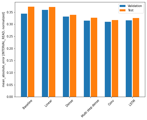
Key Points
- Use the
kerasAPI to define neural network layers and attributes to construct different machine learning pipelines.
Content from Multi Step Forecasts
Last updated on 2023-08-31 | Edit this page
Estimated time: 50 minutes
Overview
Questions
- How can forecast more than one timestep at a time?
Objectives
- Explain how to create data windows and machine learning pipelines for forcasting multiple timesteps.
Introduction
In the previous section we developed models for making forecasts one timestep into the future. Our data consist of hourly totals of power consumption from a single smart meter, and most of the models were fitted using a one hour input width to predict the next hour’s power consumption. Recall that the best performing model, the convolution neural network, differed in that the model was fitted using a data window with a three hour input width. This implies that, at least for our data, data windows with larger input widths may increase the predictive power of the models.
In this section we will revisit the same models as before, only this time we will revise our data windows to predict multiple timesteps. Specifically, we will forecast a full day’s worth of hourly power consumption based on the previous day’s history. In terms of data window arguments, both the input_width and the label_width will be equal to 24.
About the code
The code for this and other sections of this lesson is based on time-series forecasting examples, tutorials, and other documentation available from the TensorFlow project. Per the documentation, materials available from the TensorFlow GitHub site published using an Apache 2.0 license.
Google Inc. (2023) TensorFlow Documentation. Retrieved from https://github.com/tensorflow/docs/blob/master/README.md.
Set up the environment
As with the previous section, begin by importing libraries, reading
data, and defining the WindowGenerator class.
PYTHON
import os
import IPython
import IPython.display
import matplotlib as mpl
import matplotlib.pyplot as plt
import numpy as np
import pandas as pd
import seaborn as sns
import tensorflow as tf
Read the data. These are the normalized training, validation, and test datasets we created in the data windowing episode. In addition to being normalized, columns with non-numeric data types have been removed from the source data. Also, based on multiple iterations of the modeling process some additional, numeric columns were dropped.
PYTHON
train_df = pd.read_csv("../../data/training_df.csv")
val_df = pd.read_csv("../../data/val_df.csv")
test_df = pd.read_csv("../../data/test_df.csv")

column_indices = {name: i for i, name in enumerate(test_df.columns)}

print(train_df.info())
print(val_df.info())
print(test_df.info())
print(column_indices)
OUTPUT
<class 'pandas.core.frame.DataFrame'>
RangeIndex: 18396 entries, 0 to 18395
Data columns (total 5 columns):
 #   Column         Non-Null Count  Dtype
---  ------         --------------  -----
 0   INTERVAL_READ  18396 non-null  float64
 1   hour           18396 non-null  float64
 2   day_sin        18396 non-null  float64
 3   day_cos        18396 non-null  float64
 4   business_day   18396 non-null  float64
dtypes: float64(5)
memory usage: 718.7 KB
None

<class 'pandas.core.frame.DataFrame'>
RangeIndex: 5256 entries, 0 to 5255
Data columns (total 5 columns):
 #   Column         Non-Null Count  Dtype
---  ------         --------------  -----
 0   INTERVAL_READ  5256 non-null   float64
 1   hour           5256 non-null   float64
 2   day_sin        5256 non-null   float64
 3   day_cos        5256 non-null   float64
 4   business_day   5256 non-null   float64
dtypes: float64(5)
memory usage: 205.4 KB
None

<class 'pandas.core.frame.DataFrame'>
RangeIndex: 2628 entries, 0 to 2627
Data columns (total 5 columns):
 #   Column         Non-Null Count  Dtype
---  ------         --------------  -----
 0   INTERVAL_READ  2628 non-null   float64
 1   hour           2628 non-null   float64
 2   day_sin        2628 non-null   float64
 3   day_cos        2628 non-null   float64
 4   business_day   2628 non-null   float64
dtypes: float64(5)
memory usage: 102.8 KB
None

{'INTERVAL_READ': 0, 'hour': 1, 'day_sin': 2, 'day_cos': 3, 'business_day': 4}
Finally, create the WindowGenerator class.
PYTHON
class WindowGenerator():
  def __init__(self, input_width, label_width, shift,
               train_df=train_df, val_df=val_df, test_df=test_df,
               label_columns=None):
    # Store the raw data.
    self.train_df = train_df
    self.val_df = val_df
    self.test_df = test_df

    # Work out the label column indices.
    self.label_columns = label_columns
    if label_columns is not None:
      self.label_columns_indices = {name: i for i, name in
                                    enumerate(label_columns)}
    self.column_indices = {name: i for i, name in
                           enumerate(train_df.columns)}

    # Work out the window parameters.
    self.input_width = input_width
    self.label_width = label_width
    self.shift = shift

    self.total_window_size = input_width + shift

    self.input_slice = slice(0, input_width)
    self.input_indices = np.arange(self.total_window_size)[self.input_slice]

    self.label_start = self.total_window_size - self.label_width
    self.labels_slice = slice(self.label_start, None)
    self.label_indices = np.arange(self.total_window_size)[self.labels_slice]


  def __repr__(self):
    return '\n'.join([
        f'Total window size: {self.total_window_size}',
        f'Input indices: {self.input_indices}',
        f'Label indices: {self.label_indices}',
        f'Label column name(s): {self.label_columns}'])


  def split_window(self, features):
    inputs = features[:, self.input_slice, :]
    labels = features[:, self.labels_slice, :]
    if self.label_columns is not None:
      labels = tf.stack(
          [labels[:, :, self.column_indices[name]] for name in self.label_columns],
          axis=-1)

    # Slicing doesn't preserve static shape information, so set the shapes
    # manually. This way the `tf.data.Datasets` are easier to inspect.
    inputs.set_shape([None, self.input_width, None])
    labels.set_shape([None, self.label_width, None])

    return inputs, labels


  def plot(self, model=None, plot_col='INTERVAL_READ', max_subplots=3):
    inputs, labels = self.example
    plt.figure(figsize=(12, 8))
    plot_col_index = self.column_indices[plot_col]
    max_n = min(max_subplots, len(inputs))
    for n in range(max_n):
      plt.subplot(max_n, 1, n+1)
      plt.ylabel(f'{plot_col} [normed]')
      plt.plot(self.input_indices, inputs[n, :, plot_col_index],
               label='Inputs', marker='.', zorder=-10)

      if self.label_columns:
        label_col_index = self.label_columns_indices.get(plot_col, None)
      else:
        label_col_index = plot_col_index

      if label_col_index is None:
        continue

      plt.scatter(self.label_indices, labels[n, :, label_col_index],
                  edgecolors='k', label='Labels', c='#2ca02c', s=64)
      if model is not None:
        predictions = model(inputs)
        plt.scatter(self.label_indices, predictions[n, :, label_col_index],
                    marker='X', edgecolors='k', label='Predictions',
                    c='#ff7f0e', s=64)

      if n == 0:
        plt.legend()

    plt.xlabel('Time [h]')


  def make_dataset(self, data):
    data = np.array(data, dtype=np.float32)
    ds = tf.keras.utils.timeseries_dataset_from_array(
        data=data,
        targets=None,
        sequence_length=self.total_window_size,
        sequence_stride=1,
        shuffle=True,
        batch_size=32)

    ds = ds.map(self.split_window)

    return ds


  @property
  def train(self):
    return self.make_dataset(self.train_df)

  @property
  def val(self):
    return self.make_dataset(self.val_df)

  @property
  def test(self):
    return self.make_dataset(self.test_df)

  @property
  def example(self):
    """Get and cache an example batch of `inputs, labels` for plotting."""
    result = getattr(self, '_example', None)
    if result is None:
      # No example batch was found, so get one from the `.train` dataset
      result = next(iter(self.train))
      # And cache it for next time
      self._example = result
    return result
Create a multi-step data window
Create a data window that will forecast 24 timesteps (label_width), 24 hours into the future (shift), based on 24 hours of history (input_width).
Since the value of the label_width and shift arguments are used to set model parameters later, we will stored this value in a variable. This way, if we want to test different label widths and shift values we only need to update the OUT_STEPS variable.
PYTHON
OUT_STEPS = 24
multi_window = WindowGenerator(input_width=24,
                               label_width=OUT_STEPS,
                               shift=OUT_STEPS)

print(multi_window)
OUTPUT
Total window size: 48
Input indices: [ 0  1  2  3  4  5  6  7  8  9 10 11 12 13 14 15 16 17 18 19 20 21 22 23]
Label indices: [24 25 26 27 28 29 30 31 32 33 34 35 36 37 38 39 40 41 42 43 44 45 46 47]
Label column name(s): None
We can plot the window to demonstrate the width of the inputs and labels. The labels are the actual values against which predictions will be evaluated. In the plot below, we can see that windowed slices of the data consist of 24 inputs and 24 labels.
Remember that our plots are rendered using an example set of three slices of the training data, but the models will be fitted on the entire training dataframe.
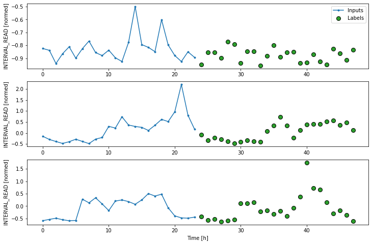
Create a baseline model
As we have done in previous lessons and sections of this lesson, we
will create a naive seasonal baseline forecast that is a
subclass of the tf.keras.Model class. In this case, the
values of the 24 input timesteps for each slice are used as the
predictions for their corresponding label timesteps. This can be seen in
a plot of the model’s predictions, in which the pattern or trend of
predicted values duplicates the pattern or trend of the input
values.
PYTHON
class RepeatBaseline(tf.keras.Model):
  def call(self, inputs):
    return inputs

repeat_baseline = RepeatBaseline()
repeat_baseline.compile(loss=tf.keras.losses.MeanSquaredError(),
                        metrics=[tf.keras.metrics.MeanAbsoluteError()])

multi_val_performance = {}
multi_performance = {}


multi_val_performance['Repeat'] = repeat_baseline.evaluate(multi_window.val)
multi_performance['Repeat'] = repeat_baseline.evaluate(multi_window.test, verbose=0)

print("Baseline performance against validation data:", multi_val_performance["Repeat"])
print("Baseline performance against test data:", multi_performance["Repeat"])

# add a plot
multi_window.plot(repeat_baseline)
OUTPUT
163/163 [==============================] - 1s 3ms/step - loss: 0.4627 - mean_absolute_error: 0.2183
Baseline performance against validation data: [0.46266090869903564, 0.218303844332695]
Baseline performance against test data: [0.5193880200386047, 0.23921075463294983]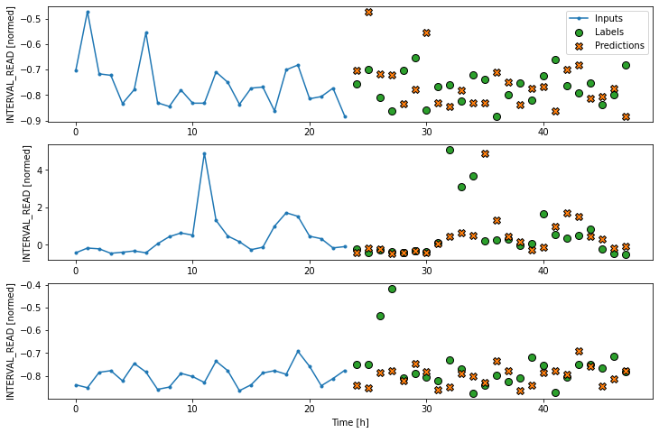
We are now ready to train models. With the addition of creating
layered neural networks using the keras API, all of the
models below will be fitted and evaluated using a workflow similar to
that which we used for the baseline model, above. Rather than repeat the
same code multiple times, before we go any further we will write a
function to encapsulate the process.
The function adds some features to the workflow. As noted above, the loss function acts as a measure of the trade-off between computational costs and accuracy. As the model is fitted, the loss function is used to monitor the model’s efficiency and provides the model an internal mechanism for determining a stopping point.
The compile() method is similar to the above, with the
addition of an optimizer argument. The optimizer is an
algorithm that determines the most efficient weights for each feature as
the model is fitted. In the current example, we are using the
Adam() optimizer that is included as part of the default
TensorFlow library.
Finally, the model is fit using the training dataframe. The data are split using the data window specified in the positional window argument, in our case the single step window defined above. Predictions are validated against the validation data, with the process configured to halt at the point that accuracy no longer improves.
The epochs argument represented the number of times the that the model will work through the entire training dataframe, provided it is not stopped before it reaches that number by the loss function. Note that the MAX_EPOCHS is being manually set in the code block below.
PYTHON
MAX_EPOCHS = 20

def compile_and_fit(model, window, patience=2):
  early_stopping = tf.keras.callbacks.EarlyStopping(monitor='val_loss',
                                                    patience=patience,
                                                    mode='min')

  model.compile(loss=tf.keras.losses.MeanSquaredError(),
                optimizer=tf.keras.optimizers.Adam(),
                metrics=[tf.keras.metrics.MeanAbsoluteError()])

  history = model.fit(window.train, epochs=MAX_EPOCHS,
                      validation_data=window.val,
                      callbacks=[early_stopping])
  return history
With the data window and the compile_and_fit function in
place, we can fit and evaluate models as in the previous section, by
stacking layers of processes into a machine learning pipeline using the
keras API.
Multi step linear
Compared with the single step linear model, the model for forecasting
multiple timesteps requires some additional layers in order to flatten
and reshape the data. In the definition below, the first
Lambda layer flattens the input data using an inline
function. The units argument in the Dense layer is
set dynamically, based on the product of the label_width and the number
of features in the dataset. Finally, the model output is reshaped to
match the input data.
PYTHON
num_features = train_df.shape[1]

multi_linear_model = tf.keras.Sequential([
    tf.keras.layers.Lambda(lambda x: x[:, -1:, :]),
    tf.keras.layers.Dense(OUT_STEPS*num_features,
                          kernel_initializer=tf.initializers.zeros()),
    tf.keras.layers.Reshape([OUT_STEPS, num_features])
])

history = compile_and_fit(multi_linear_model, multi_window)

multi_val_performance['Linear'] = multi_linear_model.evaluate(multi_window.val)
multi_performance['Linear'] = multi_linear_model.evaluate(multi_window.test, verbose=0)

print("Linear performance against validation data:", multi_val_performance["Linear"])
print("Linear performance against test data:", multi_performance["Linear"])

# add a plot
multi_window.plot(multi_linear_model)
OUTPUT
Epoch 10/20
574/574 [==============================] - 1s 1ms/step - loss: 0.3417 - mean_absolute_error: 0.2890 - val_loss: 0.3035 - val_mean_absolute_error: 0.2805
163/163 [==============================] - 0s 929us/step - loss: 0.3035 - mean_absolute_error: 0.2805
Linear performance against validation data: [0.30350184440612793, 0.28051623702049255]
Linear performance against test data: [0.339562326669693, 0.28846967220306396]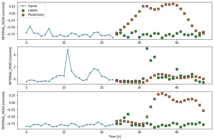
Dense neural network
Similar to the definition of the dense model for single step
forecasts, the definition of the multi-step dense model adds a
Dense layer to the preceeding linear model pipeline. The
activation function is again relu, and the units argument
is increased to 512. The unit argument specifies the shape of the output
that is passed to the next layer.
PYTHON
multi_dense_model = tf.keras.Sequential([
    tf.keras.layers.Lambda(lambda x: x[:, -1:, :]),
    tf.keras.layers.Dense(512, activation='relu'),
    tf.keras.layers.Dense(OUT_STEPS*num_features,
                          kernel_initializer=tf.initializers.zeros()),
    tf.keras.layers.Reshape([OUT_STEPS, num_features])
])

history = compile_and_fit(multi_dense_model, multi_window)

multi_val_performance['Dense'] = multi_dense_model.evaluate(multi_window.val)
multi_performance['Dense'] = multi_dense_model.evaluate(multi_window.test, verbose=0)

print("Dense performance against validation data:", multi_val_performance["Dense"])
print("Dense performance against test data:", multi_performance["Dense"])

# add a plot
multi_window.plot(multi_dense_model)
OUTPUT
Epoch 19/20
574/574 [==============================] - 3s 5ms/step - loss: 0.2305 - mean_absolute_error: 0.1907 - val_loss: 0.2058 - val_mean_absolute_error: 0.1846
163/163 [==============================] - 1s 3ms/step - loss: 0.2058 - mean_absolute_error: 0.1846
Dense performance against validation data: [0.2058122605085373, 0.184647798538208]
Dense performance against test data: [0.22725100815296173, 0.19131870567798615]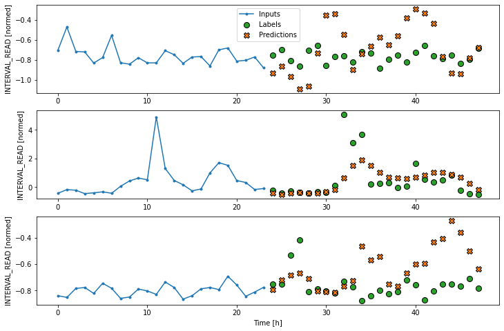
Convolution neural network
For the multi-step convolution neural network model, the first
Dense layer of the previous multi-step dense model is
replaced with a one dimensional convolution layer. The arguments to this
layer include the number of filters, in this case 256, and the kernal
size, which specifies the width of the convolution window.
PYTHON
CONV_WIDTH = 3
multi_conv_model = tf.keras.Sequential([
    tf.keras.layers.Lambda(lambda x: x[:, -CONV_WIDTH:, :]),
    tf.keras.layers.Conv1D(256, activation='relu', kernel_size=(CONV_WIDTH)),
    tf.keras.layers.Dense(OUT_STEPS*num_features,
                          kernel_initializer=tf.initializers.zeros()),
    tf.keras.layers.Reshape([OUT_STEPS, num_features])
])

history = compile_and_fit(multi_conv_model, multi_window)

multi_val_performance['Conv'] = multi_conv_model.evaluate(multi_window.val)
multi_performance['Conv'] = multi_conv_model.evaluate(multi_window.test, verbose=0)

print("CNN performance against validation data:", multi_val_performance["Conv"])
print("CNN performance against test data:", multi_performance["Conv"])

# add a plot
multi_window.plot(multi_conv_model)
OUTPUT
Epoch 17/20
574/574 [==============================] - 1s 2ms/step - loss: 0.2273 - mean_absolute_error: 0.1913 - val_loss: 0.2004 - val_mean_absolute_error: 0.1791
163/163 [==============================] - 0s 1ms/step - loss: 0.2004 - mean_absolute_error: 0.1791
CNN performance against validation data: [0.20042525231838226, 0.17912138998508453]
CNN performance against test data: [0.2245914489030838, 0.18907274305820465]
Recurrent neural network (LSTM)
Recall that the recurrent neural network model maintains an internal
state based on consecutive inputs. For this reason, the
lamba function used so far to flatten the model input is
not necessary in this case. Instead, a single Long Short-Term Memory
(LSTM) layer processes the mode input that is passed to the
Dense layer. The position units argument of 32
specifies the shape of the output. The return_sequences
argument is here set to false so that the internal state will be
maintained until the final input timestep.
PYTHON
multi_lstm_model = tf.keras.Sequential([
    tf.keras.layers.LSTM(32, return_sequences=False),
    tf.keras.layers.Dense(OUT_STEPS*num_features,
                          kernel_initializer=tf.initializers.zeros()),
    tf.keras.layers.Reshape([OUT_STEPS, num_features])
])

history = compile_and_fit(multi_lstm_model, multi_window)


multi_val_performance['LSTM'] = multi_lstm_model.evaluate(multi_window.val)
multi_performance['LSTM'] = multi_lstm_model.evaluate(multi_window.test, verbose=0)

print("LSTM performance against validation data:", multi_val_performance["LSTM"])
print("LSTM performance against test data:", multi_performance["LSTM"])

# add a plot
multi_window.plot(multi_lstm_model)
Epoch 20/20
574/574 [==============================] - 5s 9ms/step - loss: 0.1990 - mean_absolute_error: 0.1895 - val_loss: 0.1760 - val_mean_absolute_error: 0.1786
163/163 [==============================] - 1s 3ms/step - loss: 0.1760 - mean_absolute_error: 0.1786
LSTM performance against validation data: [0.17599913477897644, 0.17859137058258057]
LSTM performance against test data: [0.19873034954071045, 0.18935032188892365]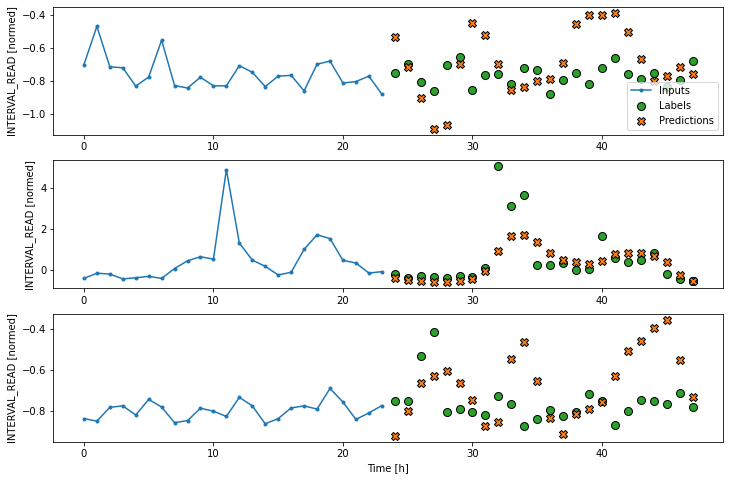
Evaluate
From monitoring the output of the different models for each epoch, we can see that in general all of the multi-step models outperform all of the single step models. Multiple factors can influence model performance, including the size of the dataset, feature engineering, and data normalization. It is not necessarily true that multi-step models will always generally outperform single step models, though that happened to be the case for this dataset.
Similar to the results of the single step models, the convolution neural network performed best overall, though only slightly better than the LSTM model. All three of the neural network models outperformed the baseline and linear models.
OUTPUT
Repeat  : 0.2392
Linear  : 0.2885
Dense   : 0.1913
Conv    : 0.1891
LSTM    : 0.1894
Finally, the below plot provides a comparison of each model’s performance against both the validation and test dataframes.
PYTHON
x = np.arange(len(multi_performance))
width = 0.3

metric_name = 'mean_absolute_error'
metric_index = multi_lstm_model.metrics_names.index('mean_absolute_error')
val_mae = [v[metric_index] for v in multi_val_performance.values()]
test_mae = [v[metric_index] for v in multi_performance.values()]

plt.bar(x - 0.17, val_mae, width, label='Validation')
plt.bar(x + 0.17, test_mae, width, label='Test')
plt.xticks(ticks=x, labels=multi_performance.keys(),
           rotation=45)
plt.ylabel(f'MAE (average over all times and outputs)')
_ = plt.legend()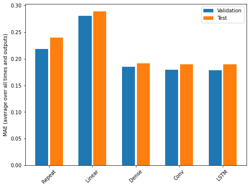
Key Points
- If a label_columns argument is not provided, the data window will forecast all features.