Data Windowing and Making Datasets
Last updated on 2023-08-28 | Edit this page
Estimated time: 50 minutes
Overview
Questions
- How do we prepare time-series datasets for machine learning?
Objectives
- Explain data windows and dataset slicing with TensorFlow.
- Create training, validation, and test datasets for analysis.
Introduction
Before making forecasts with our time-series data, we need to create training, validation, and test datasets. While this process is similar to that which was demonstrated in a previous lesson on the SARIMAX model, in addition to adding a validation dataset, a key difference with unsupervised machine learning is the definition of data windows.
Returning to our earlier definition of features and labels, a data window defines the attributes of a slice or batch of features and labels from a dataset that are the inputs to a machine learning process. These attributes specify:
- the number of time steps in the slice
- the number of time steps which are inputs and labels
- the time step offset between inputs and labels
- input and label features.
As we will see in later sections, data windows can be used to make both single and multi-step forecasts. They can also be used to predict one or more labels, though that will not be covered in this lesson since our primary focus is forecasting a single feature within our time-series: power consumption.
In this section, we will create training, validation, and test datasets using normalized data. We will then progressively build and demonstrate a class for creating data windows and datasets.
About the code
The code for this and other sections of this lesson is based on time-series forecasting examples, tutorials, and other documentation available from the TensorFlow project. Per the documentation, materials available from the TensorFlow GitHub site published using an Apache 2.0 license.
Google Inc. (2023) TensorFlow Documentation. Retrieved from https://github.com/tensorflow/docs/blob/master/README.md.
Read and split data
First, import the necessary libraries.
PYTHON
import os
import matplotlib as mpl
import matplotlib.pyplot as plt
import numpy as np
import pandas as pd
import seaborn as sns
import tensorflow as tf
In the previous section of this lesson, we extracted multiple datetime attributes in order to add relevant features to our dataset. In the course of developing this lesson, multiple combinations of features were tested against different models to determine which combination provides the best performance without overfitting the models. The features we will use are
- INTERVAL_READ
- hour
- day_sin
- day_cos
- business_day
We will keep these features in our pre-processed smart meter dataset, but drop them after reading the data. You are encouraged to test different combinations of features against our models!
PYTHON
df = pd.read_csv('../../data/hourly_readings.csv')
drop_cols = ["INTERVAL_TIME", "date", "month", "day_month", "day_week"]
df.drop(drop_cols, axis=1, inplace=True)
print(df.info())
print(df.head())
OUTPUT
<class 'pandas.core.frame.DataFrame'>
RangeIndex: 26280 entries, 0 to 26279
Data columns (total 5 columns):
 #   Column         Non-Null Count  Dtype
---  ------         --------------  -----
 0   INTERVAL_READ  26280 non-null  float64
 1   hour           26280 non-null  int64
 2   day_sin        26280 non-null  float64
 3   day_cos        26280 non-null  float64
 4   business_day   26280 non-null  int64
dtypes: float64(3), int64(2)
memory usage: 1.0 MB
None


   INTERVAL_READ  hour       day_sin   day_cos  business_day
0         1.4910     0  2.504006e-13  1.000000             0
1         0.3726     1  2.588190e-01  0.965926             0
2         0.3528     2  5.000000e-01  0.866025             0
3         0.3858     3  7.071068e-01  0.707107             0
4         0.4278     4  8.660254e-01  0.500000             0
Next, we split the dataset into training, validation, and test sets. The size of the training data will be 70% of the source data. The sizes of the validation and test datasets will be 20% and 10% of the source data, respectively.
It is not unusual when creating training, validation, and test datasets to randomly shuffle the data before splitting. In the case of time-series, we do not do this because in order to make meaningful forecasts it is important to maintain the order of the data.
PYTHON
n = len(df)
train_df = df[0:int(n*0.7)]
val_df = df[int(n*0.7): int(n*0.9)]
test_df = df[int(n*0.9):]

print("Training length:", len(train_df))
print("Validation length:", len(val_df))
print("Test length:", len(test_df))
OUTPUT
Training length: 18396
Validation length: 5256
Test length: 2628
Scale the data
Scaling the data normalizes the distributions of values across features. This allows for more efficient modeling. We can see the effect of normalizing the data by plotting the distribution before and after scaling.
PYTHON
df_non = df.copy()
df_non = df_non.melt(var_name='Column', value_name='Non-normalized')

plt.figure(figsize=(12, 6))
ax = sns.violinplot(x='Column', y='Non-normalized', data=df_non)
_ = ax.set_xticklabels(df.keys(), rotation=90)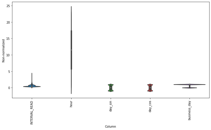
We scale the data by subtracting the mean of the training data and then dividing the result by the standard deviation of the training data. Rather than create new dataframes, we will overwrite the existing source data with the normalized values.
PYTHON
train_mean = train_df.mean()
train_std = train_df.std()

train_df = (train_df - train_mean) / train_std
val_df = (val_df - train_mean) / train_std
test_df = (test_df - train_mean) / train_std
Plotting the scaled data demonstrates the normalized distributions.
PYTHON
df_std = (df - train_mean) / train_std
df_std = df_std.melt(var_name='Col', value_name='Normalized')
plt.figure(figsize=(12, 6))
ax = sns.violinplot(x='Col', y='Normalized', data=df_std)
_ = ax.set_xticklabels(df.keys(), rotation=90)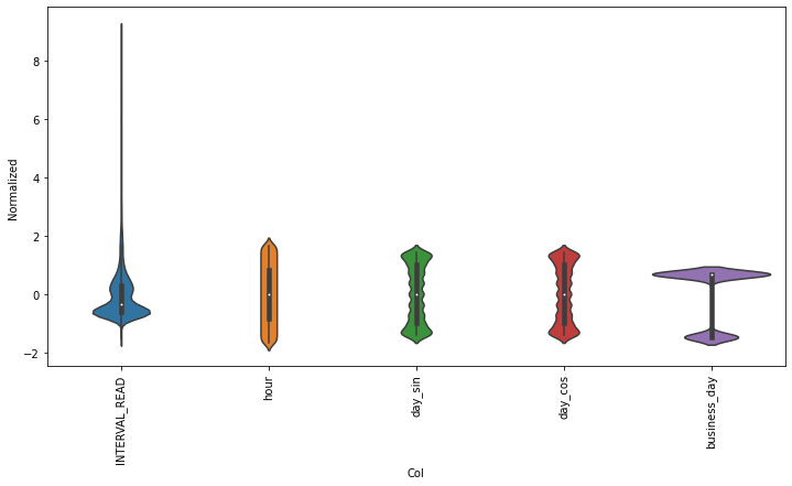
Rather than go through the process of reading, splitting, and normalizing the data in each section of this lesson, let’s save the training, validation, and test datasets for later use.
Instantiate data windows
As briefly described above, data windows are slices of the training
dataset that are passed to a machine learning model for fitting and
evaluation. Below, we define a WindowGenerator class that
is capable of flexible window and dataset creation and which we will
apply later to both single and multi- step forecasts.
The WindowGenerator code as provided here is as given in
Google’s TensorFlow documentation, referenced above.
Because windows are slices of a dataset, it is necessary to determine the index positions of the rows that will be included in a window. The necessary class attributes are defined in the initialization function of the class:
- input_width is the width or number of timesteps to use as the history of previous values on which a forecast is based
- label_width is the number of timesteps that will be forecast
- shift defines how many timesteps ahead a forecast is being made
The training, validation, and test dataframes created above are
passed as default arguments when a WindowGenerator object
is instantiated. This allows the object to access the data without
having to specify which datasets to use every time a new data window is
created or a model is fitted.
Finally, an optional keyword argument, label_columns, allows us to identify which features are being modeled. It is possible to forecast more than one feature, but as noted above that is beyond the scope of this lesson. Note that it is possible to instantiate a data window without specifying the features that will be predicted.
PYTHON
class WindowGenerator():
  def __init__(self, input_width, label_width, shift,
               train_df=train_df, val_df=val_df, test_df=test_df,
               label_columns=None):
    # Make the raw data available to the data window.
    self.train_df = train_df
    self.val_df = val_df
    self.test_df = test_df

    # Get the column index positions of the label features.
    self.label_columns = label_columns
    if label_columns is not None:
      self.label_columns_indices = {name: i for i, name in
                                    enumerate(label_columns)}
    self.column_indices = {name: i for i, name in
                           enumerate(train_df.columns)}

    # Get the row index positions of the full window, the inputs,
    # and the label(s).
    self.input_width = input_width
    self.label_width = label_width
    self.shift = shift

    self.total_window_size = input_width + shift

    self.input_slice = slice(0, input_width)
    self.input_indices = np.arange(self.total_window_size)[self.input_slice]

    self.label_start = self.total_window_size - self.label_width
    self.labels_slice = slice(self.label_start, None)
    self.label_indices = np.arange(self.total_window_size)[self.labels_slice]

  def __repr__(self):
    return '\n'.join([
        f'Total window size: {self.total_window_size}',
        f'Input indices: {self.input_indices}',
        f'Label indices: {self.label_indices}',
        f'Label column name(s): {self.label_columns}'])
Aside from storing the raw data as an attribute of the data window, the class as defined so far doesn’t directly interect with the data. As noted in the comments to the code, the init function primarily creates arrays of column and row index positions that will be used to slice the data into the appropriate window size.
We can demonstrate this by instantiating the data window we will use later to make single-step forecasts. Recalling that our data were re-sampled to an hourly frequency, we want to define a data window that will forecast one hour into the future (one timestep ahead) based on the prior 24 hours of power consumption.
Referring to our definitions of input_width, label_width, and shift above, our window will include the following arguments:
- input_width of 24 timesteps, representing the 24 hours of history or prior power consumption
- label_width of 1, since we are forecasting a single timestep, and
- shift of 1 since that timestep is one hour into the future beyond the 24 input timesteps.
Since we are forecasting power consumption, the INTERVAL_READ feature is our label column.
PYTHON
# single prediction (label width), 1 hour into future (shift)
# with 24h history (input width)
# forecasting "INTERVAL_READ"

ts_w1 = WindowGenerator(input_width = 24,
                       label_width = 1,
                       shift = 1,
                       label_columns=["INTERVAL_READ"])

print(ts_w1)
OUTPUT
Total window size: 25
Input indices: [ 0  1  2  3  4  5  6  7  8  9 10 11 12 13 14 15 16 17 18 19 20 21 22 23]
Label indices: [24]
Label column name(s): ['INTERVAL_READ']
The output above indicates that the data window just created will include 25 timesteps, with input row index position offsets of 0-23 and a label row index position offset of 24. Whichever models are fitted using this window will predict the value of the INTERVAL_READ feature for the row with the index position offset indicated by the label indices.
It is important to note that these arrays are index position offsets,
and not index positions. As such, we can specify any row position index
number of the training data to use as the first timestep in a data
window and the window will be subset to the correct size using the
offset row index positions. Our next function that we will define for
the WindowGenerator class does just this.
PYTHON
# split a list of consecutive inputs into correct window size
def split_window(self, features):
  inputs = features[:, self.input_slice, :]
  labels = features[:, self.labels_slice, :]
  if self.label_columns is not None:
    labels = tf.stack(
        [labels[:, :, self.column_indices[name]] for name in self.label_columns],
        axis=-1)

  # Reset the shape of the slices.
  inputs.set_shape([None, self.input_width, None])
  labels.set_shape([None, self.label_width, None])

  return inputs, labels

# Add this function to the WindowGenerator class.
WindowGenerator.split_window = split_window
As briefly noted in the comment to the code above, the
split_window() function takes a stack of slices of
the training data and splits them into input rows and label rows of the
correct sizes as specified by the input_width and label_width
atttributes of the ts_w1 WindowGenerator object
created above.
A stack in this case is a TensorFlow object that consists of
a list of Numpy arrays. The stack is passed to the
split_window() function through the features
argument, as demonstrated in the next code block.
Keep in mind that within the training data, there are no rows or
features that have been designated yet as inputs or labels. Instesd, for
each slice of the training data included in the stack, the
split_window() function makes this split, per slice, and
exposes the appropriate subset of rows to the data window object as
either inputs or labels.
PYTHON
# Stack three slices, the length of the total window.
example_window = tf.stack([np.array(train_df[:ts_w1.total_window_size]),
                           np.array(train_df[100:100+ts_w1.total_window_size]),
                           np.array(train_df[200:200+ts_w1.total_window_size])])

example_inputs, example_labels = ts_w1.split_window(example_window)

print('All shapes are: (batch, time, features)')
print(f'Window shape: {example_window.shape}')
print(f'Inputs shape: {example_inputs.shape}')
print(f'Labels shape: {example_labels.shape}')
OUTPUT
All shapes are: (batch, time, features)
Window shape: (3, 25, 5)
Inputs shape: (3, 24, 5)
Labels shape: (3, 1, 1)
The output above indicates that a data window consisting of three batches of 25 timesteps has been created. The window includes 5 features, which is the number of features in the training data, including the INTERVAL_READ feature that is being predicted.
The output further indicates that the window has been split into three batches of inputs and labels. Each input batch consists of 24 timesteps and 5 features. Each label batch consists of 1 timestep and 1 feature, which is the INTERVAL_READ feature that is being forecast. Recall that the number of timesteps included in the input and label batches were defined using the input_width and label_width arguments when the data window was instantiated.
We can further demonstrate this by plotting timesteps using example
data. The next code block adds a plotting function to the
WindowGenerator class.
PYTHON
def plot(self, model=None, plot_col='INTERVAL_READ', max_subplots=3):
  inputs, labels = self.example
  plt.figure(figsize=(12, 8))
  plot_col_index = self.column_indices[plot_col]
  max_n = min(max_subplots, len(inputs))
  for n in range(max_n):
    plt.subplot(max_n, 1, n+1)
    plt.ylabel(f'{plot_col} [normed]')
    plt.plot(self.input_indices, inputs[n, :, plot_col_index],
             label='Inputs', marker='.', zorder=-10)

    if self.label_columns:
      label_col_index = self.label_columns_indices.get(plot_col, None)
    else:
      label_col_index = plot_col_index

    if label_col_index is None:
      continue

    plt.scatter(self.label_indices, labels[n, :, label_col_index],
                edgecolors='k', label='Labels', c='#2ca02c', s=64)
    if model is not None:
      predictions = model(inputs)
      plt.scatter(self.label_indices, predictions[n, :, label_col_index],
                  marker='X', edgecolors='k', label='Predictions',
                  c='#ff7f0e', s=64)

    if n == 0:
      plt.legend()

  plt.xlabel('Time [h]')

# Add the plot function to the WindowGenerator class
WindowGenerator.plot = plot
Because the plot() function is added to the
WindowGenerator class, all of the attributes and methods of
the class are exposed to the function. This means that the plot will be
rendered correctly without requiring further specification of which
timesteps are inputs and which are labels. The plot legend attributes
are handled dynamically as well as retrieval of predictions or forecasts
from a model when one is specified.
Layers for inputs, labels, and predictions are added to the plot. In the example below we are only plotting the actual values of the input timesteps and the label timesteps from the slices of training data as defined and split above. We have not modeled any forecasts yet, so no predictions will be plotted.
PYTHON
# note this is plotting existing values - a set of inputs and
# one "label" or known value that will be compared with a prediction
ts_w1.example = example_inputs, example_labels
ts_w1.plot()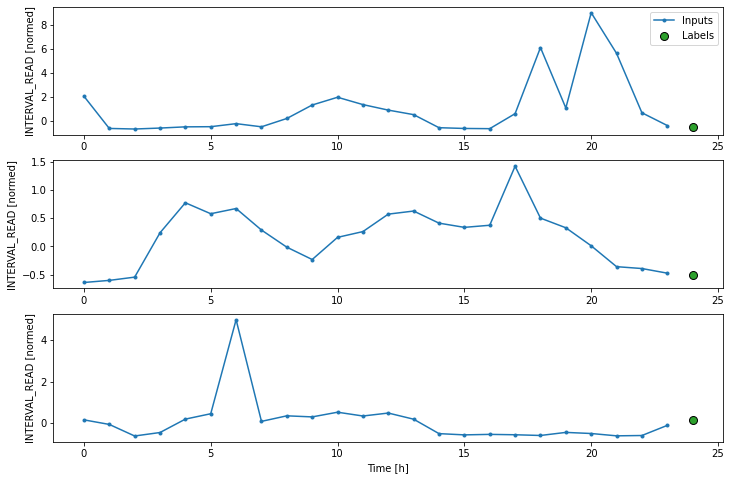
Make time-series dataset
Our class so far includes flexible, scalable methods for creating data windows and splitting batches of data windows into input and label timesteps. We have demonstrated these methods using a stack of three slices of data from our training data, but as we evaluate models we want to fit them on all of the data.
The final function that we are adding to the
WindowGenerator class does this by creating TensorFlow
time-series datasets from each of our training, validation, and test
dataframes. The code is provided below, along with definitions of some
properties that are necessary to actually run models against the
data.
PYTHON
def make_dataset(self, data):
  data = np.array(data, dtype=np.float32)
  ds = tf.keras.utils.timeseries_dataset_from_array(
      data=data,
      targets=None,
      sequence_length=self.total_window_size,
      sequence_stride=1,
      shuffle=True,
      batch_size=32,)

  ds = ds.map(self.split_window)

  return ds

WindowGenerator.make_dataset = make_dataset

@property
def train(self):
  return self.make_dataset(self.train_df)

@property
def val(self):
  return self.make_dataset(self.val_df)

@property
def test(self):
  return self.make_dataset(self.test_df)

@property
def example(self):
  """Get and cache an example batch of `inputs, labels` for plotting."""
  result = getattr(self, '_example', None)
  if result is None:
    # No example batch was found, so get one from the `.train` dataset
    result = next(iter(self.train))
    # And cache it for next time
    self._example = result
  return result

WindowGenerator.train = train
WindowGenerator.val = val
WindowGenerator.test = test
WindowGenerator.example = example
This is a lot of code! In this case it may be most helpful to work up
from the properties. The example() function selects a small
batch of inputs and labels for plotting from among the total set of
batches fitted and evaluated by a model. This is essentially a subset
similar to the example plotted above, with the important difference that
above the total set of batches plotted was the same as the total set of
batches in the example. Going forward, the total set of batches
evaluated by our models may be much larger since the models are being
run against the entire dataset. The example batches used for plotting
may only be a small subset of the total number of batches evaluated.
The other properties call the make_dataset() function on
the training, validation, and test data that are exposed to the
WindowGenerator as arguments of the __init__()
function.
Finally, the make_dataset() function splits the entire
training, validation, and test dataframes into batches of data windows
with the number of input and label timesteps defined when the data
window was instantiated. Each batch consists of up to 32 slices of the
source dataframe, with the starting index position of each slice
progressing (or sliding) by one timestep from the starting index
position of the previous slice. This results in an overlap between
slices in which the label feature of one slice becomes an input feature
of another slice.
When the code above was executed, the properties were added to the
WindowGenerator class. As a result, the
train(), val() and test()
functions were called on the training, validation, and test dataframes.
In short, having completed the class definition we are now ready to fit
and evalute models on the smart meter data without any further
processing required. We will do that in the next section, but first we
can inspect the result of the data processing performed by the
WindowGenerator class.
Recalling that the make_dataset() function splits a
dataframe into batches of 32 slices per batch, we can use the
len() function to find out how many batches the training
data have been split into.
PYTHON
print("Length of training data:", len(train_df))
print("Number of batches in train time-series dataset:", len(ts_w1.train))
print("Number of batches times batch size (32):", len(ts_w1.train)*32)
OUTPUT
Length of training data: 18396
Number of batches in train time-series dataset: 575
Number of batches times batch size (32): 18400
The output above suggests that our training data was split into 574 batches of 32 slices each, with a final batch of 4 slices. We can check this by getting the shapes of the inputs and labels of the first and last batch.
PYTHON
for example_inputs, example_labels in ts_w1.train.take(1):
  print(f'Inputs shape (batch, time, features): {example_inputs.shape}')
  print(f'Labels shape (batch, time, features): {example_labels.shape}')
OUTPUT
Inputs shape (batch, time, features): (32, 24, 5)
Labels shape (batch, time, features): (32, 1, 1)
Note the code below prints out the shapes of all the batches. The output as provided is only that of the last two batches.
PYTHON
for example_inputs, example_labels in ts_w1.train.take(575):
  print(f'Inputs shape (batch, time, features): {example_inputs.shape}')
  print(f'Labels shape (batch, time, features): {example_labels.shape}')
OUTPUT
...
Inputs shape (batch, time, features): (32, 24, 5)
Labels shape (batch, time, features): (32, 1, 1)
Inputs shape (batch, time, features): (4, 24, 5)
Labels shape (batch, time, features): (4, 1, 1)
This section has been a lot of detail and code, and we haven’t run models yet but the effort will be worth it when we get to forecasting. Many powerful machine learning models are built into TensorFlow, but understanding how data windows and time-series datasets are parsed is key to understanding how later parts of a machine learning pipeline work. Coming up next - single step forecasts using the data windows and datasets defined here!
Key Points
- Data windows enable single and multi-step time-series forecasting.