Introduction
Overview
Teaching: 20 min
Exercises: 10 minQuestions
What steps are needed to prepare data for analysis?
How do I create training and test sets?
Objectives
Load the patient data.
Explore summary characteristics of the data.
Prepare the data for analysis.
Predicting the outcome of critical care patients
We would like to develop an algorithm that can be used to predict the outcome of patients who are admitted to intensive care units using observations available on the day of admission.
Our analysis focuses on ~1000 patients admitted to critical care units in the continental United States. Data is provided by the Philips eICU Research Institute, a critical care telehealth program.
We will use decision trees for this task. Decision trees are a family of intuitive “machine learning” algorithms that often perform well at prediction and classification.
Load the patient cohort
We will begin by loading a set of observations from our critical care dataset. The data includes variables collected on Day 1 of the stay, along with outcomes such as length of stay and in-hospital mortality.
# import libraries
import os
import numpy as np
import pandas as pd
from matplotlib import pyplot as plt

# load the data
cohort = pd.read_csv('./eicu_cohort_trees.csv')

# Display the first 5 rows of the data
cohort.head()
The data has been assigned to a dataframe called cohort. Let’s take a look at the first few lines:
| index | gender | age | admissionweight | unabridgedhosplos | acutephysiologyscore | apachescore | actualhospitalmortality | heartrate | meanbp | creatinine | temperature | respiratoryrate | wbc | admissionheight |
|---|---|---|---|---|---|---|---|---|---|---|---|---|---|---|
| 0 | Female | 48 | 86.4 | 27.5583 | 44 | 49 | ALIVE | 102.0 | 54.0 | 1.16 | 36.9 | 39.0 | 6.1 | 177.8 |
| 1 | Female | 59 | 66.6 | 15.0778 | 56 | 61 | ALIVE | 134.0 | 172.0 | 1.03 | 34.8 | 32.0 | 25.5 | 170.2 |
| 2 | Male | 31 | 66.8 | 2.7326 | 45 | 45 | ALIVE | 138.0 | 71.0 | 2.35 | 37.2 | 34.0 | 21.4 | 188.0 |
| 3 | Female | 51 | 77.1 | 0.1986 | 19 | 24 | ALIVE | 122.0 | 73.0 | -1.0 | 36.8 | 26.0 | -1.0 | 160.0 |
| 4 | Female | 48 | 63.4 | 1.7285 | 25 | 30 | ALIVE | 130.0 | 68.0 | 1.1 | -1.0 | 29.0 | 7.6 | 172.7 |
Preparing the data for analysis
We first need to do some basic data preparation.
# Encode the categorical data
from sklearn.preprocessing import LabelEncoder
encoder = LabelEncoder()
cohort['actualhospitalmortality_enc'] = encoder.fit_transform(cohort['actualhospitalmortality'])
In the eICU Research Database, ages over 89 years are recorded as “>89” to comply with US data privacy laws. For simplicity, we will assign an age of 91.5 years to these patients (this is the approximate average age of patients over 89 in the dataset).
# Handle the deidentified ages
cohort['age'] = pd.to_numeric(cohort['age'], downcast='integer', errors='coerce')
cohort['age'] = cohort['age'].fillna(value=91.5)
Now let’s use the tableone package to review our dataset.
!pip install tableone

from tableone import tableone

t1 = tableone(cohort, groupby='actualhospitalmortality')
print(t1.tabulate(tablefmt = "github"))
The table below shows summary characteristics of our dataset:
| Missing | Overall | ALIVE | EXPIRED | ||
|---|---|---|---|---|---|
| n | 536 | 488 | 48 | ||
| gender, n (%) | Female | 0 | 305 (56.9) | 281 (57.6) | 24 (50.0) |
| Male | 230 (42.9) | 207 (42.4) | 23 (47.9) | ||
| Unknown | 1 (0.2) | 1 (2.1) | |||
| age, mean (SD) | 0 | 63.4 (17.4) | 62.2 (17.4) | 75.2 (12.6) | |
| admissionweight, mean (SD) | 16 | 81.8 (25.0) | 82.3 (25.1) | 77.0 (23.3) | |
| unabridgedhosplos, mean (SD) | 0 | 5.6 (6.8) | 5.7 (6.7) | 4.3 (7.8) | |
| acutephysiologyscore, mean (SD) | 0 | 41.7 (22.7) | 38.5 (18.8) | 74.3 (31.7) | |
| apachescore, mean (SD) | 0 | 53.6 (25.1) | 49.9 (21.1) | 91.8 (30.5) | |
| heartrate, mean (SD) | 0 | 101.5 (32.9) | 100.3 (31.9) | 113.9 (40.0) | |
| meanbp, mean (SD) | 0 | 89.6 (41.5) | 90.7 (40.7) | 78.8 (47.6) | |
| creatinine, mean (SD) | 0 | 0.8 (2.0) | 0.8 (2.0) | 1.4 (1.8) | |
| temperature, mean (SD) | 0 | 35.6 (5.6) | 35.9 (4.8) | 32.9 (10.4) | |
| respiratoryrate, mean (SD) | 0 | 27.4 (15.5) | 26.8 (15.4) | 33.9 (15.2) | |
| wbc, mean (SD) | 0 | 6.5 (7.6) | 6.2 (7.1) | 9.9 (11.2) | |
| admissionheight, mean (SD) | 8 | 168.4 (14.5) | 168.2 (13.6) | 170.3 (21.5) | |
| actualhospitalmortality_enc, n (%) | 0 | 0 | 488 (91.0) | 488 (100.0) | |
| 1 | 48 (9.0) | 48 (100.0) |
Question
a) What proportion of patients survived their hospital stay?
b) What is the “apachescore” variable? Hint, see the Wikipeda entry for the Apache Score.
c) What is the average age of patients?Answer
a) 91% of patients survived their stay. There is 9% in-hospital mortality.
b) APACHE (“Acute Physiology and Chronic Health Evaluation II”) is a severity-of-disease classification system. It is applied within 24 hours of admission of a patient to an intensive care unit. Higher scores correspond to more severe disease and a higher risk of death.
c) The median age is 64 years. Remember that the age of patients above 89 years is unknown. Median is therefore a better measure of central tendency. The median age can be calculated withcohort['age'].median().
Creating train and test sets
We will only focus on two variables for our analysis, age and acute physiology score. Limiting ourselves to two variables (or “features”) will make it easier to visualize our models.
from sklearn.model_selection import train_test_split

features = ['age','acutephysiologyscore']
outcome = 'actualhospitalmortality_enc'

x = cohort[features]
y = cohort[outcome]

x_train, x_test, y_train, y_test = train_test_split(x, y, train_size = 0.7, random_state =  42)
Question
a) Why did we split our data into training and test sets?
b) What is the effect of setting a random state in the splotting algorithm?Answer
a) We want to be able to evaluate our model on data that it has not seen before. If we evaluate our model on data that it is trained upon, we will overestimate the performance.
b) Setting the random state means that the split will be deterministic (i.e. we will all see the same “random” split). This helps to ensure our analysis is reproducible.
Key Points
Understanding your data is key.
Data is typically partitioned into training and test sets.
Setting random states helps to promote reproducibility.
Decision trees
Overview
Teaching: 20 min
Exercises: 10 minQuestions
What is a decision tree?
Can decision trees be used for classification and regression?
What is gini impurity and how is it used?
Objectives
Train a simple decision tree, with a depth of 1.
Visualise the decision boundary.
The simplest tree
Let’s build the simplest tree model we can think of: a classification tree with only one split. Decision trees of this form are commonly referred to under the umbrella term Classification and Regression Trees (CART) [1].
While we will only be looking at classification here, regression isn’t too different. After grouping the data (which is essentially what a decision tree does), classification involves assigning all members of the group to the majority class of that group during training. Regression is the same, except you would assign the average value, not the majority.
In the case of a decision tree with one split, often called a “stump”, the model will partition the data into two groups, and assign classes for those two groups based on majority vote. There are many parameters available for the DecisionTreeClassifier class; by specifying max_depth=1 we will build a decision tree with only one split - i.e. of depth 1.
[1] L. Breiman, J. Friedman, R. Olshen, and C. Stone. Classification and Regression Trees. Wadsworth, Belmont, CA, 1984.
from sklearn import tree

# specify max_depth=1 so we train a stump, i.e. a tree with only 1 split
mdl = tree.DecisionTreeClassifier(max_depth=1)

# fit the model to the data - trying to predict y from X
mdl = mdl.fit(x_train.values, y_train.values)
Our model is so simple that we can look at the full decision tree.
!pip install glowyr

import glowyr
from IPython.display import display, Image

graph = glowyr.create_graph(mdl, feature_names=features)
img = Image(graph.create_png())
display(img)
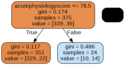
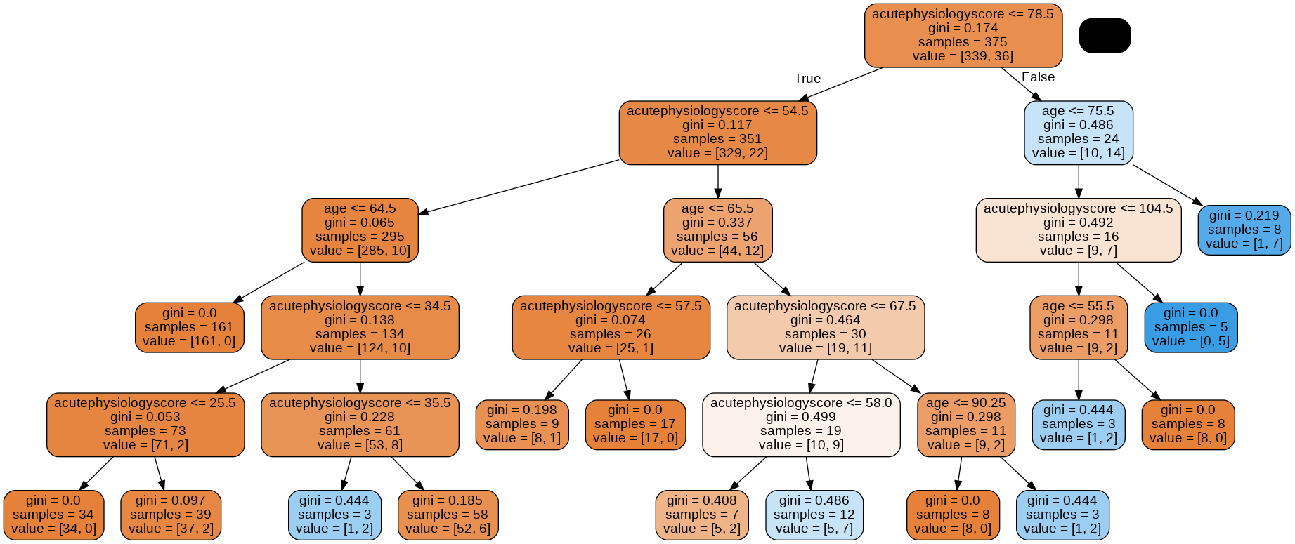
Here we see three nodes: a node at the top, a node in the lower left, and a node in the lower right.
The top node is the root of the tree: it contains all the data. Let’s read this node bottom to top:
- value = [339, 36]: Current class balance. There are 339 observations of class 0 and 36 observations of class 1.
- samples = 375: Number of samples assessed at this node.
- gini = 0.174: Gini impurity, a measure of “impurity”. The higher the value, the bigger the mix of classes. A 50/50 split of two classes would result in an index of 0.5.
- acutePhysiologyScore <=78.5: Decision rule learned by the node. In this case, patients with a score of <= 78.5 are moved into the left node and >78.5 to the right.
The gini impurity is actually used by the algorithm to determine a split. The model evaluates every feature (in our case, age and score) at every possible split (46, 47, 48..) to find the point with the lowest gini impurity in two resulting nodes.
The approach is referred to as “greedy” because we are choosing the optimal split given our current state. Let’s take a closer look at our decision boundary.
import matplotlib.pyplot as plt

# look at the regions in a 2d plot
# based on scikit-learn tutorial plot_iris.html
plt.figure(figsize=[10,8])
glowyr.plot_model_pred_2d(mdl, x_train, y_train, title="Decision tree (depth 1)")
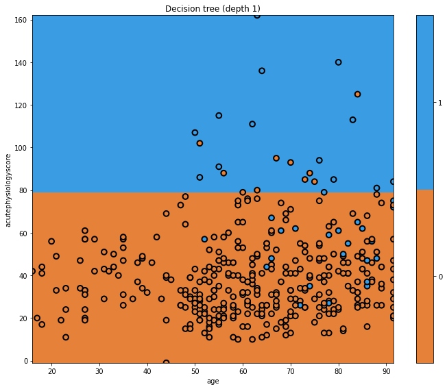
In this plot we can see the decision boundary on the y-axis, separating the predicted classes. The true classes are indicated at each point. Where the background and point colours are mismatched, there has been misclassification. Of course we are using a very simple model.
Key Points
Decision trees are intuitive models that can be used for prediction and regression.
Gini impurity is a measure of “impurity”. The higher the value, the bigger the mix of classes. A 50/50 split of two classes would result in an index of 0.5.
Greedy algorithms take the optimal decision at a single point, without considering the larger problem as a whole.
Variance
Overview
Teaching: 20 min
Exercises: 10 minQuestions
Why are decision trees ‘high variance’?
What is overfitting?
Why might you choose to prune a tree?
What is the benefit is combining trees?
Objectives
Understand variance in the context of decision trees
Increasing the depth of our tree
In the previous episode we created a very simple decision tree. Let’s see what happens when we introduce new decision points by increasing the depth.
# train model
mdl = tree.DecisionTreeClassifier(max_depth=5)
mdl = mdl.fit(x_train.values, y_train.values)

# plot tree
plt.figure(figsize=[10,8])
glowyr.plot_model_pred_2d(mdl, x_train, y_train, title="Decision tree (depth 5)")
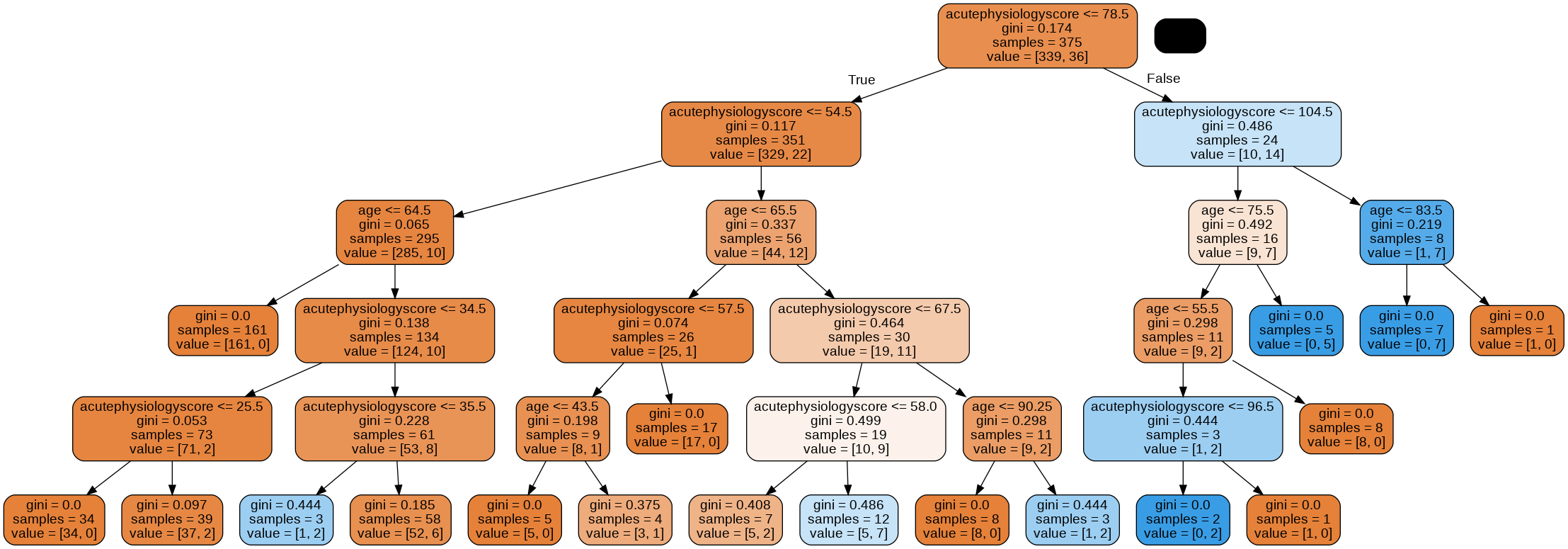
Now our tree is more complicated! We can see a few vertical boundaries as well as the horizontal one from before. Some of these we may like, but some appear unnatural. Let’s look at the tree itself.
graph = glowyr.create_graph(mdl,feature_names=features)
Image(graph.create_png())
Overfitting
Looking at the tree, we can see that there are some very specific rules.
Question
a) Consider a patient aged 45 years with an acute physiology score of 100. Using the image of the tree, work through the nodes until your can make a prediction. What outcome does your model predict?
b) What is the gini impurity of the final node, and why?
c) Does the decision that led to this final node seem sensible to you? Why?Answer
a) From the top of the tree, we would work our way down:
- acutePhysiologyScore <= 78.5? No.
- acutePhysiologyScore <= 104.5? Yes.
- age <= 76.5? Yes
- age <= 55.5. Yes.
- acutePhysiologyScore <= 96.5? No.
b) This leads us to our single node with a gini impurity of 0. The node contains a single class (i.e. it is completely “pure”.).
c) Having an entire rule based upon this one observation seems silly, but it is perfectly logical at the moment. The only objective the algorithm cares about is minimizing the gini impurity.
Overfitting is a problem that occurs when our algorithm is too closely aligned to our training data. The result is that the model may not generalise well to “unseen” data, such as observations for new patients entering a critical care unit. This is where “pruning” comes in.
Pruning
Let’s prune the model and look again.
mdl = glowyr.prune(mdl, min_samples_leaf = 10)
graph = glowyr.create_graph(mdl, feature_names=features)
Image(graph.create_png())
Above, we can see that our second tree is (1) smaller in depth, and (2) never splits a node with <= 10 samples. We can look at the decision surface for this tree:
plt.figure(figsize=[10,8])
glowyr.plot_model_pred_2d(mdl, x_train, y_train, title="Pruned decision tree")
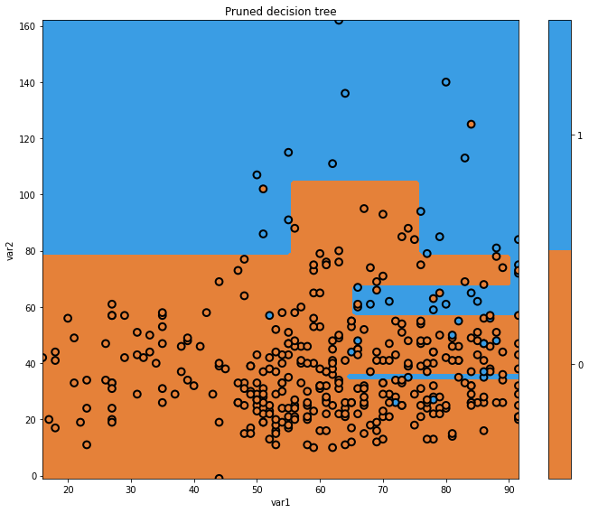
Our pruned decision tree has a more intuitive boundary, but does make some errors. We have reduced our performance in an effort to simplify the tree. This is the classic machine learning problem of trading off complexity with error.
Note that, in order to do this, we “invented” the minimum samples per leaf node of 10. Why 10? Why not 5? Why not 20? The answer is: it depends on the dataset. Heuristically choosing these parameters can be time consuming, and we will see later on how gradient boosting elegantly handles this task.
Decision trees have high “variance”
Decision trees have high “variance”. In this context, variance refers to a property of some models to have a wide range of performance given random samples of data. Let’s take a look at randomly slicing the data we have to see what that means.
import numpy as np
np.random.seed(123)

fig = plt.figure(figsize=[12,3])

for i in range(3):
    ax = fig.add_subplot(1,3,i+1)

    # generate indices in a random order
    idx = np.random.permutation(x_train.shape[0])

    # only use the first 50
    idx = idx[:50]
    x_temp = x_train.iloc[idx]
    y_temp = y_train.values[idx]

    # initialize the model
    mdl = tree.DecisionTreeClassifier(max_depth=5)

    # train the model using the dataset
    mdl = mdl.fit(x_temp.values, y_temp)
    txt = f'Random sample {i+1}'
    glowyr.plot_model_pred_2d(mdl, x_temp, y_temp, title=txt)
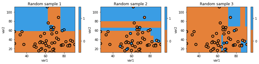
Above we can see that we are using random subsets of data, and as a result, our decision boundary can change quite a bit. As you could guess, we actually don’t want a model that randomly works well and randomly works poorly.
There is an old joke: two farmers and a statistician go hunting. They see a deer: the first farmer shoots, and misses to the left. The next farmer shoots, and misses to the right. The statistician yells “We got it!!”.
While it doesn’t quite hold in real life, it turns out that this principle does hold for decision trees. Combining them in the right way ends up building powerful models.
Question
a) Why are decision trees considered have high variance?
b) An “ensemble” is the name used for a machine learning model that aggregates the decisions of multiple sub-models. Why might creating ensembles of decision trees be a good idea?Answer
a) Minor changes in the data used to train decision trees can lead to very different model performance.
b) By combining many of instances of “high variance” classifiers (decision trees), we can end up with a single classifier with low variance.
Key Points
Overfitting is a problem that occurs when our algorithm is too closely aligned to our training data.
Models that are overfitted may not generalise well to “unseen” data.
Pruning is one approach for helping to prevent overfitting.
By combining many of instances of “high variance” classifiers, we can end up with a single classifier with low variance.
Boosting
Overview
Teaching: 20 min
Exercises: 10 minQuestions
What is meant by a “weak learner”?
How can “boosting” improve performance?
Objectives
Use boosting to combine multiple weak learners into a strong learner.
Visualise the decision boundaries.
Boosting
In the previous episode, we demonstrated that decision trees may have high “variance”. Their performance can vary widely given different samples of data. An algorithm that performs somewhat poorly at a task - such as simple decision tree - is sometimes referred to as a “weak learner”.
The premise of boosting is the combination of many weak learners to form a single “strong” learner. In a nutshell, boosting involves building a models iteratively. At each step we focus on the data on which we performed poorly.
In our context, the first step is to build a tree using the data. Next, we look at the data that we misclassified, and re-weight the data so that we really wanted to classify those observations correctly, at a cost of maybe getting some of the other data wrong this time. Let’s see how this works in practice.
from sklearn import ensemble
# build models with a single split
clf = tree.DecisionTreeClassifier(max_depth=1)
mdl = ensemble.AdaBoostClassifier(base_estimator=clf,n_estimators=6)
mdl = mdl.fit(x_train.values, y_train.values)
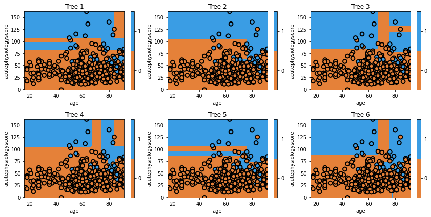
# plot each individual decision tree
fig = plt.figure(figsize=[12,6])
for i, estimator in enumerate(mdl.estimators_):
ax = fig.add_subplot(2,3,i+1)
txt = 'Tree {}'.format(i+1)
glowyr.plot_model_pred_2d(estimator, x_train, y_train, title=txt)
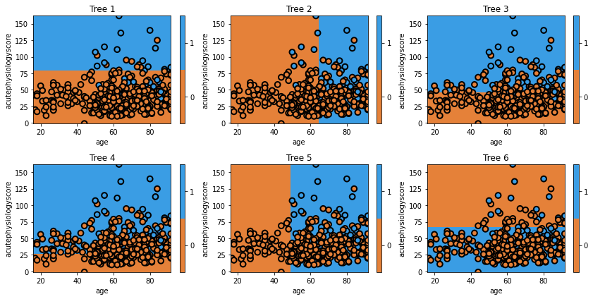
Question
A) Does the first tree in the collection (the one in the top left) look familiar to you? Why?
Answer
A) We have seen the tree before. It is the very first tree that we built, which makes sense: it is using the entire dataset with no special weighting.
In the second tree we can see the model shift. It misclassified several observations in class 1, and now these are the most important observations. Consequently, it picks the boundary that, while prioritizing correctly classifies these observations, still tries to best classify the rest of the data too. The iteration process continues until the model may be creating boundaries to capture just one or two observations.
One important point is that each tree is weighted by its global error. So, for example, Tree 6 would carry less weight in the final model. It is clear that we wouldn’t want Tree 6 to carry the same importance as Tree 1, when Tree 1 is doing so much better overall. It turns out that weighting each tree by the inverse of its error is a pretty good way to do this.
Let’s look at the decision surface of the final ensemble.
# plot the final prediction
plt.figure(figsize=[9,5])
txt = 'Boosted tree (final decision surface)'
glowyr.plot_model_pred_2d(mdl, x_train, y_train, title=txt)
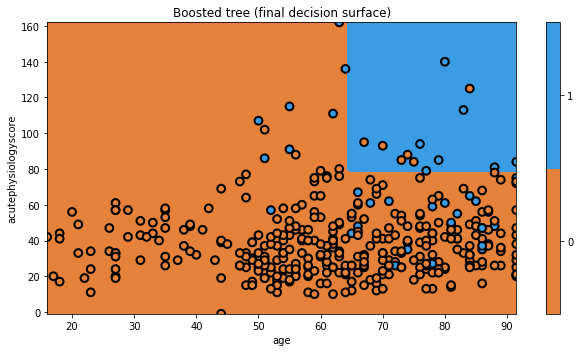
And that’s AdaBoost! There are a few tricks we have glossed over here, but you understand the general principle. We modified the data to focus on hard to classify observations. We can imagine this as a form of data resampling for each new tree.
For example, say we have three observations: A, B, and C, [A, B, C]. If we correctly classify observations [A, B], but incorrectly classify C, then AdaBoost involves building a new tree that focuses on C.
Equivalently, we could say AdaBoost builds a new tree using the dataset [A, B, C, C, C], where we have intentionally repeated observation C 3 times so that the algorithm thinks it is 3 times as important as the other observations. Makes sense?
Now we’ll move on to a different approach that also involves manipulating data to build new trees.
Key Points
An algorithm that performs somewhat poorly at a task - such as simple decision tree - is sometimes referred to as a “weak learner”.
With boosting, we create a combination of many weak learners to form a single “strong” learner.
Bagging
Overview
Teaching: 20 min
Exercises: 10 minQuestions
“Bagging is the shortened name for what?”
How can bagging improve model performance?
Objectives
Train a set of models using bagging.
Visualise the decision boundaries.
Bootstrap aggregation (“Bagging”)
Bootstrap aggregation, or “Bagging”, is another form of ensemble learning.
With boosting, we iteratively changed the dataset to have new trees focus on the “difficult” observations. Bagging involves the same approach, except we don’t selectively choose which observations to focus on, but rather we randomly select subsets of data each time.
Boosting aimed to iteratively improve our overall model with new trees. With bagging, we now build trees on what we hope are independent datasets.
Let’s take a step back, and think about a practical example. Say we wanted a good model of heart disease. If we saw researchers build a model from a dataset of patients from their hospital, we might think this would be sufficient. If the researchers were able to acquire a new dataset from new patients, and built a new model, we’d be inclined to feel that the combination of the two models would be better than any one individually.
This is the scenario that bagging aims to replicate, except instead of actually going out and collecting new datasets, we instead use “bootstrapping” to create new sets of data from our current dataset. If you are unfamiliar with bootstrapping, you can treat it as magic for now (and if you are familiar with the bootstrap, you already know that it is magic).
Let’s take a look at a simple bootstrap model.
np.random.seed(321)
clf = tree.DecisionTreeClassifier(max_depth=5)
mdl = ensemble.BaggingClassifier(base_estimator=clf, n_estimators=6)
mdl = mdl.fit(x_train.values, y_train.values)
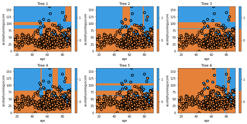
fig = plt.figure(figsize=[12,6])
for i, estimator in enumerate(mdl.estimators_):
ax = fig.add_subplot(2,3,i+1)
txt = 'Tree {}'.format(i+1)
glowyr.plot_model_pred_2d(estimator, x_train, y_train, title=txt)
We can see that each individual tree varies considerably. This is a result of using a random set of data to train the classifier.
# plot the final prediction
plt.figure(figsize=[8,5])
txt = 'Bagged tree (final decision surface)'
glowyr.plot_model_pred_2d(mdl, x_train, y_train, title=txt)
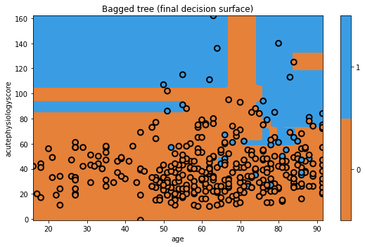
Not bad! Of course, since this is a simple dataset, we are not seeing that many dramatic changes between different models. Don’t worry, we’ll quantitatively evaluate them later.
Next up, a minor addition creates one of the most popular models in machine learning.
Key Points
“Bagging” is short name for bootstrap aggregation.
Bootstrapping is a data resampling technique.
Bagging is another method for combining multiple weak learners to create a strong learner.
Random forest
Overview
Teaching: 20 min
Exercises: 10 minQuestions
How can subselection of variables improve performance?
Objectives
Train a random forest model.
Visualise the decision boundaries.
Random Forest
In the previous example, we used bagging to randomly resample our data to generate “new” datasets. The Random Forest takes this one step further: instead of just resampling our data, we also select only a fraction of the features to include.
It turns out that this subselection tends to improve the performance of our models. The odds of an individual being very good or very bad is higher (i.e. the variance of the trees is increased), and this ends up giving us a final model with better overall performance (lower bias).
Let’s train the model.
np.random.seed(321)
mdl = ensemble.RandomForestClassifier(max_depth=5, n_estimators=6, max_features=1)
mdl = mdl.fit(x_train.values, y_train.values)

fig = plt.figure(figsize=[12,6])
for i, estimator in enumerate(mdl.estimators_):
    ax = fig.add_subplot(2,3,i+1)
    txt = 'Tree {}'.format(i+1)
    glowyr.plot_model_pred_2d(estimator, x_train, y_train, title=txt)
Question
a) When specifying the model, we set
max_featuresto1. All of the trees make decisions using both features, so it appears that our model is not respecting the argument. What is the explanation for this inconsistency?
b) What would you expect to see with amax_featuresof1AND amax_depthof1?
c) Repeat the plots with the new argument to check your answer to b. What do you see with respect to Age? Why?Answer
a) If it was true that setting
max_features=1as an argument led to trees with a single variable, we would not see the trees in our figure (which all make decisions based on both features). The explanation is that features are being limited at each split, not at the model level.
b) Settingmax_featuresto1limits our trees to a single split. We now see two sets of trees, some restricted to Acute Physiology Score and some restricted to Age.
c) Our trees decided against splitting on Age. The model was unable to find a single Age that led to improvement (based on its optimisation criteria).
Let’s look at final model’s decision surface.
plt.figure(figsize=[9,5])
txt = 'Random forest (final decision surface)'
glowyr.plot_model_pred_2d(mdl, x_train, y_train, title=txt)
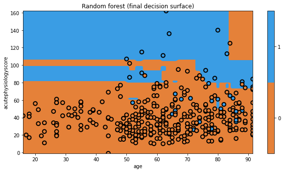
Again, the visualization doesn’t really show us the power of Random Forests, but we’ll quantitatively evaluate them soon enough.
Key Points
With Random Forest models, we resample data and use subsets of features.
Random Forest are powerful predictive models.
Gradient boosting
Overview
Teaching: 20 min
Exercises: 10 minQuestions
What is the state of the art in tree models?
Objectives
Train gradient boosted models.
Visualise the decision boundaries.
Gradient boosting
Last, but not least, we move on to gradient boosting. Gradient boosting, our last topic, elegantly combines concepts from the previous methods. As a “boosting” method, gradient boosting involves iteratively building trees, aiming to improve upon misclassifications of the previous tree. Gradient boosting also borrows the concept of sub-sampling the variables (just like Random Forests), which can help to prevent overfitting.
While it is too much to express in this tutorial, the biggest innovation in gradient boosting is that it provides a unifying mathematical framework for boosting models. The approach explicitly casts the problem of building a tree as an optimization problem, defining mathematical functions for how well a tree is performing (which we had before) and how complex a tree is. In this light, one can actually treat AdaBoost as a “special case” of gradient boosting, where the loss function is chosen to be the exponential loss.
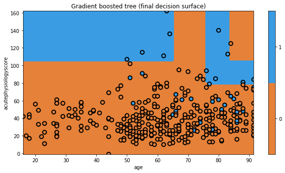
Let’s build a gradient boosting model.
np.random.seed(321)
mdl = ensemble.GradientBoostingClassifier(n_estimators=10)
mdl = mdl.fit(x_train.values, y_train.values)

plt.figure(figsize=[9,5])
txt = 'Gradient boosted tree (final decision surface)'
glowyr.plot_model_pred_2d(mdl, x_train, y_train, title=txt)
Key Points
As a “boosting” method, gradient boosting involves iteratively building trees, aiming to improve upon misclassifications of the previous tree.
Gradient boosting also borrows the concept of sub-sampling the variables (just like Random Forests), which can help to prevent overfitting.
The performance gains come at the cost of interpretability.
Performance
Overview
Teaching: 20 min
Exercises: 10 minQuestions
How well do our predictive models perform?
Objectives
Evaluate the performance of our different models.
Comparing model performance
We’ve now learned the basics of the various tree methods and have visualized most of them. Let’s finish by comparing the performance of our models on our held-out test data. Our goal, remember, is to predict whether or not a patient will survive their hospital stay using the patient’s age and acute physiology score computed on the first day of their ICU stay.
from sklearn import metrics

clf = dict()
clf['Decision Tree'] = tree.DecisionTreeClassifier(criterion='entropy', splitter='best').fit(x_train.values, y_train.values)
clf['Gradient Boosting'] = ensemble.GradientBoostingClassifier(n_estimators=10).fit(x_train.values, y_train.values)
clf['Random Forest'] = ensemble.RandomForestClassifier(n_estimators=10).fit(x_train.values, y_train.values)
clf['Bagging'] =  ensemble.BaggingClassifier(n_estimators=10).fit(x_train.values, y_train.values)
clf['AdaBoost'] =  ensemble.AdaBoostClassifier(n_estimators=10).fit(x_train.values, y_train.values)

fig = plt.figure(figsize=[10,10])

print('AUROC\tModel')
for i, curr_mdl in enumerate(clf):
    yhat = clf[curr_mdl].predict_proba(x_test.values)[:,1]
    score = metrics.roc_auc_score(y_test, yhat)
    print('{:0.3f}\t{}'.format(score, curr_mdl))
    ax = fig.add_subplot(3,2,i+1)
    glowyr. plot_model_pred_2d(clf[curr_mdl], x_test, y_test, title=curr_mdl)
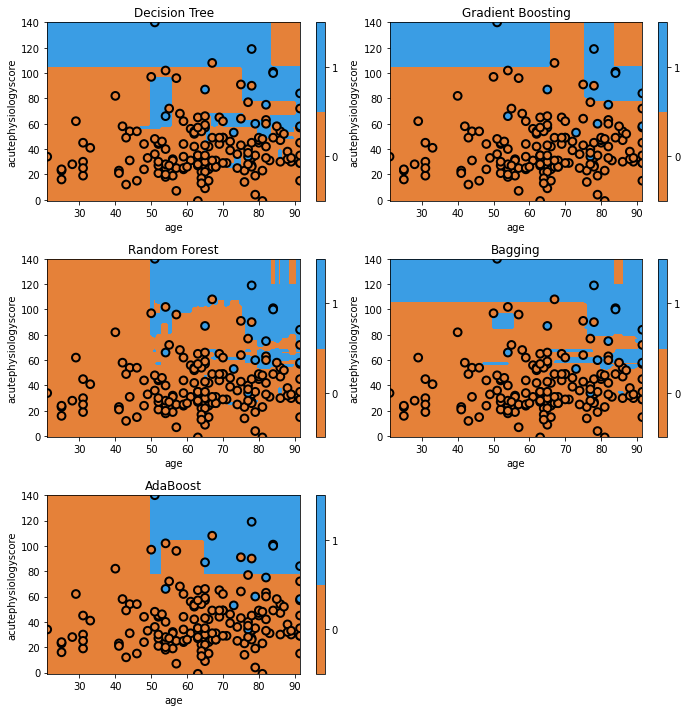
Here we can see that quantitatively, gradient boosting has produced the highest discrimination among all the models (~0.91). You’ll see that some of the models appear to have simpler decision surfaces, which tends to result in improved generalization on a held-out test set (though not always!).
To make appropriate comparisons, we should calculate 95% confidence intervals on these performance estimates. This can be done a number of ways. A simple but effective approach is to use bootstrapping, a resampling technique. In bootstrapping, we generate multiple datasets from the test set (allowing the same data point to be sampled multiple times). Using these datasets, we can then estimate the confidence intervals.
Key Points
There is a large performance gap between different types of tree.
Boosted models typically perform strongly.