All in One View
Content from Introduction
Last updated on 2026-06-02 | Edit this page
Overview
Questions
- “What is a Graphics Processing Unit?”
- “Can a GPU be used for anything other than graphics?”
- “For which kinds of tasks are GPUs faster than CPUs?”
Objectives
- “Explain the key architectural differences between CPU and GPU”
- “Estimate the performance speedup of running a computation on the GPU”
- “Use the terms host and device to distinguish CPU and GPU in the context of GPU programming”
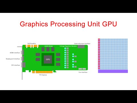
Graphics Processing Unit
The Graphics Processing Unit (GPU) is one of the components of a computer’s video card, together with specialized memory and different Input/Output (I/O) units. In the context of the video card, the GPU fulfills a role similar to the one that the Central Processing Unit (CPU) has in a general purpose computing system: it processes input data to generate some kind of output. In the traditional context of video cards, GPUs process data in order to render images on an output device, such as a screen. However, modern GPUs are general purpose computing devices that can be used to perform any kind of computation, and this is what we are going to do in this lesson.
Parallel by Design
But what is the reason to use GPUs to perform general purpose computation, when computers already have fast CPUs that are able to perform any kind of computation? One way to answer this question is to go back to the roots of what a GPU is designed to do: render images.
An image can be seen as a matrix of points called pixels (a portmanteau of the words picture and element), with each pixel representing the color the image should have in that particular point, and the traditional task performed by video cards is to produce the images a user will see on the screen. A single 4K UHD image contains more than 8 million pixels. For a GPU to render a continuous stream of 25 4K frames (images) per second, enough so that users do not experience delay in a videogame, movie, or any other video output, it must process over 200 million pixels per second. So GPUs are designed to render multiple pixels at the same time, and they are designed to do it efficiently. This design principle results in the GPU being, from a hardware point of view, very different from a CPU.
The CPU is a very general purpose device, good at different tasks, be they parallel or sequential in nature; it is also designed for interaction with the user, so it has to be responsive and guarantee minimal latency. In practice, we want our CPU to be available whenever we send it a new task. The result is a device where most of the silicon is used for memory caches and control-flow logic, not just compute units.
By contrast, most of the silicon on a GPU is actually used for compute units. The GPU does not need an overly complicated cache hierarchy, nor does it need complex control logic, because the overall goal is not to minimize the latency of any given thread, but to maximize the throughput of the whole computation. With many compute units available, the GPU can run massively parallel programs, programs in which thousands of threads are executed at the same time, while thousands more are ready for execution to hide the cost of memory operations.
A high-level introduction on the differences between CPU and GPU can also be found in the following YouTube video.
Speed Benefits
So, GPUs are massively parallel devices that can execute thousands of threads at the same time. But what does it mean in practice for the user? Why would anyone need to use a GPU to compute something that can be easily computed on a CPU? We can try to answer this question with an example.
Suppose we want to sort a large array in Python. Using NumPy, we first need to create an array of random single precision floating point numbers.
We then time the execution of the NumPy sort() function,
to see how long sorting this array takes on the CPU.
While the timing of this operation will differ depending on the system on which you run the code, these are the results for one experiment running on a Jupyter notebook on Google Colab.
OUTPUT
1.83 s ± 0 ns per loop (mean ± std. dev. of 1 run, 1 loop each)We now perform the same sorting operation, but this time we will be
using CuPy to execute the sort() function on the GPU. CuPy
is an open-source library for GPU computing in Python that mirrors the
NumPy API, meaning that most NumPy code can be run on the GPU simply by
replacing import numpy as np with
import cupy as cp. Under the hood, CuPy uses CUDA, NVIDIA’s
parallel computing platform, but users do not need to write any CUDA
code themselves to take advantage of it.
PYTHON
from cupyx.profiler import benchmark
import cupy as cp
data_gpu = cp.asarray(data)
execution_gpu = benchmark(cp.sort, (data_gpu,), n_repeat=10)
gpu_avg_time = np.average(execution_gpu.gpu_times)
print(f"{gpu_avg_time:.6f} s")
We also report the output, obtained on the same notebook on Google Colab; as always note that your result will vary based on the environment and GPU you are using.
OUTPUT
0.008949 sNotice that the first thing we need to do, is to copy the input data to the GPU. The distinction between data on the GPU and that on the host is a very important one that we will get back to later.
Host vs. Device
From now on we may also call the GPU the device, while we refer to other computations as taking place on the host. We’ll also talk about host memory and device memory, but much more on memory in later episodes!
Sorting an array using CuPy, and therefore using the GPU, is clearly much faster than using NumPy, but can we quantify how much faster? Having recorded the average execution time of both operations, we can then compute the speedup of using CuPy over NumPy. The speedup is defined as the ratio between the sequential (NumPy in our case) and parallel (CuPy in our case) execution times.
PYTHON
# using the experiment values from above: 1.83 s (NumPy) and 0.008949 s (CuPy)
speedup = 1.83 / 0.008949
print(speedup)
With the result of the previous operation being the following.
OUTPUT
204.49212202480723We can therefore say that just by using the GPU with CuPy to sort an
array of size 4096 * 4096 we achieved a performance
improvement of 204 times.
- “GPUs achieve high throughput by running thousands of threads in parallel, unlike CPUs which prioritise low latency”
- “In the context of GPU programming, we often refer to the GPU as the device and the CPU as the host”
- “Using GPUs to accelerate computation can provide large performance gains”
Content from Using your GPU with CuPy
Last updated on 2026-06-02 | Edit this page
Overview
Questions
- “How can I run NumPy code on the GPU?”
- “How can I copy NumPy arrays to the GPU?”
- “How do I reliably measure the execution time of GPU code?”
Objectives
- “Identify whether an array is stored in host or device memory”
- “Copy arrays between host and device memory using CuPy”
- “Select the appropriate CuPy or cupyx function to replace a NumPy or SciPy call”
- “Estimate the performance speedup of running a computation on the GPU”
- “Use
benchmark()fromcupyx.profilerto accurately time GPU code” - “Validate GPU results by comparing them against CPU results”
Introduction to CuPy
CuPy is a GPU array library that implements a subset of the NumPy and SciPy interfaces. Thanks to CuPy, people conversant with NumPy can very conveniently harvest the compute power of GPUs without writing code in GPU programming languages such as CUDA, OpenCL, and HIP.
From now on we can also use the word host to refer to the CPU on the laptop, desktop, or cluster node you are using as usual, and device to refer to the graphics card and its GPU.
Convolutions in Python
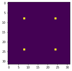
We start by generating an image using Python and NumPy code. We want to compute a convolution on this input image once on the host and once on the device, and then compare both the execution times and the results.
We can write and execute the following code on the host in an iPython
shell or a Jupyter notebook. The pixel values will be zero everywhere
except for a regular grid of single pixels having value one, very much
like a Dirac delta function; hence the input image is named
diracs.
PYTHON
import numpy as np
# Construct an image with repeated delta functions
diracs = np.zeros((2048, 2048))
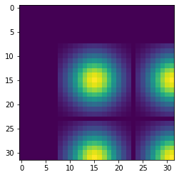
diracs[8::16,8::16] = 1We can display the top-left corner of the input image to get a feel for what it looks like, as follows:
PYTHON
import matplotlib.pyplot as plt
# Jupyter 'magic' command to render a Matplotlib image in the notebook
%matplotlib inline

# Display the image
# You can zoom in/out using the menu in the window that will appear
plt.imshow(diracs[0:32, 0:32])
plt.show()
and you should obtain the following image:
Gaussian convolutions
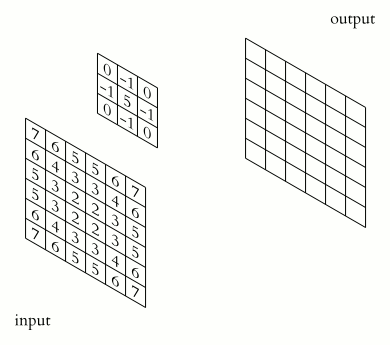
The illustration below shows an example of convolution (courtesy of Michael Plotke, CC BY-SA 3.0, via Wikimedia Commons). Looking at the terminology in the illustration, be forewarned that, inconveniently, the meaning of the word kernel is different when talking of mathematical convolutions and of codes for programming a GPU device. To know more about convolutions, we encourage you to check out this GitHub repository by Vincent Dumoulin and Francesco Visin, who show great animations.
In this course section, we will convolve our image with a 2D Gaussian function, having the general form:
\[G(x,y) = \frac{1}{2\pi \sigma^2} \exp\left(-\frac{x^2 + y^2}{2 \sigma^2}\right)\]
where \(x\) and \(y\) are distances from the origin, and \(\sigma\) controls the width of the curve. Since we can think of an image as a matrix of color values, the convolution of that image with a kernel generates a new matrix with different color values. In particular, convolving images with a 2D Gaussian kernel changes the value of each pixel into a weighted average of the neighboring pixels, thereby smoothing out the features in the input image.
Convolutions are frequently used in computer vision to filter images. For example, Gaussian convolution can be required before applying algorithms for edge detection, which are sensitive to the noise in the original image. To avoid conflicting vocabularies, in the remainder we refer to convolution kernels as filters.
Identifying the dataflow inherent in an algorithm is often useful. Say, if we want to square the numbers in a list, the operations on each item of the list are independent one of another. The dataflow of a one-to-one operation is called a map.

A convolution is slightly more complex because of a many-to-one dataflow, also known as a stencil.

GPUs are exceptionally well suited to compute algorithms that follow either dataflow.
Convolution on the CPU Using SciPy
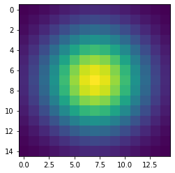
Let’s first construct and then display the Gaussian filter. Remember that we are still coding everything in standard Python, without using the GPU.
PYTHON
x, y = np.meshgrid(np.linspace(-2, 2, 15), np.linspace(-2, 2, 15))
dist = np.sqrt(x*x + y*y)
sigma = 1
origin = 0.000
gauss = np.exp(-(dist - origin)**2 / (2.0 * sigma**2))
plt.imshow(gauss)
plt.show()
The code above produces this image of a symmetrical two-dimensional Gaussian surface:
Now we are ready to compute the convolution on the host. Very conveniently, SciPy provides a method for convolutions. Let’s also record the time to perform this convolution and inspect the top-left corner of the convolved image, as follows:
PYTHON
from scipy.signal import convolve2d as convolve2d_cpu

convolved_image_cpu = convolve2d_cpu(diracs, gauss)
plt.imshow(convolved_image_cpu[0:32, 0:32])
plt.show()
%timeit -n 1 -r 1 convolve2d_cpu(diracs, gauss)
Obviously, the compute power of your CPU influences the actual execution time very much. We expect that to be in the region of a couple of seconds, as shown in the timing report below:
OUTPUT
2.4 s ± 0 ns per loop (mean ± std. dev. of 1 run, 1 loop each)Displaying just a corner of the image shows that the Gaussian filter has so much blurred the original pattern of ones surrounded by zeros that we end up with a regular pattern of Gaussians.
Convolution on the GPU Using CuPy
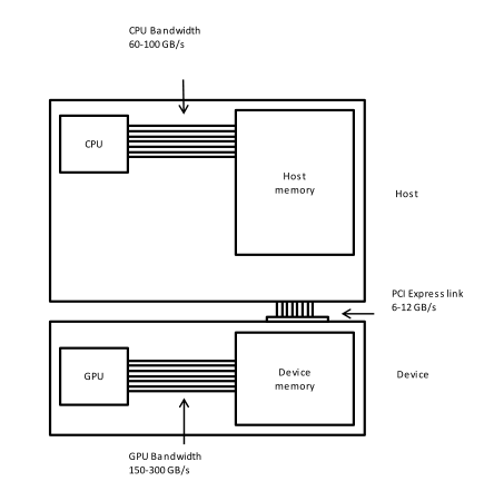
This is a lesson on GPU programming, so let’s use the GPU. In spite of being physically connected – typically with special interconnects – the CPU and the GPU do not share the same memory space. This picture depicts the different components of CPU and GPU and how they are connected:
This means that the array created with NumPy is physically stored in
the host’s memory and, therefore, is only available to the CPU. Since
our input image and convolution filter are not present in the device
memory yet, we need to copy them to the GPU before executing any code on
it. In practice, we use CuPy to copy the arrays diracs and
gauss from the host’s Random Access Memory (RAM) to the GPU
memory as follows:
Now it is time to compute the convolution on our GPU. Inconveniently,
SciPy does not offer methods running on GPUs. Hence, we import the
convolution function from a CuPy package aliased as cupyx.
Its sub-package cupyx.scipy
performs a selection of the SciPy operations. We will soon verify that
the convolution function of cupyx works out the same
calculations on the GPU as the convolution function of SciPy on the CPU.
In general, CuPy proper and NumPy are so similar one to another as are
the cupyx methods and SciPy; this is intended to invite
programmers already familiar with NumPy and SciPy to use the GPU for
computing. For now, let’s again record the execution time on the device
for the same convolution as the host, and compare the respective
performances.
PYTHON
from cupyx.scipy.signal import convolve2d as convolve2d_gpu

convolved_image_gpu = convolve2d_gpu(diracs_gpu, gauss_gpu)
%timeit -n 7 -r 1 convolved_image_gpu = convolve2d_gpu(diracs_gpu, gauss_gpu)
The execution time of the GPU convolution will depend very much on the hardware used, just as seen for the host. The timing using a NVIDIA Tesla T4 at Google Colab was:
OUTPUT
98.2 µs ± 0 ns per loop (mean ± std. dev. of 1 run, 7 loops each)This is way faster than the host: more than a 24000-fold performance improvement, or speedup. Impressive, but is that true?
Measuring performance
So far we used timeit to measure the performance of our
Python code, regardless of whether it was running on the CPU or was
GPU-accelerated. However, the execution on the GPU is
asynchronous: the Python interpreter immediately takes back
control of the program execution, while the GPU is still executing the
task. Therefore, the timing of timeit is not reliable.
Conveniently, cupyx provides the function
benchmark() that measures the actual execution time in the
GPU. The following code executes convolve2d_gpu() with the
appropriate arguments ten times, and stores inside the
.gpu_times attribute of the variable
benchmark_gpu the execution time of each run in
seconds.
PYTHON
from cupyx.profiler import benchmark

benchmark_gpu = benchmark(convolve2d_gpu, (diracs_gpu, gauss_gpu), n_repeat=10)
These measurements are also more stable and representative, because
benchmark() disregards the compile time and because the
repetitions warm up the GPU. We can then average the execution times, as
follows:
whereby the performance revisited is:
OUTPUT
0.020642 sWe now have a more reasonable, but still impressive, 116-fold speedup with respect to the execution on the host.
Challenge: convolution on the GPU without CuPy
Try to convolve the NumPy array diracs with the NumPy
array gauss directly on the GPU, that is, without CuPy
arrays. If this works, it will save us the time and effort of
transferring the arrays diracs and gauss to
the GPU.
We can call the GPU convolution function
convolve2d_gpu() directly with diracs and
gauss as argument:
However, this throws a long error message ending with:
OUTPUT
TypeError: Unsupported type <class 'numpy.ndarray'>Unfortunately, it is impossible to access directly from the GPU the NumPy arrays that live in the host RAM.
Validation
To check that the host and the device actually produced the same
output, we compare the two output arrays
convolved_image_gpu and convolved_image_cpu as
follows:
As you may have expected, the outcome of the comparison confirms that the results on the host and on the device are the same:
OUTPUT
array(True)Challenge: fairer comparison of CPU vs. GPU
Compute again the speedup achieved using the GPU, taking into account also the time spent transferring the data from the CPU to the GPU and back.
Hint: use the cp.asnumpy() method to copy a CuPy array
back to the host.
An effective strategy is to time the execution of a single Python function that groups the transfers to and from the GPU and the convolution, as follows:
PYTHON
def push_compute_pull():
diracs_gpu = cp.asarray(diracs)
gauss_gpu = cp.asarray(gauss)
convolved_image_gpu = convolve2d_gpu(diracs_gpu, gauss_gpu)
convolved_image_gpu_in_host = cp.asnumpy(convolved_image_gpu)
benchmark_gpu = benchmark(push_compute_pull, (), n_repeat=10)
gpu_execution_avg = np.average(benchmark_gpu.gpu_times)
print(f"{gpu_execution_avg:.6f} s")OUTPUT
0.035400 sThe speedup taking into account the data transfer decreased from 116
to 67. Nonetheless, accounting for the necessary data transfers is a
better and fairer way to compute performance speedups. As an aside, here
timeit would still provide correct measurements, because
the data transfers force the device and host to sync one with
another.
A shortcut: performing NumPy routines on the GPU
We saw in a previous challenge that we cannot launch the routines of
cupyx directly on NumPy arrays. In fact, we first needed to
transfer the data from the host to the device memory. Conversely, we
also encounter an error when we launch a regular SciPy routine, designed
to run on CPUs, on a CuPy array. Try out the following:
which results in
OUTPUT
...
...
...
TypeError: Implicit conversion to a NumPy array is not allowed.
Please use `.get()` to construct a NumPy array explicitly.
So, SciPy routines do not accept CuPy arrays as input. However,
instead of performing a 2D convolution, we can execute a simpler 1D
(linear) convolution that uses the NumPy routine
np.convolve() instead of a SciPy routine. To generate the
input appropriate to a linear convolution, we flatten our input image
from 2D to 1D using the method .ravel(). To generate a 1D
filter, we take the diagonal elements of our 2D Gaussian filter. Let’s
launch a linear convolution on the CPU with the following three
instructions:
PYTHON
diracs_1d_cpu = diracs.ravel()
gauss_1d_cpu = gauss.diagonal()
%timeit -n 1 -r 1 np.convolve(diracs_1d_cpu, gauss_1d_cpu)
A realistic execution time is:
OUTPUT
270 ms ± 0 ns per loop (mean ± std. dev. of 1 run, 1 loop each)After having performed this regular linear convolution on the host with NumPy, let’s try something bold. We transfer the 1D arrays to the device and do the convolution with the same NumPy routine, as follows:
PYTHON
diracs_1d_gpu = cp.asarray(diracs_1d_cpu)
gauss_1d_gpu = cp.asarray(gauss_1d_cpu)

benchmark_gpu = benchmark(np.convolve, (diracs_1d_gpu, gauss_1d_gpu), n_repeat=10)
gpu_execution_avg = np.average(benchmark_gpu.gpu_times)
print(f"{gpu_execution_avg:.6f} s")
You may be surprised that these commands do not throw any error.
Contrary to SciPy, NumPy routines accept CuPy arrays as input, even
though the latter exist only in GPU memory. Indeed, can you recall that
we validated our codes using a NumPy and a CuPy array as input of
np.allclose()? That worked for the same reason. The
CuPy documentation explains why NumPy routines can handle CuPy
arrays.
The last linear convolution has actually been performed on the GPU, and faster than the CPU:
OUTPUT
0.014529 sWith this NumPy shortcut and without much coding effort, we obtained a good 18-fold speedup.
A scientific application: image processing for radio astronomy
In this section, we will perform four classical steps in image processing for radio astronomy: determination of the background characteristics, segmentation, connected component labeling, and source measurements.
Import the FITS file
We import a 2048²-pixel image of the electromagnetic radiation at 150 MHz around the Galactic Center, as observed by the Indian Giant Metrewave Radio Telescope (GMRT).
The image is stored in this lesson’s
repository as a FITS file. The
astropy Python package enables us to read in this file and,
for compatibility with Python, convert the byte ordering from
the big to little endian, as follows:
Inspect the image
Let’s have a look at this image. Left and right in the data will be
swapped with the method np.fliplr() just to adhere to the
astronomical convention of the right ascension
increasing leftwards.
PYTHON
from matplotlib.colors import LogNorm

maxim = data.max()

fig = plt.figure(figsize=(50, 12.5))
ax = fig.add_subplot(1, 1, 1)
im_plot = ax.imshow(np.fliplr(data), cmap=plt.cm.gray_r, norm=LogNorm(vmin = maxim/10, vmax=maxim/100))
plt.colorbar(im_plot, ax=ax)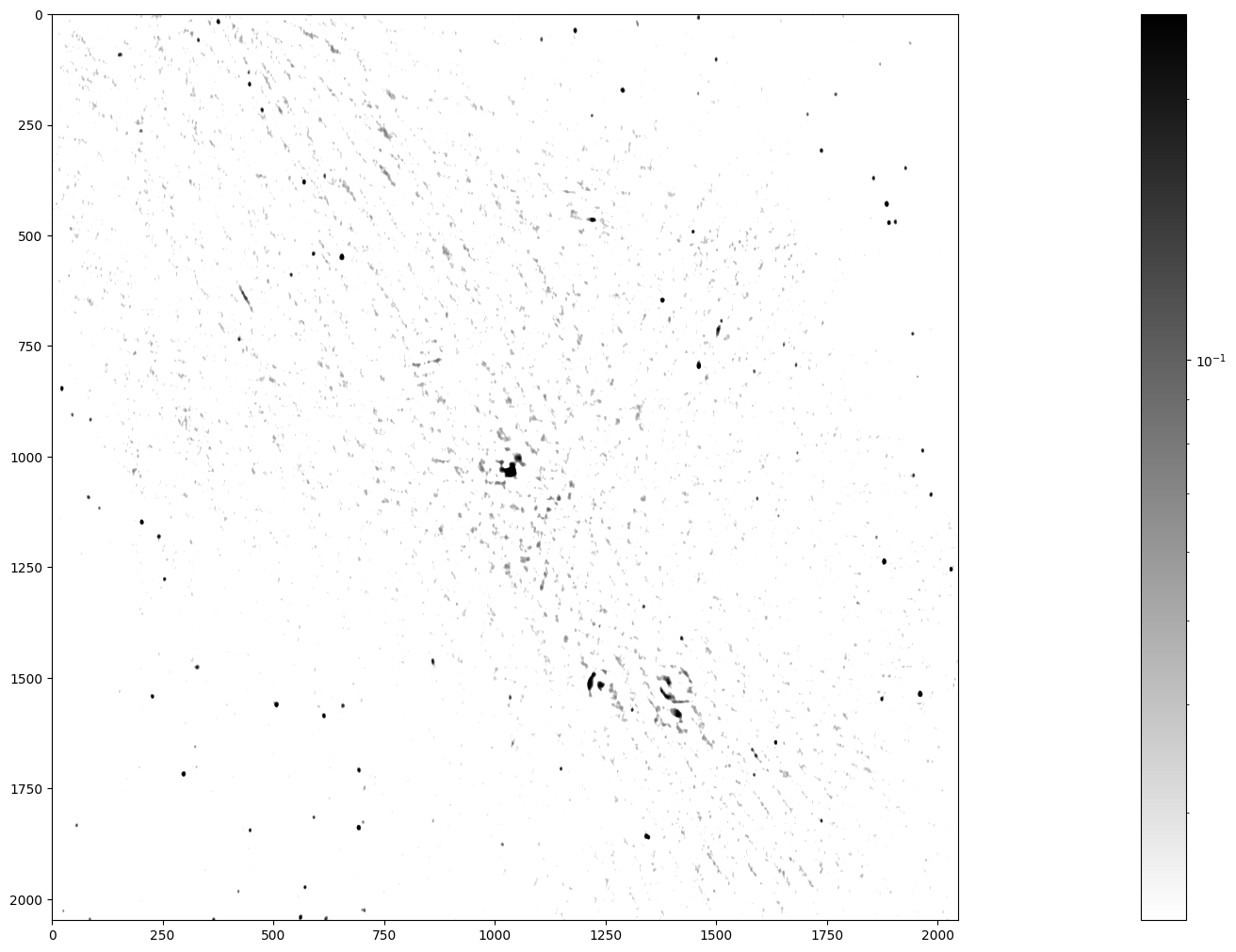
Stars, remnants of supernovas (massive exploded stars), and distant galaxies are possible radiation sources observed in this image. We can spot a few dozen radiation sources in fairly good quality in the lower left and upper right. In contrast, the quality is worse in the diagonal from the upper left to the lower right, because the radio telescope has a limited sensitivity and cannot look into large radiation sources. Nonetheless, you can notice the Galactic Center in the middle of the image and supernova shells as ring-like formations elsewhere.
The telescope accuracy has added background noise to the image. Yet, we want to identify all the radiation sources in this image, determine their positions, and measure their radiation fluxes. How can we then assert whether a high-intensity pixel is a peak of the noise or a genuine source? Assuming that the background noise is normally distributed with standard deviation \(\sigma\), the chance of its intensity being larger than 5\(\sigma\) is 2.9e-7. The chance of picking from our image of 2048² (4.2e6) pixels at least one that is so extremely bright because of noise is thus less than 50%.
Before moving on, let’s determine some summary statistics of the radiation intensity in the input image:
PYTHON
mean_ = data.mean()
median_ = np.median(data)
stddev_ = np.std(data)
max_ = np.amax(data)
print(f"mean = {mean_:.3e}, median = {median_:.3e}, stddev = {stddev_:.3e}, maximum = {max_:.3e}")
This gives (in Jy/beam):
OUTPUT
mean = 3.898e-04, median = 1.571e-05, stddev = 1.993e-02, maximum = 2.506e+00The maximum flux density is 2506 mJy/beam coming from the Galactic Center, the overall standard deviation 19.9 mJy/beam, and the median 1.57e-05 mJy/beam.
Step 1: Determining the characteristics of the background
First, we separate the background pixels from the source pixels using an iterative procedure called \(\kappa\)-\(\sigma\) clipping, which assumes that high intensity is more likely to result from genuine sources. We start from the standard deviation (\(\sigma\)) and the median (\(\mu_{1/2}\)) of all pixel intensities, as computed above. We then discard (clip) the pixels whose intensity is larger than \(\mu_{1/2} + 3\sigma\) or smaller than \(\mu_{1/2} - 3\sigma\). In the next pass, we compute again the median and standard deviation of the clipped set, and clip once more. We repeat these operations until no more pixels are clipped, that is, there are no outliers in the designated tails.
In the meantime, you may have noticed already that \(\kappa\)-\(\sigma\) clipping is a compute intensive task that could be implemented in a GPU. For the moment, let’s implement the algorithm with the NumPy code for a CPU, as follows:
PYTHON
# Flattening our 2D data makes subsequent steps easier
data_flat = data.ravel()

# Here is a kappa-sigma clipper for the CPU
def ks_clipper_cpu(data_flat):
    while True:
         med = np.median(data_flat)
         std = np.std(data_flat)
         clipped_below = data_flat.compress(data_flat > med - 3 * std)
         clipped_data = clipped_below.compress(clipped_below < med + 3 * std)
         if len(clipped_data) == len(data_flat):
             break
         data_flat = clipped_data
    return data_flat

data_clipped_cpu = ks_clipper_cpu(data_flat)
timing_ks_clipping_cpu = %timeit -o ks_clipper_cpu(data_flat)
fastest_ks_clipping_cpu = timing_ks_clipping_cpu.best
print(f"Fastest ks clipping time on CPU = {1000 * fastest_ks_clipping_cpu:.3e} ms.")
The performance is close to 1 s and, hopefully, can be sped up on the GPU.
OUTPUT
793 ms ± 17.2 ms per loop (mean ± std. dev. of 7 runs, 1 loop each)
Fastest ks clipping time on CPU = 7.777e+02 ms.
Finally, let’s see how the \(\kappa\)-\(\sigma\) clipping has influenced the summary statistics:
PYTHON
clipped_mean_ = data_clipped_cpu.mean()
clipped_median_ = np.median(data_clipped_cpu)
clipped_stddev_ = np.std(data_clipped_cpu)
clipped_max_ = np.amax(data_clipped_cpu)
print(f"mean of clipped = {clipped_mean_:.3e}, median of clipped = {clipped_median_:.3e}")
print(f"standard deviation of clipped = {clipped_stddev_:.3e}, maximum of clipped = {clipped_max_:.3e}")
The first-order statistics have become smaller, which reassures us
that data_clipped contains background pixels:
OUTPUT
mean of clipped = -1.945e-06, median of clipped = -9.796e-06
standard deviation of clipped = 1.334e-02, maximum of clipped = 4.000e-02
The standard deviation of the intensity in the background pixels will be the basis for the next step.
Challenge: \(\kappa\)-\(\sigma\) clipping on the GPU
Now that you know how the \(\kappa\)-\(\sigma\) clipping algorithm works, perform it on the GPU using CuPy. Compute the speedup, including the data transfer to and from the GPU.
PYTHON
def ks_clipper_gpu(data_flat):
    data_flat_gpu = cp.asarray(data_flat)
    data_gpu_clipped = ks_clipper_cpu(data_flat_gpu)
    return cp.asnumpy(data_gpu_clipped)

data_clipped_gpu = ks_clipper_gpu(data_flat)
timing_ks_clipping_gpu = benchmark(ks_clipper_gpu,
                                   (data_flat, ),
                                   n_repeat=10)
fastest_ks_clipping_gpu = np.amin(timing_ks_clipping_gpu.gpu_times)
print(f"{1000 * fastest_ks_clipping_gpu:.3e} ms")
OUTPUT
6.329e+01 msPYTHON
speedup_factor = fastest_ks_clipping_cpu/fastest_ks_clipping_gpu
print(f"The speedup factor for ks clipping is: {speedup_factor:.3e}")
OUTPUT
The speedup factor for ks clipping is: 1.232e+01Step 2: Segmenting the image
We have already estimated that clipping an image of 2048² pixels at the \(5 \sigma\) level yields a chance of less than 50% that at least one out of all the sources we detect is a noise peak. So let’s set the threshold at \(5\sigma\) and segment it.
First let’s check that the standard deviation from our clipper on the GPU is the same:
PYTHON
stddev_gpu_ = np.std(data_clipped_gpu)
print(f"standard deviation of background_noise = {stddev_gpu_:.4f} Jy/beam")
OUTPUT
standard deviation of background_noise = 0.0133 Jy/beamWe then apply the \(5 \sigma\) threshold to the image with this standard deviation:
PYTHON
threshold = 5 * stddev_gpu_
segmented_image = np.where(data > threshold, 1,  0)
timing_segmentation_CPU = %timeit -o np.where(data > threshold, 1,  0)
fastest_segmentation_CPU = timing_segmentation_CPU.best
print(f"Fastest CPU segmentation time = {1000 * fastest_segmentation_CPU:.3e} ms.")
OUTPUT
6.41 ms ± 55.3 µs per loop (mean ± std. dev. of 7 runs, 100 loops each)
Fastest CPU segmentation time = 6.294e+00 ms.
Step 3: Labeling the segmented data
This is called connected component labeling (CCL). It will replace pixel values in the segmented image - just consisting of zeros and ones - of the first connected group of pixels with the value 1 - so nothing changed, but just for that first group - the pixel values in the second group of connected pixels will all be 2, the third connected group of pixels will all have the value 3 etc.
This is a CPU code for connected component labeling.
PYTHON
from scipy.ndimage import label as label_cpu
labeled_image = np.empty(data.shape)
number_of_sources_in_image = label_cpu(segmented_image, output = labeled_image)
sigma_unicode = "\u03C3"
print(f"The number of sources in the image at the 5{sigma_unicode} level is {number_of_sources_in_image}.")

timing_CCL_CPU = %timeit -o label_cpu(segmented_image, output = labeled_image)
fastest_CCL_CPU = timing_CCL_CPU.best
print(f"Fastest CPU CCL time = {1000 * fastest_CCL_CPU:.3e} ms.")
This gives, on my machine:
OUTPUT
The number of sources in the image at the 5σ level is 185.
26.3 ms ± 965 µs per loop (mean ± std. dev. of 7 runs, 10 loops each)
Fastest CPU CCL time = 2.546e+01 ms.
Let’s not just accept the answer, and let’s do a sanity check. What are the values in the labeled image?
PYTHON
print(f"These are all the pixel values we can find in the labeled image: {np.unique(labeled_image)}")This should show the following output:
OUTPUT
These are all the pixel values we can find in the labeled image:
[  0.   1.   2.   3.   4.   5.   6.   7.   8.   9.  10.  11.  12.  13.
  14.  15.  16.  17.  18.  19.  20.  21.  22.  23.  24.  25.  26.  27.
  28.  29.  30.  31.  32.  33.  34.  35.  36.  37.  38.  39.  40.  41.
  42.  43.  44.  45.  46.  47.  48.  49.  50.  51.  52.  53.  54.  55.
  56.  57.  58.  59.  60.  61.  62.  63.  64.  65.  66.  67.  68.  69.
  70.  71.  72.  73.  74.  75.  76.  77.  78.  79.  80.  81.  82.  83.
  84.  85.  86.  87.  88.  89.  90.  91.  92.  93.  94.  95.  96.  97.
  98.  99. 100. 101. 102. 103. 104. 105. 106. 107. 108. 109. 110. 111.
 112. 113. 114. 115. 116. 117. 118. 119. 120. 121. 122. 123. 124. 125.
 126. 127. 128. 129. 130. 131. 132. 133. 134. 135. 136. 137. 138. 139.
 140. 141. 142. 143. 144. 145. 146. 147. 148. 149. 150. 151. 152. 153.
 154. 155. 156. 157. 158. 159. 160. 161. 162. 163. 164. 165. 166. 167.
 168. 169. 170. 171. 172. 173. 174. 175. 176. 177. 178. 179. 180. 181.
 182. 183. 184. 185.]
Step 4: Measuring the radiation sources
We are ready for the final step. We have been given observing time to make this beautiful image of the Galactic Center, we have determined its background statistics, we have separated actual cosmic sources from noise and now we want to measure these cosmic sources. What are their positions and what are their flux densities?
Again, the algorithms from scipy.ndimage help us to
determine these quantities. This is the CPU code for measuring our
sources.
PYTHON
from scipy.ndimage import center_of_mass as com_cpu
from scipy.ndimage import sum_labels as sl_cpu
all_positions = com_cpu(data, labeled_image,
                        range(1, number_of_sources_in_image+1))
all_integrated_fluxes = sl_cpu(data, labeled_image,
                               range(1, number_of_sources_in_image+1))

print (f'These are the ten highest integrated fluxes of the sources in my \n image: {np.sort(all_integrated_fluxes)[-10:]}')
which gives the Galactic Center as the most luminous source, which makes sense when we look at our image.
OUTPUT
These are the ten highest integrated fluxes of the sources in my image:
[ 38.90615184  41.91485894  43.02203498  47.30590784  51.23707351
  58.07289425  68.85673917  70.31223921  95.16443585 363.58937774]
Now we can try to measure the execution times for both algorithms, like this:
PYTHON
%%timeit -o
all_positions = com_cpu(data, labeled_image,
                        range(1, number_of_sources_in_image+1))
all_integrated_fluxes = sl_cpu(data, labeled_image,
                               range(1, number_of_sources_in_image+1))
which yields, on my machine:
OUTPUT
797 ms ± 9.32 ms per loop (mean ± std. dev. of 7 runs, 1 loop each)

<TimeitResult : 797 ms ± 9.32 ms per loop (mean ± std. dev. of 7 runs, 1 loop each)>
To collect the result from that timing in our next cell block, we
need a trick that uses the _ variable.
PYTHON
timing_source_measurements_CPU = _
fastest_source_measurements_CPU = timing_source_measurements_CPU.best
print(f"Fastest CPU set of source measurements = {1000 * fastest_source_measurements_CPU:.3e} ms.")
which yields
OUTPUT
Fastest CPU set of source measurements = 7.838e+02 ms.Challenge: putting it all together
Combine the first two steps of image processing for astronomy, i.e. determining background characteristics e.g. through \(\kappa\)-\(\sigma\) clipping and segmentation into a single function, that works for both CPU and GPU. Next, write a function for connected component labeling and source measurements on the GPU and calculate the overall speedup factor for the combined four steps of image processing in astronomy on the GPU relative to the CPU. Finally, verify your output by comparing with the previous output, using the CPU.
PYTHON
def first_two_steps_for_both_CPU_and_GPU(data):
    data_flat = data.ravel()
    data_clipped = ks_clipper_cpu(data_flat)
    stddev_ = np.std(data_clipped)
    threshold = 5 * stddev_
    segmented_image = np.where(data > threshold, 1,  0)
    return segmented_image

def ccl_and_source_measurements_on_CPU(data_CPU, segmented_image_CPU):
    labeled_image_CPU = np.empty(data_CPU.shape)
    number_of_sources_in_image = label_cpu(segmented_image_CPU,
                                           output= labeled_image_CPU)
    all_positions = com_cpu(data_CPU, labeled_image_CPU,
                            np.arange(1, number_of_sources_in_image+1))
    all_fluxes = sl_cpu(data_CPU, labeled_image_CPU,
                        np.arange(1, number_of_sources_in_image+1))
    return np.array(all_positions), np.array(all_fluxes)

CPU_output = ccl_and_source_measurements_on_CPU(data,
                                            first_two_steps_for_both_CPU_and_GPU(data))

timing_complete_processing_CPU =  benchmark(
                                            ccl_and_source_measurements_on_CPU,
                                            (data,
                                            first_two_steps_for_both_CPU_and_GPU(data)),                                             n_repeat=10)

fastest_complete_processing_CPU = np.amin(timing_complete_processing_CPU.cpu_times)

print(f"The four steps of image processing for astronomy take {1000 * fastest_complete_processing_CPU:.3e} ms\n on our CPU.")

from cupyx.scipy.ndimage import label as label_gpu
from cupyx.scipy.ndimage import center_of_mass as com_gpu
from cupyx.scipy.ndimage import sum_labels as sl_gpu

def ccl_and_source_measurements_on_GPU(data_GPU, segmented_image_GPU):
    labeled_image_GPU = cp.empty(data_GPU.shape)
    number_of_sources_in_image = label_gpu(segmented_image_GPU,
                                           output= labeled_image_GPU)
    all_positions = com_gpu(data_GPU, labeled_image_GPU,
                            cp.arange(1, number_of_sources_in_image+1))
    all_fluxes = sl_gpu(data_GPU, labeled_image_GPU,
                        cp.arange(1, number_of_sources_in_image+1))
    # This seems redundant, but we want to return ndarrays (Numpy)
    # and what we have are lists.
    # These first have to be converted to
    # Cupy arrays before they can be converted to Numpy arrays.
    return (cp.asnumpy(cp.asarray(all_positions)),
            cp.asnumpy(cp.asarray(all_fluxes)))

GPU_output = ccl_and_source_measurements_on_GPU(cp.asarray(data), first_two_steps_for_both_CPU_and_GPU(cp.asarray(data)))

timing_complete_processing_GPU =  benchmark(ccl_and_source_measurements_on_GPU, (cp.asarray(data), first_two_steps_for_both_CPU_and_GPU(cp.asarray(data))), n_repeat=10)

fastest_complete_processing_GPU = np.amin(timing_complete_processing_GPU.gpu_times)

print(f"The four steps of image processing for astronomy take {1000 * fastest_complete_processing_GPU:.3e} ms\n on our GPU.")

overall_speedup_factor = fastest_complete_processing_CPU /                         fastest_complete_processing_GPU
print(f"This means that the overall speedup factor GPU vs CPU equals: {overall_speedup_factor:.3e}\n")

all_positions_agree = np.allclose(CPU_output[0], GPU_output[0])
print(f"The CPU and GPU positions agree: {all_positions_agree}\n")

all_fluxes_agree = np.allclose(CPU_output[1], GPU_output[1])
print(f"The CPU and GPU fluxes agree: {all_fluxes_agree}\n")
OUTPUT
The four steps of image processing for astronomy take 1.060e+03 ms on our CPU.
The four steps of image processing for astronomy take 5.770e+01 ms on our GPU.
This means that the overall speedup factor GPU vs CPU equals: 1.838e+01

The CPU and GPU positions agree: True

The CPU and GPU fluxes agree: True- “CuPy provides GPU-accelerated versions of many NumPy and SciPy functions.”
- “Always have CPU and GPU versions of your code so that you can compare performance, as well as validate your code.”
- “GPU execution is asynchronous; use
cupyx.profiler.benchmark()rather thantimeitfor accurate measurements.”
Content from Using PyTorch for GPU Computing
Last updated on 2026-06-02 | Edit this page
Overview
Questions
- “How can we create and manipulate PyTorch tensors on a GPU?”
- “How can we move data between NumPy, CPU tensors, and GPU tensors?”
- “Why can PyTorch be useful for general-purpose GPU computing?”
Objectives
- “Create PyTorch tensors and apply operations.”
- “Understand the
@torch.compiledecorator and its limitations.” - “Compare the performance of PyTorch against other solutions.”
Introduction to PyTorch
PyTorch, often referred to as just torch, is a popular open-source Python library commonly used for machine learning and AI. It provides many features for working with N-dimensional arrays (called tensors), automatic differentiation, neural networks, and GPU acceleration. PyTorch was originally developed by Meta and is now maintained by the PyTorch Foundation, which is part of the Linux Foundation.
You can read more about PyTorch here: https://pytorch.org/
PyTorch has many features related to AI and training neural networks. However, in this episode, we will focus on running general-purpose code on the GPU using tensors.
Getting started
First, we need to import torch:
Next, we can check whether PyTorch detects a GPU:
After this, we can create a device and print its name. The device
determines where PyTorch stores data and performs computations. In our
case, we will use cuda:0, which refers to the NVIDIA GPU
with index 0.
PYTHON
# Initialize the device
device = torch.device("cuda:0")

# Print the device name
name = torch.cuda.get_device_name(device)
print("GPU detected:", name)
This shows the full name of the GPU. For example:
OUTPUT
GPU detected: NVIDIA A100-SXM4-40GB MIG 3g.20gbNext, we create a tensor. A tensor is similar to a NumPy array. We
can create a tensor using torch.tensor, and place it on the
GPU using device=device.
PYTHON
# Create a tensor on the GPU containing the numbers [1, 2, 3, 4]
x = torch.tensor([1.0, 2, 3, 4], device=device)

# Print the number of elements
print(x.numel())

# Print the data type of the elements
print(x.dtype)
This should print 4 and torch.float32.
Notice that PyTorch’s default floating-point type is usually 32-bit,
while NumPy often defaults to 64-bit floating-point numbers. This is
useful on GPUs, where 32-bit operations are usually faster. You can
change the default floating-point dtype using
torch.set_default_dtype(torch.float64), which can be useful
when matching NumPy code.
Working with tensors
To convert a NumPy array into a PyTorch tensor, we can use
torch.from_numpy. Note that the resulting PyTorch tensor
will not copy the data; instead, it shares the same memory with the
NumPy array. This means that modifying the PyTorch tensor will also
change the contents of the original NumPy array.
To convert a tensor back into a NumPy array, we can use
tensor.cpu().numpy(). Since NumPy arrays always live in CPU
memory, CUDA tensors must first be copied back to the CPU using
.cpu().
PYTHON
import numpy as np

# Create NumPy array
a = np.array([5, 6, 7, 8])

# Convert NumPy -> PyTorch tensor (CPU)
b = torch.from_numpy(a)

# Copy CPU -> GPU
c = b.to(device)

# Copy GPU -> CPU
d = c.cpu()

# Convert back to NumPy array
e = d.numpy()

# They should be equal
print(np.all(a == e))
This should print True, since the conversion from NumPy
to PyTorch and back is lossless.
There are also many ways to create a tensor directly on the GPU. Many are similar to functions in NumPy. These functions create the data directly in GPU memory, without copying it from the CPU. Here are some examples.
PYTHON
# Gives [0.0, 0.0, 0.0, 0.0, ...]
a = torch.zeros(10, device=device)

# Gives [1.0, 1.0, 1.0, 1.0, ...]
b = torch.ones(10, device=device)

# Gives [42.0, 42.0, 42.0, 42.0, ...]
c = torch.full((10,), 42.0, device=device)

# Gives [0.3226, 0.7758, 0.6456, ...]
d = torch.rand(10, device=device)

# Gives an uninitialized array
e = torch.empty(10, device=device)

# Gives [0, 1, 2, 3, 4, ...]
f = torch.arange(10, device=device)

# Gives [0.0000, 0.1111, 0.2222, 0.3333, ..., 1.0000]
g = torch.linspace(0, 1, 10, device=device)
Tensors can be multi-dimensional. They can be 1-dimensional (vectors), 2-dimensional (matrices), 3-dimensional (cubes), and so on.
PYTHON
# This is a vector of length 3
x = torch.rand(3, device=device)

# This is a matrix of size 3x3
y = torch.rand((3, 3), device=device)

# This is a cube of size 3x3x3
z = torch.rand((3, 3, 3), device=device)
Slicing is also supported, similar to NumPy. For example,
m[i, :] gives the \(i\)-th
row and m[:, j] gives the \(j\)-th column of a matrix m.
The result of slicing a tensor is again a tensor. Note that modifying
this slice will also modify the original tensor, as it is a view.
PYTHON
x = torch.rand(2, 3, device=device)

# Print the matrix
print("before:", x)

# Modify the first row
x[0, :] = 0

# Print the matrix
print("after:", x)
OUTPUT
before: tensor([[0.9707, 0.2220, 0.9106], [0.2907, 0.4936, 0.1780]], device='cuda:0')
after: tensor([[0.0000, 0.0000, 0.0000], [0.2907, 0.4936, 0.1780]], device='cuda:0')
Tensors also support many mathematical operations.
PYTHON
x = torch.ones(5, device=device)
y = torch.arange(5, device=device)

print("x+y:", x + y)
print("x-y:", x - y)
print("x*y:", x * y)
print("x/y:", x / y)
print("sqrt:", torch.sqrt(y))
print("exp:", torch.exp(y))
print("sin:", torch.sin(y))
OUTPUT
x+y: tensor([1., 2., 3., 4., 5.], device='cuda:0')
x-y: tensor([ 1.,  0., -1., -2., -3.], device='cuda:0')
x*y: tensor([0., 1., 2., 3., 4.], device='cuda:0')
x/y: tensor([   inf, 1.0000, 0.5000, 0.3333, 0.2500], device='cuda:0')
sqrt: tensor([0.0000, 1.0000, 1.4142, 1.7321, 2.0000], device='cuda:0')
exp: tensor([ 1.0000,  2.7183,  7.3891, 20.0855, 54.5982], device='cuda:0')
sin: tensor([ 0.0000,  0.8415,  0.9093,  0.1411, -0.7568], device='cuda:0')
Be aware that you cannot mix NumPy arrays and GPU tensors in these
operations. To do this, you either need to use .cpu() to
convert your GPU tensor into a CPU tensor or, alternatively, copy your
NumPy array into a GPU tensor.
PYTHON
x = torch.rand(5, device=device)
y = np.arange(5)

# This is not allowed
try:
    print(x + y)
except Exception as e:
    print("error:", e)

# This returns a tensor on the CPU
print("CPU:", x.cpu() + y)

# This returns a tensor on the GPU
print("GPU:", x + torch.tensor(y, device=device))
OUTPUT
error: can't convert cuda:0 device type tensor to numpy. Use Tensor.cpu() to copy the tensor to host memory first.
CPU: tensor([0.6511, 1.7587, 2.4972, 3.3509, 4.5963])
GPU: tensor([0.6511, 1.7587, 2.4972, 3.3509, 4.5963], device='cuda:0')
Example Using N-Body Simulation
Now, we will consider a larger example of how to use PyTorch. For
this example, we consider n random planetary bodies and
calculate the total gravitational force that each body experiences from
the other bodies using Newton’s
law of universal gravitation.
First, we generate n random planets in a 2D plane. The
x and y coordinates are chosen randomly in the
range \([0, 1]\).
PYTHON
n = 10
position = torch.rand((2, n), device=device)
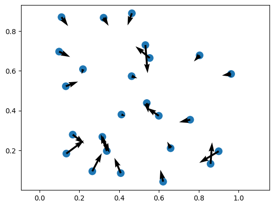
mass = torch.rand(n, device=device) + 100Let’s plot the positions of the planets.
PYTHON
%matplotlib inline
import matplotlib.pyplot as plt

plt.axis("equal")
plt.scatter(
    position[0,:].cpu(),
    position[1,:].cpu(),
    s=mass.cpu()
)
plt.show()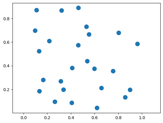
The force on planet \(i\) is given by the following equation:
\(\mathbf{F}_i = \sum_{j=1, j \neq i}^{N} G \frac{m_i m_j}{\|\mathbf{p}_j - \mathbf{p}_i\|^2} \left(\frac{\mathbf{p}_j - \mathbf{p}_i}{\|\mathbf{p}_j - \mathbf{p}_i\|}\right)\)
Now, we can define a function that computes these forces between the planets.
PYTHON
G = 6.67e-11

def calculate_forces(pos, mass):
    # diff[:, i, j] = pos_j - pos_i
    diff = pos[:, None, :] - pos[:, :, None] # (2, N, N)

    # dist[i, j] = ||pos_j - pos_i||
    dist = diff.norm(dim=0)        # (N, N)
    direction = diff / dist

    # Force on i from j: F_ij = G * m_i * m_j * r_ij / |r_ij|^2
    forces = G * mass[:, None] * mass[None, :] / dist**2
    return (direction * forces[None, :, :]).nansum(dim=2)  # (2, N)
Finally, we can plot the results.
PYTHON
forces = calculate_forces(position, mass)

plt.axis("equal")
plt.scatter(
    position[0,:].cpu(),
    position[1,:].cpu(),
    s=mass.cpu()
)

plt.quiver(
  position[0,:].cpu(),
  position[1,:].cpu(),
  forces[0,:].cpu(),
  forces[1,:].cpu()
)
Using torch.compile
An important feature introduced in PyTorch 2.0 is the @torch.compile
decorator. This decorator can be applied to a Python function and tells
PyTorch to compile the tensor operations inside the function into a more
optimized version before executing it. Instead of running the function
line by line in Python, PyTorch analyzes the operations inside the
function and builds a more efficient computation graph. It can then
apply various optimizations, such as fusing multiple operations
together, reducing memory usage, and generating more efficient GPU
kernels.
This process can significantly improve performance, especially for functions that perform many tensor operations. The compiled function can therefore run much faster than the original Python version while keeping the code easy to read and write.
Below is a simple example. We create two large tensors on the GPU and
define a function that performs several mathematical operations on them.
By adding the @torch.compile decorator, PyTorch will
attempt to optimize the function automatically.
PYTHON
@torch.compile
def compute(a, b):
    return (a + b) + torch.sin(a) * torch.cos(b)

a = torch.rand(1_000_000, device=device)
b = torch.rand(1_000_000, device=device)
c = compute(a, b)

print("result:", c)
This lets PyTorch optimize the compute function as a
whole and makes the code faster than running the operations separately.
It accomplishes this by tracing through your Python code and looking for
PyTorch operations.
For example, to see what PyTorch is doing internally, we can use
set_logs, which prints what happens under the hood.
This generates a large amount of output about the internals of PyTorch. You do not need to understand all the output. However, among this output is the following:
OUTPUT
...
[__graph_code] TRACED GRAPH
[__graph_code]  ===== __compiled_fn_139_120d693e_cd49_4b9d_8ed2_fa7094feea70 =====
[__graph_code]  /home/user/.local/lib/python3.13/site-packages/torch/fx/_lazy_graph_module.py class GraphModule(torch.nn.Module):
[__graph_code]     def forward(self, L_a_: "f64[1000000][1]cuda:0", L_b_: "f64[1000000][1]cuda:0"):
[__graph_code]         l_a_ = L_a_
[__graph_code]         l_b_ = L_b_
[__graph_code]         torch.sin(a) * torch.cos(b)
[__graph_code]         add: "f64[1000000][1]cuda:0" = l_a_ + l_b_
[__graph_code]         sin: "f64[1000000][1]cuda:0" = torch.sin(l_a_);  l_a_ = None
[__graph_code]         cos: "f64[1000000][1]cuda:0" = torch.cos(l_b_);  l_b_ = None
[__graph_code]         mul: "f64[1000000][1]cuda:0" = sin * cos;  sin = cos = None
[__graph_code]         add_1: "f64[1000000][1]cuda:0" = add + mul;  add = mul = None
[__graph_code]         return (add_1,)
...
This part shows how PyTorch has traced our function
compute as a graph of operations.
OUTPUT
...
[__kernel_code] @triton.jit
[__kernel_code] def triton_poi_fused_add_cos_mul_sin_0(in_ptr0, in_ptr1, out_ptr0, xnumel, XBLOCK : tl.constexpr):
[__kernel_code]     xnumel = 1000000
[__kernel_code]     xoffset = tl.program_id(0) * XBLOCK
[__kernel_code]     xindex = xoffset + tl.arange(0, XBLOCK)[:]
[__kernel_code]     xmask = xindex < xnumel
[__kernel_code]     x0 = xindex
[__kernel_code]     tmp0 = tl.load(in_ptr0 + (x0), xmask)
[__kernel_code]     tmp1 = tl.load(in_ptr1 + (x0), xmask)
[__kernel_code]     tmp2 = tmp0 + tmp1
[__kernel_code]     tmp3 = libdevice.sin(tmp0)
[__kernel_code]     tmp4 = libdevice.cos(tmp1)
[__kernel_code]     tmp5 = tmp3 * tmp4
[__kernel_code]     tmp6 = tmp2 + tmp5
[__kernel_code]     tl.store(out_ptr0 + (x0), tmp6, xmask)
...
This part shows that PyTorch automatically generated a GPU
kernel named triton_poi_fused_add_cos_mul_sin_0
that performs all operations in one go, instead of having separate
functions for each operation. The generated kernel uses Triton, a
Python-based language and compiler for GPU programming.
There are certain limitations to @torch.compile. For
example, the inputs and outputs can only be PyTorch tensors, and you
must be careful with loops (for statements) and
conditionals (if statements). For more information, see the
guide
on the torch.compile programming model.
As an example, consider the following function that scales a tensor
by 2 if the sum is positive and -2 otherwise.
Note that we pass the fullgraph=True option to force
PyTorch to raise an error if it cannot compile.
PYTHON
import torch

@torch.compile(fullgraph=True)
def fail_example(x):
    if x.sum() > 0:
        return x * 2
    else:
        return x * -2

fail_example(torch.rand(100, device=device))
This results in the following error:
OUTPUT
Unsupported: Data-dependent branching
  Explanation: Detected data-dependent branching (e.g. `if my_tensor.sum() > 0:`). Dynamo does not support tracing dynamic control flow.
  Hint: This graph break is fundamental - it is unlikely that Dynamo will ever be able to trace through your code. Consider finding a workaround.
  Hint: Use `torch.cond` to express dynamic control flow.

  Developer debug context: attempted to jump with TensorVariable()

 For more details about this graph break, please visit: https://meta-pytorch.github.io/compile-graph-break-site/gb/gb0170.html
The problem here is that PyTorch cannot statically determine whether
to execute x * 2 or x * -2, as this is
dependent on the runtime value of x.sum().
Instead, for this example, we can use torch.where to
select between them instead of having an if statement.
Comparison of performance
Let’s measure the time of our calculate_forces function
with and without @torch.compile to compare the
performance.
First, we import %gpu_timeit from
cupyx.
Next, we call our function with 10,000 planets.
PYTHON
n = 10_000
pos = torch.rand(2, n, device=device)
mass = torch.rand(n, device=device)

%gpu_timeit -n50 calculate_forces(pos, mass)
OUTPUT
run:    CPU:   177.674 us   +/-  9.926 (min:   171.843 / max:   241.492) us
      GPU-0: 21880.586 us   +/- 11.218 (min: 21849.089 / max: 21906.431) us
The execution time on the GPU is around 21.880 milliseconds.
We can use @torch.compile to speed things up! Note how
@torch.compile works recursively: if a function is
compiled, all called functions are also compiled.
PYTHON
n = 10_000
pos = torch.rand(2, n, device=device)
mass = torch.rand(n, device=device)

@torch.compile
def calculate_forces_fast(pos, mass):
    return calculate_forces(pos, mass)

forces = calculate_forces_fast(pos, mass);

%gpu_timeit -n50 calculate_forces_fast(pos, mass)
OUTPUT
run:    CPU:   114.750 us   +/- 23.757 (min:   106.006 / max:   277.980) us
      GPU-0:  4008.182 us   +/- 22.778 (min:  3997.696 / max:  4164.608) us
This time it takes around 4.008 milliseconds, a speedup of 5.5x over the original version!
As a comparison, we can also run the same function on the CPU using PyTorch:
PYTHON
n = 10_000
pos = torch.rand(2, n, device="cpu")
mass = torch.rand(n, device="cpu")

%gpu_timeit -n1 calculate_forces_fast(pos, mass)
OUTPUT
run: CPU: 608562.989 us GPU-0: 608638.977 usThe CPU takes 608.563 milliseconds, meaning our GPU is around 152x faster than our CPU for this particular calculation!
Challenge
Measure the performance of calculate_forces_fast for
different numbers of planets. For example, n = 2500,
n = 5000, n = 10_000, and
n = 20_000. What timings do you expect? What do you
get?
The following times were measured (on your system they might be different!).
OUTPUT
421.274 us
1354.342 us
4965.478 us
18965.095 us
The results show that each time we double n, the
execution time quadruples. This happens as the number of pairwise
interactions between \(n\) planets
equals \(n^2\).
- “PyTorch tensors can be created and manipulated directly on the GPU”
- “Use
.to(device)to move data between CPU and GPU, and.cpu().numpy()to convert back to NumPy” - “The
@torch.compiledecorator can significantly speed up tensor operations by fusing them into optimized GPU kernels”
Content from Accelerate your Python code with Numba
Last updated on 2026-06-02 | Edit this page
Overview
Questions
- “How can I run my own Python functions on the GPU?”
Objectives
- “Learn how to use Numba decorators to improve the performance of your Python code.”
- “Run your first application on the GPU.”
Using Numba to execute Python code on the GPU
Numba is a Python library that “translates Python functions to optimized machine code at runtime using the industry-standard LLVM compiler library”. You might want to try it to speed up your code on a CPU. However, Numba can also translate a subset of the Python language into CUDA, which is what we will be using here. So the idea is that we can do what we are used to, i.e. write Python code and still benefit from the speed that GPUs offer us.
We want to compute all prime numbers - i.e. numbers that have only 1 or themselves as exact divisors - between 1 and 10000 on the CPU and see if we can speed it up, by deploying a similar algorithm on a GPU. This is code that you can find on many websites. Small variations are possible, but it will look something like this:
PYTHON
def find_all_primes_cpu(upper):
    all_prime_numbers = []
    for num in range(0, upper):
        prime = True
        for i in range(2, (num // 2) + 1):
            if (num % i) == 0:
                prime = False
                break
        if prime:
            all_prime_numbers.append(num)
    return all_prime_numbers
Calling find_all_primes_cpu(10_000) will return all
prime numbers between 1 and 10000 as a list. Let us time it:
You will probably find that find_all_primes_cpu takes
several hundreds of milliseconds to complete:
OUTPUT
176 ms ± 0 ns per loop (mean ± std. dev. of 1 run, 10 loops each)As a quick sidestep, add Numba’s JIT (Just in Time compilation)
decorator to the find_all_primes_cpu function. You can
either add it to the function definition or to the call, so either in
this way:
PYTHON
from numba import jit

@jit(nopython=True)
def find_all_primes_cpu(upper):
    all_prime_numbers = []
    for num in range(0, upper):
        prime = True
        for i in range(2, (num // 2) + 1):
            if (num % i) == 0:
                prime = False
                break
        if prime:
            all_prime_numbers.append(num)
    return all_prime_numbers

%timeit -n 10 -r 1 find_all_primes_cpu(10_000)
or in this way:
PYTHON
from numba import jit

upper = 10_000
%timeit -n 10 -r 1 jit(nopython=True)(find_all_primes_cpu)(upper)
which can give you a timing result similar to this:
OUTPUT
69.5 ms ± 0 ns per loop (mean ± std. dev. of 1 run, 10 loops each)So twice as fast, by using a simple decorator. The speedup is much
larger for upper = 100_000, but that takes a little too
much waiting time for this course. Despite the
jit(nopython=True) decorator the computation is still
performed on the CPU. Let us move the computation to the GPU. There are
a number of ways to achieve this, one of them is the usage of the
jit(device=True) decorator, but it depends very much on the
nature of the computation. Let us write our first GPU kernel which
checks if a number is a prime, using the cuda.jit
decorator, so different from the jit decorator for CPU
computations. It is essentially the inner loop of
find_all_primes_cpu:
PYTHON
from numba import cuda

@cuda.jit
def check_prime_gpu_kernel(num, result):
   result[0] =  num
   for i in range(2, (num // 2) + 1):
       if (num % i) == 0:
           result[0] = 0
           break
A number of things are worth noting. CUDA kernels do not return anything, so you have to supply for an array to be modified. All arguments have to be arrays, if you work with scalars, make them arrays of length one. This is the case here, because we check if a single number is a prime or not. Let us see if this works:
PYTHON
import numpy as np

result = np.zeros((1), np.int32)
check_prime_gpu_kernel[1, 1](11, result)
print(result[0])
check_prime_gpu_kernel[1, 1](12, result)
print(result[0])
If we have not made any mistake, the first call should return “11”, because 11 is a prime number, while the second call should return “0” because 12 is not a prime:
OUTPUT
11
0
Note the extra arguments in square brackets - [1, 1] -
that are added to the call of check_prime_gpu_kernel: these
indicate the number of threads we want to run on the GPU. While this is
an important argument, we will explain it later and for now we can keep
using 1.
Challenge: compute prime numbers
Write a new function find_all_primes_cpu_and_gpu that
uses check_prime_gpu_kernel instead of the inner loop of
find_all_primes_cpu. How long does this new function take
to find all primes up to 10000?
One possible implementation of this function is the following one.
PYTHON
def find_all_primes_cpu_and_gpu(upper):
    all_prime_numbers = []
    for num in range(0, upper):
        result = np.zeros((1), np.int32)
        check_prime_gpu_kernel[1,1](num, result)
        if result[0] != 0:
            all_prime_numbers.append(num)
    return all_prime_numbers

%timeit -n 10 -r 1 find_all_primes_cpu_and_gpu(10_000)
OUTPUT
6.21 s ± 0 ns per loop (mean ± std. dev. of 1 run, 10 loops each)As you may have noticed, find_all_primes_cpu_and_gpu is
much slower than the original find_all_primes_cpu. The
reason is that the overhead of calling the GPU, and transferring data to
and from it, for each number of the sequence is too large. To be
efficient the GPU needs enough work to keep all of its cores busy.
Let us give the GPU a work load large enough to compensate for the
overhead of data transfers to and from the GPU. For this example of
computing primes we can best use the vectorize decorator
for a new check_prime_gpu function that takes an array as
input instead of upper in order to increase the work load.
This is the array we have to use as input for our new
check_prime_gpu function, instead of upper, a single
integer:
So that input to the new check_prime_gpu function is
simply the array of numbers we need to check for primes.
check_prime_gpu looks similar to
check_prime_gpu_kernel, but it is not a kernel, so it can
return values:
PYTHON
import numba as nb

@nb.vectorize(['int32(int32)'], target='cuda')
def check_prime_gpu(num):
    for i in range(2, (num // 2) + 1):
       if (num % i) == 0:
           return 0
    return num
where we have added the vectorize decorator from Numba.
The argument of check_prime_gpu seems to be defined as a
scalar (single integer in this case), but the vectorize
decorator will allow us to use an array as input. That array should
consist of 4B (bytes) or 32b (bit) integers, indicated by
(int32). The return array will also consist of 32b
integers, with zeros for the non-primes. The nonzero values are the
primes.
Let us run it and record the elapsed time:
which should show you a significant speedup:
OUTPUT
5.9 ms ± 0 ns per loop (mean ± std. dev. of 1 run, 10 loops each)This amounts to a speedup of our code of a factor 11 compared to the
jit(nopython=True) decorated code on the CPU.
- “Numba can be used to run your own Python functions on the GPU.”
- “Functions may need to be changed to run correctly on a GPU.”
Content from A Better Look at the GPU
Last updated on 2026-06-02 | Edit this page
Overview
Questions
- “How does a GPU work?”
Objectives
- “Understand how the GPU is organized.”
- “Understand the building blocks of the general GPU programming model.”
So far we have learned how to replace calls to NumPy and SciPy functions to equivalent ones running on the GPU using CuPy, and how to run some of our own Python functions on the GPU using Numba. This was possible even without much knowledge of how a GPU works. In fact, the only thing we mentioned in previous episodes about the GPU is that it is a device specialized in running parallel workloads, and that it is its own system, connected to our main memory and CPU by some kind of bus.
However, before moving to a programming language designed especially for GPUs, we need to introduce some concepts that will be useful to understand the next episodes.
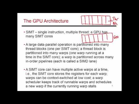
The GPU, a High Level View at the Hardware
We can see the GPU like a collection of processors, sharing some common memory, akin to a traditional multi-processor system. Each processor executes code independently of the others, and internally it has tens to hundreds of cores, and some private memory space; in some GPUs the different processors can even execute different programs. The cores are often grouped in groups, and each group executes the same code, instruction by instruction, in the same order and at the same time. All cores have access to the processor’s private memory space.
How Programs are Executed
Let us assume we are sending our code to the GPU for execution; how is the code being executed by the different processors? First of all, we need to know that each processor will execute the same code. As an example, we can look back at some code that we executed on the GPU using Numba, like the following snippet.
PYTHON
import numba as nb

@nb.vectorize(['int32(int32)'], target='cuda')
def check_prime_gpu(num):
    for i in range(2, (num // 2) + 1):
       if (num % i) == 0:
           return 0
    return num
We did not need to write a different check_prime_gpu
function for each processor, or core, on the GPU; actually, we have no
idea how many processors and cores are available on the GPU we just used
to execute this code!
So we can imagine that each processors receives its copy of the
check_prime_gpu function, and executes it independently of
the other processors. We also know that by executing the following
Python snippet, we are telling the GPU to execute our function on all
numbers between 0 and 100000.
So each processor will get a copy of the code, and one subset of the numbers between 0 and 10000. If we assume that our GPU has 4 processors, each of them will get around 2500 numbers to process; the processing of these numbers will be split among the various cores that the processor has. Again, let us assume that each processor has 8 cores, divided in 2 groups of 4 cores. Therefore, the 2500 numbers to process will be divided inside the processors in sets of 4 elements, and these sets will be scheduled for execution on the 2 groups of cores that each processor has available. While the processors cannot communicate with each other, the cores of the same processor can; however, there is no communication in our example code.
While so far in the lesson we had no control over the way in which the computation is mapped to the GPU for execution, this is something that we will address soon.
Different Memories
Another detail that we need to understand is that GPUs have different memories. We have a main memory that is available to all processors on the GPU; this memory, as we already know, is often physically separate from the CPU memory, but copies to and from are possible. Using this memory we can send data to the GPU, and copy results back to the CPU. This memory is not coherent, meaning that there is no guarantee that code running on one GPU processor will see the results of code running on a different GPU processor.
Internally, each processor has its own memory. This memory is faster than the GPU main memory, but smaller in size, and it is also coherent, although we need to wait for all cores to finish their memory operations before the results produced by some cores are available to all other cores in the same processor. Therefore, this memory can be used for communication among cores.
Finally, each core has also a very small, but very fast, memory, that is used mainly to store the operands of the instructions executed by each core. This memory is private, and cannot generally be used for communication.
Content from Your First GPU Kernel
Last updated on 2026-06-02 | Edit this page
Overview
Questions
- “How do I identify data parallelism in my code?”
- “How do I write a GPU program?”
- “What is CUDA?”
- “How are CUDA threads organised into blocks and grids?”
Objectives
- “Recognize possible data parallelism in Python code”
- “Describe the role of the
__global__,__host__, and__device__keywords in a CUDA program” - “Use
threadIdx,blockIdx, andblockDimto compute the global index of a thread” - “Write a CUDA kernel that handles input arrays of arbitrary size”
- “Execute a CUDA program in Python and measure its execution time”
Summing Two Vectors in Python
We start by introducing a program that, given two input vectors of the same size, stores the sum of the corresponding elements of the two input vectors into a third one.
One of the characteristics of this program is that each iteration of
the for loop is independent of the other iterations. In
other words, we could reorder the iterations and still produce the same
output, or even compute each iteration in parallel or on a different
device, and still come up with the same output. These are the kind of
programs that we would call naturally parallel, and they are
perfect candidates for being executed on a GPU.
Summing Two Vectors in CUDA
While we could just use CuPy to run something equivalent to our
vector_add on a GPU, our goal is to learn how to write code
that can be executed by GPUs, therefore we now begin learning CUDA.
The CUDA-C language is a GPU programming language and API developed by NVIDIA. It is mostly equivalent to C/C++, with some special keywords, built-in variables, and functions.
We begin our introduction to CUDA by writing a small kernel, i.e. a GPU program, that computes the same function that we just described in Python.
C
extern "C"
__global__ void vector_add(const float * A, const float * B, float * C, const int size)
{
int item = threadIdx.x;
C[item] = A[item] + B[item];
}We are aware that CUDA is a proprietary solution, and that there are more open and portable solutions, however CUDA is also the most used platform for GPU programming and therefore we decided to use it for our teaching material. Nevertheless, almost everything we cover in this lesson does also apply to HIP, a portable language that can run on both NVIDIA and AMD GPUs.
Running Code on the GPU
Before delving deeper into the meaning of all lines of code, and before starting to understand how CUDA works, let us execute the code on a GPU and check if it is correct or not. To compile the code and manage the GPU in Python we are going to use the interface provided by NVIDIA.
PYTHON
import cupy as cp
from cuda.core import Device, LaunchConfig, Program, ProgramOptions, launch
# initialize the GPU
gpu = Device()
gpu.set_current()
stream = gpu.create_stream()
program_options = ProgramOptions(std="c++17", arch=f"sm_{gpu.arch}")
# size of the vectors
size = 1024
# allocating and populating the vectors on the GPU
a_gpu = cp.random.rand(size, dtype=cp.float32)
b_gpu = cp.random.rand(size, dtype=cp.float32)
c_gpu = cp.zeros(size, dtype=cp.float32)
# CUDA vector_add source code
vector_add_cuda_code = r'''
extern "C"
__global__ void vector_add(const float * A, const float * B, float * C, const int size)
{
int item = threadIdx.x;
C[item] = A[item] + B[item];
}
'''
# compiling the CUDA code
prog = Program(vector_add_cuda_code, code_type="c++", options=program_options)
mod = prog.compile("cubin", name_expressions=("vector_add",))
vector_add_gpu = mod.get_kernel("vector_add")
# execute the code on the GPU
config = LaunchConfig(grid=(1, 1, 1), block=(size, 1, 1))
launch(stream, config, vector_add_gpu, a_gpu.data.ptr, b_gpu.data.ptr, c_gpu.data.ptr, size)And to be sure that the CUDA code does exactly what we want, we can execute our sequential Python code and compare the results.
PYTHON
import numpy as np
a_cpu = cp.asnumpy(a_gpu)
b_cpu = cp.asnumpy(b_gpu)
c_cpu = np.zeros(size, dtype=np.float32)
vector_add(a_cpu, b_cpu, c_cpu, size)
# test
if np.allclose(c_cpu, c_gpu):
print("Correct results!")OUTPUT
Correct results!Understanding the CUDA Code
We can now move back to the CUDA code and analyze it line by line to highlight the differences between CUDA-C and standard C.
This is the definition of our CUDA vector_add function.
The __global__ keyword is an execution space identifier,
and it is specific to CUDA. What this keyword means is that the defined
function will be able to run on the GPU, but can also be called from the
host (in our case the Python interpreter running on the CPU). All of our
kernel definitions will be preceded by this keyword.
Other execution space identifiers in CUDA-C are
__host__, and __device__. Functions annotated
with the __host__ identifier will run on the host, and be
only callable from the host, while functions annotated with the
__device__ identifier will run on the GPU, but can only be
called from the GPU itself. We are not going to use these identifiers as
often as __global__.
The following table offers a recapitulation of the keywords we just introduced.
| Keyword | Description |
|---|---|
__global__ |
the function is visible to the host and the GPU, and runs on the GPU |
__host__ |
the function is visible only to the host, and runs on the host |
__device__ |
the function is visible only to the GPU, and runs on the GPU |
The following is the part of the code in which we do the actual work.
As you may see, it looks similar to the innermost loop of our
vector_add Python function, with the main difference being
in how the value of the item variable is evaluated.
In fact, while in Python the content of item is the
result of the range function, in CUDA we are reading a
special variable, i.e. threadIdx, containing a triplet that
indicates the id of a thread inside a three-dimensional CUDA block. In
this particular case we are working on a one dimensional vector, and
therefore only interested in the first dimension, that is stored in the
x field of this variable.
Challenge: loose threads
We know enough now to pause for a moment and do a little exercise.
Assume that in our vector_add kernel we replace the
following line:
With this other line of code:
What will the result of this change be?
- Nothing changes
- Only the first thread is working
- Only
C[1]is written - All elements of
Care zero
The correct answer is number 3, only the element C[1] is
written, and we do not even know by which thread!
Computing Hierarchy in CUDA
In the previous example we had a small vector of size 1024, and each of the 1024 threads we generated was working on one of the elements.
What would happen if we changed the size of the vector to a larger number, such as 2048? We modify the value of the variable size and try again.
PYTHON
# size of the vectors
size = 2048
# allocating and populating the vectors
a_gpu = cp.random.rand(size, dtype=cp.float32)
b_gpu = cp.random.rand(size, dtype=cp.float32)
c_gpu = cp.zeros(size, dtype=cp.float32)
config = LaunchConfig(grid=(1, 1, 1), block=(size, 1, 1))
launch(stream, config, vector_add_gpu, a_gpu.data.ptr, b_gpu.data.ptr, c_gpu.data.ptr, size)This is how the output should look when running the code in a Jupyter Notebook:
OUTPUT
---------------------------------------------------------------------------
CUDAError Traceback (most recent call last)
/tmp/ipython-input-2754325452.py in <cell line: 0>()
8
9 config = LaunchConfig(grid=(1, 1, 1), block=(size, 1, 1))
---> 10 launch(stream, config, vector_add_gpu, a_gpu.data.ptr, b_gpu.data.ptr, c_gpu.data.ptr, size)
cuda/core/_launcher.pyx in cuda.core._launcher.launch()
cuda/core/_utils/cuda_utils.pyx in cuda.core._utils.cuda_utils.HANDLE_RETURN()
cuda/core/_utils/cuda_utils.pyx in cuda.core._utils.cuda_utils._check_driver_error()
CUDAError: CUDA_ERROR_INVALID_VALUE: This indicates that one or more of the parameters passed to the API call is not within an acceptable range of values.The reason for this error is that most GPUs will not allow us to
execute a block composed of more than 1024 threads. If we look at the
launch config of our function we see that the block and
grid parameters are two triplets.
The first triplet specifies the size of the CUDA
grid, while the second triplet specifies the size of
the CUDA block. The grid is a three-dimensional
structure in the CUDA programming model and it represents the
organization of a whole kernel execution. A grid is made of one or more
independent blocks, and in the case of our previous snippet of code we
have a grid composed by a single block (1, 1, 1). The size
of this block is specified by the second triplet, in our case
(size, 1, 1). While blocks are independent of each other,
the threads composing a block are not completely independent, they share
resources and can also communicate with each other.
To go back to our example, we can modify the grid specification from
(1, 1, 1) to (2, 1, 1), and the block
specification from (size, 1, 1) to
(size // 2, 1, 1).
If we run the code again, the error should be now gone.
We already introduced the special variable threadIdx
when introducing the vector_add CUDA code, and we said it
contains a triplet specifying the coordinates of a thread in a thread
block. CUDA has other variables that are important to understand the
coordinates of each thread and block in the overall structure of the
computation.
These special variables are blockDim,
blockIdx, and gridDim, and they are all
triplets. The triplet contained in blockDim represents the
size of the calling thread’s block in three dimensions. While the
content of threadIdx is different for each thread in the
same block, the content of blockDim is the same because the
size of the block is the same for all threads. The coordinates of a
block in the computational grid are contained in blockIdx,
therefore the content of this variable will be the same for all threads
in the same block, but different for threads in different blocks.
Finally, gridDim contains the size of the grid in three
dimensions, and it is again the same for all threads.
The following table offers a recapitulation of the keywords we just introduced.
| Keyword | Description |
|---|---|
threadIdx |
the ID of a thread in a block |
blockDim |
the size of a block, i.e. the number of threads per dimension |
blockIdx |
the ID of a block in the grid |
gridDim |
the size of the grid, i.e. the number of blocks per dimension |
The content of blockDim is (512, 1, 1) and
the content of gridDim is (4, 1, 1), for all
threads.
What happens if we then run the code that we just modified to work on a vector of 2048 elements, and compare the results with our CPU version?
PYTHON
# reallocate the CPU arrays
a_cpu = cp.asnumpy(a_gpu)
b_cpu = cp.asnumpy(b_gpu)
c_cpu = np.zeros(size, dtype=np.float32)
# CPU code
vector_add(a_cpu, b_cpu, c_cpu, size)
# GPU code
launch(stream, config, vector_add_gpu, a_gpu.data.ptr, b_gpu.data.ptr, c_gpu.data.ptr, size)
# test
if np.allclose(c_cpu, c_gpu):
print("Correct results!")
else:
print("Wrong results!")OUTPUT
Wrong results!The results are wrong! In fact, while we increased the number of threads we launch, we did not modify the kernel code to compute the correct results using the new builtin variables we just introduced.
Challenge: scaling up
The correct answer is
(blockIdx.x * blockDim.x) + threadIdx.x. The following code
is the complete vector_add that can work with vectors
larger than 1024 elements.
Vectors of Arbitrary Size
So far we have worked with a number of threads that is the same as the elements in the vector. However, in a real world scenario we may have to process vectors of arbitrary size, and to do this we need to modify both the kernel and the way it is launched.
Challenge: more work than necessary
We modified the vector_add kernel to include a check for
the size of the vector, so that we only compute elements that are within
the vector boundaries. However the code is not correct as it is written
now. Can you rewrite the code to make it work?
The correct way to modify the vector_add to work on
vectors of arbitrary size is to first compute the coordinates of each
thread, and then perform the sum only on elements that are within the
vector boundaries, as shown in the following snippet of code.
To test our changes we can modify the size of the
vectors from 2048 to 10000, and execute the code again.
PYTHON
size = 10_000
# reallocating and populating the vectors
a_gpu = cp.random.rand(size, dtype=cp.float32)
b_gpu = cp.random.rand(size, dtype=cp.float32)
c_gpu = cp.zeros(size, dtype=cp.float32)
# recompiling the CUDA code
prog = Program(vector_add_cuda_code, code_type="c++", options=program_options)
mod = prog.compile("cubin", name_expressions=("vector_add",))
vector_add_gpu = mod.get_kernel("vector_add")OUTPUT
---------------------------------------------------------------------------
CUDAError Traceback (most recent call last)
/tmp/ipython-input-2155189089.py in <cell line: 0>()
11 vector_add_gpu = mod.get_kernel("vector_add")
12
---> 13 launch(stream, config, vector_add_gpu, a_gpu.data.ptr, b_gpu.data.ptr, c_gpu.data.ptr, size)
cuda/core/_launcher.pyx in cuda.core._launcher.launch()
cuda/core/_utils/cuda_utils.pyx in cuda.core._utils.cuda_utils.HANDLE_RETURN()
cuda/core/_utils/cuda_utils.pyx in cuda.core._utils.cuda_utils._check_driver_error()
CUDAError: CUDA_ERROR_INVALID_VALUE: This indicates that one or more of the parameters passed to the API call is not within an acceptable range of values.This error is telling us that CUDA cannot launch a block with
size // 2 threads, because the maximum amount of threads in
a kernel is 1024 and we are requesting 5000 threads.
What we need to do is to make grid and block more flexible, so that
they can adapt to vectors of arbitrary size. To do that, we can replace
the Python code to call vector_add_gpu with the following
code.
PYTHON
import math
grid_size = (int(math.ceil(size / 1024)), 1, 1)
block_size = (1024, 1, 1)
config = LaunchConfig(grid=grid_size, block=block_size)
launch(stream, config, vector_add_gpu, a_gpu.data.ptr, b_gpu.data.ptr, c_gpu.data.ptr, size)With these changes we always have blocks composed of 1024 threads, but we adapt the number of blocks so that we always have enough threads to compute all elements in the vector. If we want to be able to easily modify the number of threads per block, we can even rewrite the code like the following:
PYTHON
threads_per_block = 1024
grid_size = (int(math.ceil(size / threads_per_block)), 1, 1)
block_size = (threads_per_block, 1, 1)
config = LaunchConfig(grid=grid_size, block=block_size)
launch(stream, config, vector_add_gpu, a_gpu.data.ptr, b_gpu.data.ptr, c_gpu.data.ptr, size)So putting this all together in a full snippet, we can execute the working code and get the correct output.
PYTHON
import math
import numpy as np
import cupy as cp
from cuda.core import Device, LaunchConfig, Program, ProgramOptions, launch
# Size of the vectors
size = 10_000_000
# Python vector add
def vector_add(A, B, C, size):
    for item in range(0, size):
        C[item] = A[item] + B[item]
# Initialize the GPU
gpu = Device()
gpu.set_current()
stream = gpu.create_stream()
program_options = ProgramOptions(std="c++17", arch=f"sm_{gpu.arch}")
# Allocate and populate the vectors on the GPU
a_gpu = cp.random.rand(size, dtype=cp.float32)
b_gpu = cp.random.rand(size, dtype=cp.float32)
c_gpu = cp.zeros(size, dtype=cp.float32)
# Allocate the CPU arrays
a_cpu = cp.asnumpy(a_gpu)
b_cpu = cp.asnumpy(b_gpu)
c_cpu = np.zeros(size, dtype=np.float32)
# CUDA vector_add source code
vector_add_cuda_code = r'''
extern "C"
__global__ void vector_add(const float * A, const float * B, float * C, const int size)
{
int item = (blockIdx.x * blockDim.x) + threadIdx.x;
if (item < size) {
C[item] = A[item] + B[item];
}
}
'''
# Execute the CPU code
%timeit -n 1 -r 1 vector_add(a_cpu, b_cpu, c_cpu, size)
# Compile the CUDA code
prog = Program(vector_add_cuda_code, code_type="c++", options=program_options)
mod = prog.compile("cubin", name_expressions=("vector_add",))
vector_add_gpu = mod.get_kernel("vector_add")
# Execute the code on the GPU
threads_per_block = 1024
grid_size = (int(math.ceil(size / threads_per_block)), 1, 1)
block_size = (threads_per_block, 1, 1)
config = LaunchConfig(grid=grid_size, block=block_size)
%timeit launch(stream, config, vector_add_gpu, a_gpu.data.ptr, b_gpu.data.ptr, c_gpu.data.ptr, size); stream.sync()
# Test
if np.allclose(c_cpu, c_gpu):
print("Correct results!")
else:
print("Wrong results!")OUTPUT
Correct results!Challenge: compute prime numbers with CUDA
Given the following Python code, similar to what we have seen in the previous episode about Numba, write the missing CUDA kernel that computes all the prime numbers up to a certain upper bound.
PYTHON
import math
import numpy as np
import cupy as cp
from cuda.core import Device, LaunchConfig, Program, ProgramOptions, launch
# Initialize the GPU
gpu = Device()
gpu.set_current()
stream = gpu.create_stream()
program_options = ProgramOptions(std="c++17", arch=f"sm_{gpu.arch}")
# CPU version
def all_primes_to(upper : int, prime_list : list):
for num in range(0, upper):
prime = True
for i in range(2, (num // 2) + 1):
if (num % i) == 0:
prime = False
break
if prime:
prime_list[num] = 1
upper_bound = 100_000
all_primes_cpu = np.zeros(upper_bound, dtype=np.int32)
# GPU version
check_prime_gpu_code = r'''
extern "C"
__global__ void all_primes_to(int size, int * const all_prime_numbers)
{
for ( int number = 0; number < size; number++ )
{
int result = 1;
for ( int factor = 2; factor <= number / 2; factor++ )
{
if ( number % factor == 0 )
{
result = 0;
break;
}
}
all_prime_numbers[number] = result;
}
}
'''
# Allocate memory
all_primes_gpu = cp.zeros(upper_bound, dtype=cp.int32)
# Compile the CUDA code
prog = Program(check_prime_gpu_code, code_type="c++", options=program_options)
mod = prog.compile("cubin", name_expressions=("all_primes_to",))
all_primes_to_gpu = mod.get_kernel("all_primes_to")
# Setup the grid
grid_size = (int(math.ceil(upper_bound / 1024)), 1, 1)
block_size = (1024, 1, 1)
config = LaunchConfig(grid=grid_size, block=block_size)
# Benchmark and test
%timeit -n 1 -r 1 all_primes_to(upper_bound, all_primes_cpu)
%timeit launch(stream, config, all_primes_to_gpu, upper_bound, all_primes_gpu.data.ptr); stream.sync()
if np.allclose(all_primes_cpu, all_primes_gpu):
print("Correct results!")
else:
print("Wrong results!")There is no need to modify anything in the code, except the body of
the CUDA all_primes_to inside the
check_prime_gpu_code string, as we did in the examples so
far.
Be aware that the provided CUDA code is a direct port of the Python
code, and therefore very slow. If you want to test it, use a lower value
for upper_bound.
One possible solution for the CUDA kernel is provided in the following code.
C
extern "C"
__global__ void all_primes_to(int size, int * const all_prime_numbers)
{
int number = (blockIdx.x * blockDim.x) + threadIdx.x;
int result = 1;
if ( number < size )
{
for ( int factor = 2; factor <= number / 2; factor++ )
{
if ( number % factor == 0 )
{
result = 0;
break;
}
}
all_prime_numbers[number] = result;
}
}The outermost loop in Python is replaced by having each thread testing for primeness a different number of the sequence. Having one number assigned to each thread via its ID, the kernel implements the innermost loop the same way it is implemented in Python.
- “Precede your kernel definition with the
__global__keyword” - “Use built-in variables
threadIdx,blockIdx,gridDimandblockDimto identify each thread” - “The global index of a thread is
(blockIdx.x * blockDim.x) + threadIdx.x” - “Add a bounds check (
if (item < size)) in your kernel when the total number of threads may exceed the input size”
Content from Registers, Global, and Local Memory
Last updated on 2026-06-02 | Edit this page
Overview
Questions
- “What are registers?”
- “How do I share data between host and GPU?”
- “What are the differences between the memory spaces available in CUDA?”
- “What happens when a thread uses more variables than there are available registers?”
Objectives
- “Describe the scope, lifetime, and performance characteristics of registers, global memory, and local memory”
- “Identify which memory type is used for a given variable in a CUDA kernel”
- “Explain when the compiler automatically uses local memory instead of registers”
Now that we know how to write a CUDA kernel to run code on the GPU, and how to use the Python interface provided by CuPy to execute it, it is time to look at the different memory spaces in the CUDA programming model.
Registers
Registers are fast on-chip memories that are used to store operands for the operations executed by the computing cores.
Did we encounter registers in the vector_add code used
in the previous episode? Yes we did! The variable item is,
in fact, stored in a register for at least part, if not all, of a
thread’s execution. In general all scalar variables defined in CUDA code
are stored in registers.
Registers are local to a thread, and each thread has exclusive access to its own registers: values in registers cannot be accessed by other threads, even from the same block, and are not available for the host. Registers are also not permanent, therefore data stored in registers is only available during the execution of a thread.
Challenge: how many registers are we using?
In general, it is not possible to exactly know how many registers the
compiler will use without examining the output generated by the compiler
itself. However, we can roughly estimate the amount of necessary
registers based on the variables used. We most probably need one
register to store the variable item, two registers to store
the content of A[item] and B[item], and one
additional register to store the sum A[item] + B[item]. So
the number of registers that vector_add probably uses is
4.
If we want to make registers use more explicit in the
vector_add code, we can try to rewrite it in a slightly
different, but equivalent, way.
C
extern "C"
__global__ void vector_add(const float * A, const float * B, float * C, const int size)
{
int item = (blockIdx.x * blockDim.x) + threadIdx.x;
float temp_a, temp_b, temp_c;
if ( item < size )
{
temp_a = A[item];
temp_b = B[item];
temp_c = temp_a + temp_b;
C[item] = temp_c;
}
}In this new version of vector_add we explicitly declare
three float variables to store the values loaded from
memory and the sum of our input items, making the estimation of used
registers more obvious.
This is totally unnecessary in the case of our example, because the compiler will determine on its own the right amount of registers to allocate per thread, and what to store in them. However, explicit register usage can be important for reusing items already loaded from memory.
Registers are the fastest memory on the GPU, so using them to increase data reuse is an important performance optimization. We will look at some examples of manually using registers to improve performance in future episodes.
Small CUDA arrays, whose size is known at compile time, will also be
allocated in registers by the compiler. We can rewrite the previous
version of vector_add to work with an array of
registers.
C
extern "C"
__global__ void vector_add(const float * A, const float * B, float * C, const int size)
{
int item = (blockIdx.x * blockDim.x) + threadIdx.x;
float temp[3];
if ( item < size )
{
temp[0] = A[item];
temp[1] = B[item];
temp[2] = temp[0] + temp[1];
C[item] = temp[2];
}
}Once again, this is not something that we would normally do, and it is provided only as an example of how to work with arrays of registers.
Global Memory
Global memory can be considered the main memory space of the GPU in CUDA. It is allocated, and managed, by the host, and it is accessible to both the host and the GPU, and for this reason the global memory space can be used to exchange data between the two. It is the largest memory space available, and therefore it can contain much more data than registers, but it is also slower to access. This memory space does not require any special memory space identifier.
Challenge: identify when global memory is used
The vectors A, B, and C are
stored in global memory.
Memory allocated on the host, and passed as a parameter to a kernel, is by default allocated in global memory.
Global memory is accessible by all threads, from all thread blocks. This means that a thread can read and write any value in global memory.
While global memory is visible to all threads, remember that global memory is not coherent, and changes made by one thread block may not be available to other thread blocks during the kernel execution. However, all memory operations are finalized when the kernel terminates.
Local Memory
Memory can also be statically allocated from within a kernel, and according to the CUDA programming model such memory will not be global but local memory. Local memory is only visible, and therefore accessible, by the thread allocating it. So all threads executing a kernel will have their own privately allocated local memory.
Challenge: use local memory
Modify the following version of vector_add so that
intermediate data products are stored in local memory, and only the
final result is saved into global memory.
C
extern "C"
__global__ void vector_add(const float * A, const float * B, float * C, const int size)
{
   int item = (blockIdx.x * blockDim.x) + threadIdx.x;
   if ( item < size )
   {
      C[item] = A[item] + B[item];
   }
}Hint: have a look at the example using an array of registers, but find a way to use a variable and not a constant for the size.
We need to pass the size of the local array as a new parameter to the
kernel, because if we just specified 3 in the code, the
compiler would allocate registers and not local memory.
C
extern "C"
__global__ void vector_add(const float * A, const float * B, float * C, const int size, const int local_memory_size)
{
int item = (blockIdx.x * blockDim.x) + threadIdx.x;
float local_memory[local_memory_size];
if ( item < size )
{
local_memory[0] = A[item];
local_memory[1] = B[item];
local_memory[2] = local_memory[0] + local_memory[1];
C[item] = local_memory[2];
}
}The host code could be modified by adding one line and changing the way the kernel is called.
Local memory is not a particularly fast memory, and in fact it has similar throughput and latency of global memory, but it is much larger than registers. As an example, local memory is automatically used by the CUDA compiler to store spilled registers, i.e. to temporarily store variables that cannot be kept in registers anymore because there is not enough space in the register file, but that will be used again in the future and so cannot be erased.
- “Registers are the fastest GPU memory; use them to store intermediate values and avoid repeated reads from global memory”
- “Global memory is the main memory space and it is used to share data between host and GPU”
- “Local memory is private to each thread and has similar latency to global memory; the compiler uses it automatically when a thread runs out of registers”
Content from Constant Memory
Last updated on 2026-06-02 | Edit this page
Overview
Questions
- “Is there a way to have a read-only cache in CUDA?”
Objectives
- “Understanding when and how to use constant memory”
Constant Memory
Constant memory is a read-only cache whose content can be broadcast
to multiple threads in a block. A variable allocated in constant memory
needs to be declared in CUDA by using the special
__constant__ identifier, and it must be a global variable,
i.e. it must be declared in the scope that contains the kernel, not
inside the kernel itself. If all of this sounds complex do not worry, we
are going to see how this works with an example.
C
extern "C" {
#define BLOCKS 2
__constant__ float factors[BLOCKS];
__global__ void sum_and_multiply(const float * A, const float * B, float * C, const int size)
{
int item = (blockIdx.x * blockDim.x) + threadIdx.x;
C[item] = (A[item] + B[item]) * factors[blockIdx.x];
}
}In the previous code snippet we implemented a kernel that, given two
vectors A and B, stores their element-wise sum
in a third vector, C, scaled by a certain factor; this
factor is the same for all threads in the same thread block. Because
these factors are shared, i.e. all threads in the same thread block use
the same factor for scaling their sums, it is a good idea to use
constant memory for the factors array. In fact you can see
that the definition of factors is preceded by the
__constant__ keyword, and said definition is in the global
scope. It is important to note that the size of the constant array needs
to be known at compile time, therefore the use of the
#define preprocessor statement. On the kernel side there is
no need to do more, the factors vector can be normally
accessed inside the code as any other vector, and because it is a global
variable it does not need to be passed to the kernel as a function
argument.
The initialization of constant memory happens on the host side, and we show how this is done in the next code snippet.
PYTHON
# TODO: the code does not work with cuda.core
# Compile the code
mod = prog.compile("cubin", name_expressions=("sum_and_multiply",))
# Allocate and copy constant memory
factors_ptr = mod.get_global("factors")
factors_gpu = cp.ndarray(2, cp.float32, factors_ptr)
factors_gpu[...] = cp.random.random(2, dtype=cp.float32)From the previous code it is clear that dealing with constant memory
is a slightly more verbose affair than usual. First, we need to compile
the code, that in this case is contained in a Python string named
cuda_code. This is necessary because constant memory is
defined in the CUDA code, so we need CUDA to allocate the necessary
memory, and then provide us with a pointer to this memory. By calling
the method get_global we ask the CUDA subsystem to provide
us with the location of a global object, in this case the array
factors. We can then create our own CuPy array and point
that to the object returned by get_global, so that we can
use it in Python as we would normally do. Note that we use the constant
2 for the size of the array, the same number we are using
in the CUDA code; it is important that we use the same number or we may
end up accessing memory that is outside the bounds of the array. Lastly,
we initialize the array with some random floating point numbers.
In our case the output of this line of code is two floating point
numbers, e.g. [0.11390183 0.2585096 ]. However, we are not
really accessing the content of the GPU’s constant memory from the host,
we are simply accessing the host-side copy of the data maintained by
CuPy.
We can now combine all the code together and execute it.
PYTHON
import math
import numpy as np
import cupy as cp
from cuda.core import Device, LaunchConfig, Program, ProgramOptions, launch
# Initialize the GPU
gpu = Device()
gpu.set_current()
stream = gpu.create_stream()
program_options = ProgramOptions(std="c++17", arch=f"sm_{gpu.arch}")
# Size of the vectors
size = 2048
# Allocating and populating the vectors
a_gpu = cp.random.rand(size, dtype=cp.float32)
b_gpu = cp.random.rand(size, dtype=cp.float32)
c_gpu = cp.zeros(size, dtype=cp.float32)
# CUDA code
cuda_code = r'''
extern "C" {
#define BLOCKS 2
__constant__ float factors[BLOCKS];
__global__ void sum_and_multiply(const float * A, const float * B, float * C, const int size)
{
int item = (blockIdx.x * blockDim.x) + threadIdx.x;
C[item] = (A[item] + B[item]) * factors[blockIdx.x];
}
}
'''
# Compile and access the code
prog = Program(cuda_code, code_type="c++", options=program_options)
mod = prog.compile("cubin", name_expressions=("sum_and_multiply",))
sum_and_multiply = mod.get_kernel("sum_and_multiply")
threads_per_block = 1024
grid_size = (int(math.ceil(size / threads_per_block)), 1, 1)
block_size = (threads_per_block, 1, 1)
config = LaunchConfig(grid=grid_size, block=block_size)
# Allocate and copy constant memory
# TODO: cuda.core does not expose constant memory, cuda.bindings should be used instead
# The episode will be updated in the future
factors_ptr = mod.get_global("factors")
factors_gpu = cp.ndarray(2, cp.float32, factors_ptr)
factors_gpu[...] = cp.random.random(2, dtype=cp.float32)
launch(stream, config, sum_and_multiply, a_gpu.data.ptr, b_gpu.data.ptr, c_gpu.data.ptr, size)As you can see the code is not very general, it uses constants and works only with two blocks, but it is a working example of how to use constant memory.
Challenge: generalize the previous code
Have a look again at the code using constant memory, and make it general enough to be able to run on input of arbitrary size. Experiment with some different input sizes.
One of the possible solutions is the following one.
PYTHON
# size of the vectors
size = 10**6
# allocating and populating the vectors
a_gpu = cp.random.rand(size, dtype=cp.float32)
b_gpu = cp.random.rand(size, dtype=cp.float32)
c_gpu = cp.zeros(size, dtype=cp.float32)
# prepare arguments
args = (a_gpu, b_gpu, c_gpu, size)
# CUDA code
cuda_code = r'''
extern "C" {
__constant__ float factors[BLOCKS];
__global__ void sum_and_multiply(const float * A, const float * B, float * C, const int size)
{
int item = (blockIdx.x * blockDim.x) + threadIdx.x;
if ( item < size )
{
C[item] = (A[item] + B[item]) * factors[blockIdx.x];
}
}
}
'''
# compute the number of blocks and replace "BLOCKS" in the CUDA code
threads_per_block = 1024
num_blocks = int(math.ceil(size / threads_per_block))
cuda_code = cuda_code.replace("BLOCKS", f"{num_blocks}")
# compile and access the code
module = cp.RawModule(code=cuda_code)
sum_and_multiply = module.get_function("sum_and_multiply")
# allocate and copy constant memory
factors_ptr = module.get_global("factors")
factors_gpu = cp.ndarray(num_blocks, cp.float32, factors_ptr)
factors_gpu[...] = cp.random.random(num_blocks, dtype=cp.float32)
sum_and_multiply((num_blocks, 1, 1), (threads_per_block, 1, 1), args)- “Globally scoped arrays, whose size is known at compile time, can be
stored in constant memory using the
__constant__identifier”
Content from Concurrent access to the GPU
Last updated on 2026-06-02 | Edit this page
Overview
Questions
- “Is it possible to concurrently execute more than one kernel on a single GPU?”
Objectives
- “Understand how to use CUDA streams and events”
Concurrently execute two kernels on the same GPU
So far we only focused on completing one operation at a time on the GPU, writing and executing a single CUDA kernel each time. However the GPU has enough resources to perform more than one task at the same time.
Let us assume that, for our program, we need to compute both a list of prime numbers, and a histogram, two kernels that we developed in this same lesson. We could write both kernels in CUDA, and then execute them on the GPU, as shown in the following code.
PYTHON
import numpy as np
import cupy as cp
import math
from cuda.core import Device, LaunchConfig, Program, ProgramOptions, launch
upper_bound = 100_000
histogram_size = 2**25
# Initialize the GPU
gpu = Device()
gpu.set_current()
stream = gpu.create_stream()
program_options = ProgramOptions(std="c++17", arch=f"sm_{gpu.arch}")
# GPU code
check_prime_gpu_code = r'''
extern "C"
__global__ void all_primes_to(int size, int * const all_prime_numbers)
{
    int number = (blockIdx.x * blockDim.x) + threadIdx.x;
    int result = 1;

    if ( number < size )
    {
        for ( int factor = 2; factor <= number / 2; factor++ )
        {
            if ( number % factor == 0 )
            {
                result = 0;
                break;
            }
        }

        all_prime_numbers[number] = result;
    }
}
'''
histogram_cuda_code = r'''
extern "C"
__global__ void histogram(const int * input, int * output)
{
int item = (blockIdx.x * blockDim.x) + threadIdx.x;
__shared__ int temp_histogram[256];
// Initialize shared memory and synchronize
temp_histogram[threadIdx.x] = 0;
__syncthreads();
// Compute shared memory histogram and synchronize
atomicAdd(&(temp_histogram[input[item]]), 1);
__syncthreads();
// Update global histogram
atomicAdd(&(output[threadIdx.x]), temp_histogram[threadIdx.x]);
}
'''
# Allocate memory
all_primes_gpu = cp.zeros(upper_bound, dtype=cp.int32)
input_gpu = cp.random.randint(256, size=histogram_size, dtype=cp.int32)
output_gpu = cp.zeros(256, dtype=cp.int32)
# Compile and setup the grid for all_primes_to
prog = Program(check_prime_gpu_code, code_type="c++", options=program_options)
mod = prog.compile("cubin", name_expressions=("all_primes_to",))
all_primes_to_gpu = mod.get_kernel("all_primes_to")
grid_size = (int(math.ceil(upper_bound / 1024)), 1, 1)
block_size = (1024, 1, 1)
config_primes = LaunchConfig(grid=grid_size, block=block_size)
# Compile and setup the grid for histogram
prog = Program(histogram_cuda_code, code_type="c++", options=program_options)
mod = prog.compile("cubin", name_expressions=("histogram",))
histogram_gpu = mod.get_kernel("histogram")
grid_size = (int(math.ceil(histogram_size / 256)), 1, 1)
block_size = (256, 1, 1)
config_histogram = LaunchConfig(grid=grid_size, block=block_size)
# Execute the kernels
launch(stream, config_primes, all_primes_to_gpu, upper_bound, all_primes_gpu.data.ptr)
launch(stream, config_histogram, histogram_gpu, input_gpu.data.ptr, output_gpu.data.ptr)
stream.sync()
# Save results to do something else later
output_one = all_primes_gpu
output_two = output_gpuIn the previous code, after allocating memory and compiling, we execute and measure the performance of one kernel, and when we are done we do the same for the other kernel.
This is technically correct, but there is no reason why one kernel should be executed before the other, because there is no dependency between these two operations.
Therefore, while this is fine in our example, in a real application we may want to run the two kernels concurrently on the GPU to reduce the total execution time. To achieve this in CUDA we need to use CUDA streams.
A stream is a sequence of GPU operations that is executed in order, and so far we have been implicitly using the default stream. This is the reason why all the operations we issued, such as data transfers and kernel invocations, are performed in the order we specify them in the Python code, and not in any other.
Have you wondered why after requesting data transfers to and from the GPU, we do not stop to check if they are complete before performing operations on such data? The reason is that within a stream all operations are carried out in order, so the kernel calls in our code are always performed after the data transfer from host to device is complete, and so on.
If we want to create new CUDA streams, we can do it in the following way.
We can then execute the kernels in different streams by passing the
stream object to the launch function.
PYTHON
launch(stream_one, config_primes, all_primes_to_gpu, upper_bound, all_primes_gpu.data.ptr)
launch(stream_two, config_histogram, histogram_gpu, input_gpu.data.ptr, output_gpu.data.ptr)The result of doing this is that the second kernel,
i.e. histogram_gpu, does not need to wait for
all_primes_to_gpu to finish before being executed.
Stream synchronization
If we need to wait for all operations on a certain stream to finish,
we can call the sync method. Continuing with the previous
example, in the following Python snippet we wait for the execution of
all_primes_to_gpu on stream_one to finish.
This synchronization primitive is useful when we need to be sure that
all operations on a stream are finished, before continuing. It is,
however, a bit coarse grained. Imagine having a stream with a whole
sequence of operations enqueued, and another stream with one data
dependency on one of these operations. If we use sync, we
wait until all operations of said stream are completed before executing
the other stream, thus negating the whole reason of using streams in the
first place.
A possible solution is to insert a CUDA event at a certain position in the stream, and then wait specifically for that event. Events are created in Python in the following way.
And can then be added to a stream by using the record
method. In the following example we will create two streams: in the
first we will execute all_primes_to_gpu twice, while in the
second one we will execute histogram_gpu with the condition
that the kernel in the second stream is executed only after the first
prime number computation is complete.
PYTHON
stream_one = gpu.create_stream()
stream_two = gpu.create_stream()
sync_point = gpu.create_event()
launch(stream_one, config_primes, all_primes_to_gpu, upper_bound, all_primes_gpu.data.ptr)
stream_one.record(sync_point)
launch(stream_one, config_primes, all_primes_to_gpu, upper_bound, all_primes_gpu.data.ptr)
stream_two.wait(sync_point)
launch(stream_two, config_histogram, histogram_gpu, input_gpu.data.ptr, output_gpu.data.ptr)With streams and events, it is possible to build up arbitrary execution graphs for complex operations on the GPU.
Measure execution time using streams and events
In the following example, we go back to the vector_add
code and add code that uses events on the default stream to measure the
execution time.
PYTHON
import numpy as np
import cupy as cp
import math
from cuda.core import Device, LaunchConfig, Program, ProgramOptions, launch
# Size of the vectors
size = 100_000_000
# Initialize the GPU
gpu = Device()
gpu.set_current()
stream = gpu.create_stream()
program_options = ProgramOptions(std="c++17", arch=f"sm_{gpu.arch}")
# allocating and populating the vectors
a_gpu = cp.random.rand(size, dtype=cp.float32)
b_gpu = cp.random.rand(size, dtype=cp.float32)
c_gpu = cp.zeros(size, dtype=cp.float32)
a_cpu = cp.asnumpy(a_gpu)
b_cpu = cp.asnumpy(b_gpu)
c_cpu = np.zeros(size, dtype=np.float32)
# CPU code
def vector_add(A, B, C, size):
for item in range(0, size):
C[item] = A[item] + B[item]
# CUDA code
vector_add_cuda_code = r'''
extern "C"
__global__ void vector_add(const float * A, const float * B, float * C, const int size)
{
   int item = (blockIdx.x * blockDim.x) + threadIdx.x;

   if ( item < size )
   {
      C[item] = A[item] + B[item];
   }
}
'''
# Execute the code and measure time
prog = Program(vector_add_cuda_code, code_type="c++", options=program_options)
mod = prog.compile("cubin", name_expressions=("vector_add",))
vector_add_gpu = mod.get_kernel("vector_add")
threads_per_block = 1024
grid_size = (int(math.ceil(size / threads_per_block)), 1, 1)
block_size = (threads_per_block, 1, 1)
config = LaunchConfig(grid=grid_size, block=block_size)
gpu_times = []
for _ in range(0, 10):
start_gpu = gpu.create_event({"enable_timing": True})
end_gpu = gpu.create_event({"enable_timing": True})
stream.record(start_gpu)
launch(stream, config, vector_add_gpu, a_gpu.data.ptr, b_gpu.data.ptr, c_gpu.data.ptr, size)
stream.record(end_gpu)
end_gpu.sync()
gpu_times.append(end_gpu - start_gpu)
gpu_avg_time = np.average(gpu_times)
print(f"GPU average time: {gpu_avg_time:.3f} ms")
# Execute CPU code
%timeit -n 1 -r 1 vector_add(a_cpu, b_cpu, c_cpu, size)
# Test
if np.allclose(c_cpu, c_gpu):
print("Correct results!")
else:
print("Wrong results!")- “Use CUDA streams to run kernels concurrently on the same GPU”
- “Use events to synchronize between streams at a fine-grained level”
- “Use events with timing enabled to measure kernel execution time”