Introduction
Overview
Teaching: 15 min
Exercises: 10 minQuestions
Why should I learn how to use R and litsearchr?
Objectives
Explain the advantages of using R and litsearchr for systematic reviews.
Introduction
This Library Carpentry lesson introduces librarians and researchers to the R programming language, R Studio and the R package litsearchr. The lesson is intended for librarians and researchers involved in, supporting or intending to carry out systematic reviews, scoping reviews and other forms of evidence synthesis that require comprehensive Boolean search strategies. Learners need not have any coding experience or experience with R or R Studio.
Why R?
R is a powerful open source tool for statistical analysis, data cleaning and wrangling, data visualization and the automation of repetitive tasks. For librarians and researchers involved in supporting or conducting evidence synthesis, R and the R package litsearchr can be used to facilitate term harvesting and automate the construction of Boolean searches, a task that can otherwise be lengthy and tedious.
Another advantage of using a programming tool like R is that it lends itself to reproducibility, such that lines of R code can be saved, shared and reused to repeat and reproduce one’s work. Reproducibility and transparency of methods are key concepts underlying the strength of high quality systematic reviews and other types of evidence synthesis.
In this lesson, learners will be introduced to R syntax (i.e., the set of rules dictating the correct structure and format of R code). And we will use R Studio, a popular platform used to develop and execute R code.
Why litsearchr?
To learn any new tool or skill, it is best to put that skill to use in a practical way. Thus, we’ve developed this lesson around the R package litsearchr for use in the context of developing comprehensive search strategies for evidence synthesis. Learners will use the bibliographic data from a citation file to identify additional keywords and build Boolean searches using R code.
Breakout Room and Zoom Set-up
We’ll use this time to move into Zoom breakout rooms and do the following:
- Round of introductions
- Test using the Etherpad
- Test Zoom functions including muting/unmuting, Yes/No feature, screen sharing, and remote screen control
- Check that everyone has an appropriate screen and window set up to view Zoom and RStudio, and to access the Etherpad when needed.
- Check that everyone has R and RStudio installed.
- Review use of Yes/No feature, Zoom chat and breakout rooms for asking questions and getting help
For instructors: Link to Talking about the Code of Conduct
Key Points
R and litsearchr can help automate repetitive tasks of a systematic review and add to the reproducibility of the the search development process.
An overview of systematic reviews
Overview
Teaching: 15 min
Exercises: 10 minQuestions
What is a systematic review?
What are the steps in a systematic review?
How does an information expert help?
How can a systematic review be automated?
Objectives
Explain the differences between a systematic review and a narrative review
Discuss the roles of an information specialist or librarian in a systematic review
Describe the different steps of the systematic review process
Identify different ways in which automation can facilitate the systematic review process
Systematic reviews defined
Systematic reviews are comprehensive literature reviews conducted using established methods to find, appraise and synthesize existing research to answer a question. Systematic reviews are considered to be a reliable source of evidence to inform decision-making because they gather all of the available research evidence on a topic in an unbiased, transparent and reproducible way.
Systematic reviews differ from traditional, ‘narrative’ literature reviews in the following ways:
| Systematic Reviews | Traditional Literature Reviews |
|---|---|
| The review question is focused, well-defined and specific | The review question is broad or open-ended with vaguely defined concepts |
| Searches for studies are exhaustive, cover many databases and include both peer-reviewed and gray literature sources | Searches in narrative reviews are often non-exhaustive and only include a few sources |
| Searches are reported and well-documented such that they can be reproduced at a later date by other researchers | The method to find studies is often vague if reported at all |
| Studies are selected based on pre-specified, well-defined criteria | Study selection usually involves a ‘cherry-picking’ approach including studies already known to the author |
| Included studies are assessed for study quality and potential biases, and weighted accordingly in the analysis | Included studies are usually not assessed for quality or bias |
| Analysis may include meta-analytical quantitative methods | Analysis tends to be more qualitative in nature |
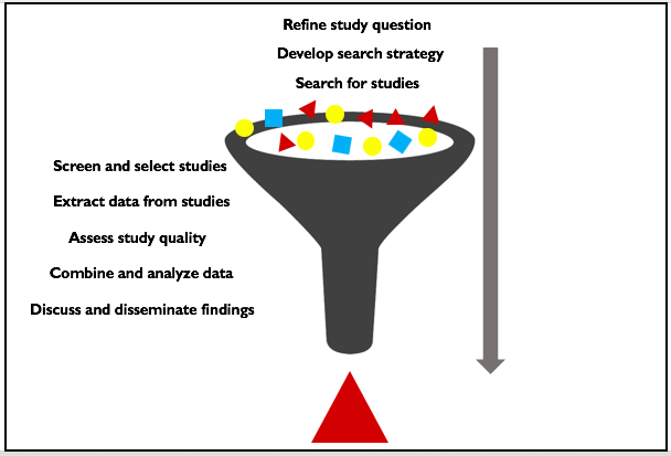
The steps in a systematic review
A systematic review begins with a well-defined research question. The figure below indicates the step-by-step process used to search for studies, identify studies for inclusion, carry out analyses and report findings.
The role of an information expert
Given the need for comprehensive, reproducible searches and intensive information management, trained librarians and information professionals are a critical component to performing a high quality systematic review.
Information specialists and librarians can assist in the following ways:
- Refining the research topic to an answerable research question appropriate for a systematic review.
- Developing search strategies, including identifying sources to search, harvesting search terms, and designing Boolean search across various databases.
- Gathering and deduplicating bibliographic records resulting from comprehensive database searches.
Automating systematic reviews
Systematic reviews are intensive, time-consuming projects often involving multi-person teams over many months or even 1-2 years or more. Thus, much is underway to identify ways in which parts of the process can be sped up, facilitated or automated.
The R package litsearchr provides a method to facilitate the harvesting of search terms to develop comprehensive search strategies, and to automatically create Boolean searches from lists of keywords, including incorporation of truncation and phrases.
Think-Pair-Share: Reproducibility and search strategies
Think about the process of developing a search strategy for a systematic review. What aspects of this process are reproducible? What aspects are more difficult to reproduce? How do you think a tool like R and litsearchr can help to increase the reproducibility of this process? Share your thoughts with your breakout room group, and then share with the rest of the group by adding a comment to the Etherpad.
Key Points
Systematic reviews differ from traditional literature reviews in a number of significant ways
Systematic review methods strive to reduce bias and increase reproducibility and transparency
Automation and coding software like R can be used to facilitate parts of the systematic review process
Introduction to RStudio
Overview
Teaching: 30 min
Exercises: 15 minQuestions
How to navigate RStudio?
How to run r code?
Objectives
Successfully navigate and run r code
What is R?
R is more of a programming language than a statistics program. You can use R to create, import, and scrape data from the web; clean and reshape it; visualize it; run statistical analysis and modeling operations on it; text and data mine it; and much more.
R is also free and open source, distributed under the terms of the GNU General Public License. This means it is free to download and use the software for any purpose, modify it, and share it. As a result, R users have created thousands of packages and software to enhance user experience and functionality.
When using R, you have a console window with a blinking cursor, and you type in a command according to the R syntax in order to make it do something. This can be intimidating for people who are used to Graphical User Interface (GUI) software such as Excel, where you use the mouse to point and click, and never or seldom have to type anything into the interface in order to get it to do something. While this can be seen as a drawback, it actually becomes a great advantage once you learn the R language, as you are not bound by the options presented to you in a GUI, but can craft flexible and creative commands.
What is RStudio?
RStudio is a user interface for working with R. You can use R without RStudio, but it’s much more limiting. RStudio makes it easier to import datasets, create and write scripts, and has an autocomplete activated for functions and variables you’ve already assigned. RStudio makes using R much more effective, and is also free and open source.
RStudio Console
After you install and open RStudio, you will see a window with four panes. You may need to open the top left “Source” pane by clicking on the maximize icon.
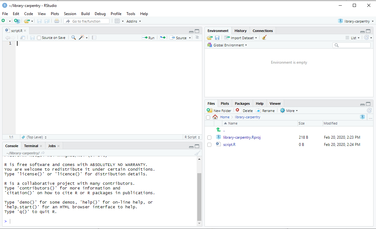
Console Pane (bottom left)
If you were just using the basic R interface, without RStudio, this is all you would see. You use this to type in a command and press enter to immediately evaluate it. It includes a > symbol and a blinking cursor prompting you to enter some code. You can type R code into the bottom line of the RStudio console pane and then click Enter to run it. The code you type is called a command, because it will command your computer to do something for you. The line you type it into is called the command line.
When you type a command at the prompt and hit Enter, your computer executes the command and shows you the results. Then RStudio displays a fresh prompt for your next command. For example, if you type 1 + 1 and hit Enter, RStudio will display:
## type in 1 plus 1
> 1+1
[1] 2
>
Code that you type directly in the console will not be saved, though it is available in the History Pane.
Script Pane (top left)
This is sort of like a text editor, or a place to write and save code. You then tell RStudio to run the line of code, or multiple lines of code, and you can see it appear in the console as it is running. Then save the script as a .R file for future use, or to share with others.
To execute code you use Ctrl+Enter (Cmd+Enter on a Mac). To create a new .R script file, use File > New File > R Script, and to open a script, use File > Open, or Recent Files to see files you’ve worked with recently. Save the R script by going to File > Save.
If you type an incomplete command and you execute it, R will display a + prompt, which means R is waiting for you to type the rest of your command. Either finish the command or hit Escape to start over:
## type in 6 subtracted from and leave it blank
> 6 -
+
+ 1
[1] 5
If you type a command that R doesn’t recognize, R will return an error message.
## type in 3 % 7
> 3 % 7
Error: unexpected input in 3 % 7
>
Once you understand the command line, you can easily do anything in R that you would do with a calculator. In its simplest form, R can be used as an interactive calculator.
## type in 5 plus 7
> 5 + 7
[1] 12

## type in 2 multiplied by 4
> 2 * 4
## 8

## type in 8 subtracted by 1
> 8 - 1
## 7

## type in 6 divided by (3 -1)
> 6 / (3 - 1)
## 3
Environment & History Pane (top right)
This pane includes two different but important functions.
The Environment will display the objects that you’ve read into what is called the “global environment.” When you read a file into R, or manually create an R object, it enters into the computer’s working memory. When we manipulate or run operations on that data, it isn’t actually written to a file until we tell it to. It is kept here in the environment.
The environment pane will also include any objects you have defined. For example, if you type y <- 5 into the console, you will now see y defined as a value in your environment.
You can list all objects in the environment by typing ls() in the console and pressing Enter on your keyboard. You can clear all objects in the environment by clicking the broom icon to the right of the words “Import Dataset.”. Clear individual objects by using the rm() function; for example: rm(y) will delete the y object from your environment. Practice typing in the following functions.
## to create object y type
y <- 5

## to list all objects in the  environment type
ls()

## to remove object y type
rm(y)
R treats the hashtag character, #, in a special way; R will not run anything that follows a hashtag on a line. This makes hashtags very useful for adding comments and annotations to your code. Humans will be able to read the comments, but your computer will pass over them. The hashtag is known as the commenting symbol in R.
Navigation pane (lower right)
This pane has multiple functions:
- Files: Navigate to files saved on your computer
- Plots: View plots (charts and graphs) you have created
- Packages: view add-on packages you have installed, or install new packages
- Help: Read help pages for R functions
- Viewer: View local web content
Challenge
Take a few minutes to practice executing commands and typing in the script pane with some basic arithmetic.
Solution
- To create object y. Answer: type
y <- 5- To multiply. Answer: type
2 * 4- To subtract. Answer: type
8 - 1- To divide. Answer: type
6 / (3 - 1)
Now that you feel more comfortable typing in commands let’s practice some more. Work through the following exercise:
Exercise
This exercise is to get you familiar with typing and executing commands in RStudio. Don’t worry about understanding the functions just yet. We’ll cover these in later episodes of this lesson.
- Create a new .R file called
my_first_script.R.- Type in
file.create("my_first_script.R")in the script pane.- Write each line of the following code separately in the script pane and identify where the results are found. To execute code you use Ctrl+Enter (Cmd+Enter on a Mac).
## to create a new .R file
file.create("my_first_script.R")
## type and run each line separately 2 + 2 sum(2, 2) sqrt(2) 2 + sqrt(4) y <- 5 y + y 2 * y print(y) View(y) str(y) plot(y) class(y) is.numeric(y) z <- c(5, 10, 15) y + z sum(y, z) plot(z) ls() rm(y) history()
Key Points
RStudio is a user interface for working with R.
The Script Pane is sort of like a text editor, or a place to write and save code.
To execute code you use Ctrl+Enter (Cmd+Enter on a Mac).
If you type an incomplete command and press Enter, R will display a
+prompt, which means R is waiting for you to type the rest of your command.If you type a command that R doesn’t recognize, R will return an error message.
The Environment Pane will display the objects that you’ve read into and objects you have defined.
The Navigation Pane has many functions: files, plots, packages, viewer, and help.
Create a Working Directory
Overview
Teaching: 20 min
Exercises: 20 minQuestions
How to create a working directory?
Objectives
Successfully set up a working directory in RStudio
Getting set up
You will need to create and set up your working directory in RStudio for this lesson. The working directory is very important, as it is the place where you will store, save, and retrieve your files. RStudio projects makes it easy to set up your working directory.
For this lesson we’ll create a new project.
-
Under the
Filemenu, click onNew project, chooseNew directory, thenNew project -
Enter a name for this new project
library-carpentry, and choose your desktop as the location. -
Click on
Create project
If for some reason your working directory is not set up correctly you can change it in the RStudio interface by navigating in the file browser where your working directory should be, and clicking on the blue gear icon “More”, and select “Set As Working Directory”.
If you haven’t already, download the workshop files, unzip or decompress the folder and place it into your new library-carpentry project directory by dragging and dropping file.
Make sure the files you downloaded from the zip folder are organized correctly before continuing on.
If you need to reorganize your files the instructions are below:
Create three folders on your computer desktop and name them
data,anderson_naive, andsearch_resultsAdd the following files you downloaded at the beginning of the lesson to the
datafolder.
- anderson_refs.csv
- anderson_refs.rda
- andersosn_studies.rda
- suggested_keywords_grouped
Add the three downloaded files from the anderson_naive zip folder to the
anderson_naivefolder.
- MEDLINE_1-500
- MEDLINE_501-603
- PsycINFO
Add the three downloaded savedrecs files to the
search_resultsfolder.
- savedrecs(1)
- savedrecs(2)
- savedrecs(3)
Add your three new folders,
data,anderson_naive, andsearch_resultsto thelibrary-carpentryfolder you just created.
Set your working directory
The working directory is the location on your computer R will use for reading and writing files. Use getwd() to print your current working directory to the console. Use setwd() to set your working directory.
# Determine which directory your R session is using as its current working directory using getwd().
getwd()
To set your new working directory go to:
- Under
Sessionat the top - Scroll down to
Set Working Directory - Select
Choose Directory - Choose the folder
lc_litsearchron your desktop
Organize your working directory
Using consistent filing naming and folder structure across your projects will help keep things organized. It will also make it easy to find things in the future since systematic reviews typically take months to complete. This can be especially helpful when you are working on multiple reviews or checking in with a review team months after running the initial search. In general, you can create directories or folders for scripts, data, and documents.
For this lesson, we will create the following in your working directory:
-
search_results_data/Use this folder to store your raw data or the original files you export from a bibliographic database. For the sake of transparency and provenance, you should always keep a copy of your raw data accessible and do as much of your data cleanup and preprocessing programmatically (i.e., with scripts, rather than manually) as possible. -
search_results_data_output/When you need to modify your raw data for your analyses, it might be useful to store the modified versions of the datasets generated by your scripts in a different folder. -
documents/This would be a place to keep outlines, drafts, and other text. -
scripts/This would be the location to keep your R scripts for different analyses or plotting.
You may want additional directories or subdirectories depending on your project needs, but these should form the backbone of your working directory for this lesson.
We can create these folders using the RStudio interface by clicking on the “New Folder” button in the file pane (bottom right), or directly from R by typing in the console.
# Use dir.create() to create directories in the current working directory called "search_results_data", "search_results_data_output", "documents", and "scripts".

dir.create("search_results_data")
dir.create("search_results_data_output")
dir.create("documents")
dir.create("scripts")
Exploring your working directory
Create a new object by assigning 8 to x using x <- 8.
x <- 8
You can list all the objects in your local workspace using ls(). See if the object x is listed.
ls()
Now, list all the files in your working directory using list.files() or dir().
dir()
As we go through this lesson, you should be examining the help page for each new function. Check out the help page for list.files with the command ?list.files.
?list.files
One of the most helpful parts of any R help file is the See Also section. Read that section for list.files.
Using the args() function on a function name is also a handy way to see what arguments a function can take. Use the args() function to determine the arguments to list.files().
args(list.files)

function (path = ".", pattern = NULL, all.files = FALSE,
    full.names = FALSE, recursive = FALSE, ignore.case = FALSE,
    include.dirs = FALSE, no.. = FALSE)
NULL
Create a file in your working directory called “mylesson.R” by using the file.create() function.
file.create("mylesson.R")
Typing in list.files() shows that the directory contains mylesson.R.
list.files()
You can check to see if “mylesson.R” exists in the working directory by using the file.exists() function.
file.exists("mylesson.R")
You can change the name of the file “mylesson.R” to “myscript.R” by using file.rename().
file.rename("mylesson.R", "myscript.R")
You can make a copy of “myscript.R” called “myscript2.R” by using file.copy().
file.copy("myscript.R", "myscript2.R")
Key Points
The working directory is very important, as it is the place where you will store, save, and retrieve your files.
Using consistent filing naming and folder structure across your projects will help keep things organized.
Download the file for this lesson if you haven’t done so already.
Importing Data into R
Overview
Teaching: 15 min
Exercises: 15 minQuestions
How to import data into R?
Objectives
Successfully import data into R
Importing data into R
In order to use your data in R, you must import it and turn it into an R object. There are many ways to get data into R.
- Manually: You can manually create it. To create a data.frame, use the
data.frame()and specify your variables. - Import it from a file Below is a very incomplete list
- Text: TXT (
readLines()function) - Tabular data: CSV, TSV (
read.table()function orreadrpackage) - Excel: XLSX (
xlsxpackage) - Google sheets: (
googlesheetspackage) - Statistics program: SPSS, SAS (
havenpackage) - Databases: MySQL (
RMySQLpackage) - Gather it from the web: You can connect to webpages, servers, or APIs directly from within R, or you can create a data scraped from HTML webpages using the
rvestpackage. - For example, connect to the Twitter API with the
twitteRpackage, or Altmetrics data withrAltmetric, or World Bank’s World Development Indicators withWDI.
Make sure the files you downloaded from the zip folder are organized correctly before continuing on.
If you need to reorganize your files the instructions are below:
Create three folders on your computer desktop and name them
data,anderson_naive, andsearch_resultsAdd the following files you downloaded at the beginning of the lesson to the
datafolder.
- anderson_refs.csv
- anderson_refs.rda
- andersosn_studies.rda
- suggested_keywords_grouped
Add the three downloaded files from the anderson_naive zip folder to the
anderson_naivefolder.
- MEDLINE_1-500
- MEDLINE_501-603
- PsycINFO
Add the three downloaded savedrecs files to the
search_resultsfolder.
- savedrecs(1)
- savedrecs(2)
- savedrecs(3)
Create a folder on your desktop called
lc_litsearchr. Add your three new folders,data,anderson_naive, andsearch_resultsto thelc_litsearchrfolder.If you need to download the files they can be found in Data
Opening a .csv file
To open a .csv file we will use the built in read.csv(...) function, which reads the data in as a data frame, and assigns the data frame to a variable using the <- so that it is stored in R’s memory.
## import the data and look at the first six rows
## use the tab key to get the file option
anderson_refs <- read.csv(file = "./data/anderson_refs.csv", header = TRUE, sep = ",")

head(anderson_refs)
## We can see what R thinks of the data in our dataset by using the class() function with $ operator.

# use the column name `year`
class(anderson_refs$year)

# use the column name `source`
class(anderson_refs$source)
The
headerArgumentThe default for
read.csv(...)is to set the header argument toTRUE. This means that the first row of values in the .csv is set as header information (column names). If your data set does not have a header, set the header argument toFALSE.
The
na.stringsArgumentWe often need to deal with missing data in our dataset. A useful argument for the read.csv() function is na.strings, which allows you to specify how you have represented missing values in the dataset you’re importing, and recode those values as NA, which is how R recognizes missing values. For example, if our anderson_refs dataset had missing values coded as lowercase ‘na’, we can recode these to uppercase ‘NA’ using the na.strings arguments as follows:
## To import data use the read.csv() function. To recode missing values to NA, use the `na.strings` argument

read.csv(anderson_refs, file = 'data/anderson_refs_clean.csv', na.strings = "na")
The
write.csvFunctionAfter altering a dataset by replacing columns or updating values you can save the new output with
write.csv(...).## To export the data use the write.csv() function. It requires a minimum of two arguments for the data to be saved and the name of the output file. ## For example, if we had edited the anderson_refs csv file we could use: write.csv(anderson_refs, file = "./data/anderson-refs-cleaned.csv")
The
row.namesArgumentThis argument for the write.csv function allows us to set the names of the rows in the output data file. R’s default for this argument is TRUE, and since it does not know what else to name the rows for the dataset, it resorts to using row numbers. To correct this, we can set row.names to FALSE:
## To export data use the write.csv() function. To avoid an additional column with row numbers, set `row.names` to FALSE

write.csv(anderson_refs, file = 'data/anderson_refs_clean.csv', row.names = FALSE)
Key Points
There are many ways to get data into R. You can import data from a .csv file using the read.csv(…) function.
Interacting with R
Overview
Teaching: 15 min
Exercises: 10 minQuestions
How to program in R?
Objectives
Successfully run multiple lines of R code
Interacting with R
R is primarily a scripting language, and written line-by-line. This can be quite useful; scripts can be assembled and built upon as you go into more substantial programs or compilations for analysis, but still editable at each line. There is no need to rerun the whole script in order to change a line of code. Many useful R code is written by the community through a variety of R packages available through CRAN (the Comprehensive R Archive Network), and other repositories. The ease with which packages can be developed, released, and shared has played a large role in R’s popularity. R packages can be thought of as libraries for other languages, as they contain related functions designed to work together. Packages are often created to streamline a common workflow.
The strength of R is in it’s interactive data analysis. A related strength, with packages like knitr and R Markdown, is in making the process and results easy to reproduce and share with others. Data in R are stored in variables and each variable is a container for data in a particular structure. There are four data structures most commonly used in R: vectors, matrices, data frames, and lists.
As we saw earlier in the lesson, you can use R like a calculator when you type expressions into the prompt, and press the Crtl + Enter keys (Windows & Linux) or Cmd+Return keys (Mac) to evaluate those expressions. Whenever you see the word Enter in the following steps of this lesson use the keys that work for your operating system in its place.
6 + 6
## [1] 12
You can use R to assign values, such as a numeric value like 4, and create objects. We will use the assignment operator to do this.This is the angle bracket (AKA the “less than”” symbol): <, which you’ll get by pressing Shift + comma and the hyphen - which is located next to the zero key. There is no space between them, and it is designed to look like a left pointing arrow <-.
# assign 4 to y by typing this in the console and pressing Enter
y <- 4
You have now created a symbol called y and assigned the numeric value 4 to it. When you assign something to a symbol, nothing happens in the console, but in the Environment pane in the upper right, you will notice a new object, y.
You can use R to evaluate expressions. Try typing y into the console, and press Enter on your keyboard, R will evaluate the expressions. In this case, R will print the elements that are assigned to y.
# evaluate y
y
## [1] 4
We can do this easily since y only has one element, but if you do this with a large dataset loaded into R, it will obliterate your console because it will print the entire dataset.
You can use R to type commands into your code by using the hash symbol #. Anything following the hash symbol will not be evaluated. Adding notes, comments, and directions along the way helps to explain your code to someone else as well as document your own steps like a manual you can refer back to. Commenting code, along with documenting how data is collected and explaining what each variable represents, is essential to reproducible research.
Vectors
The simplest and most common data structure in R is the vector. It contains elements of exactly one data type. Those elements within a vector are called components. Components can be numbers, logical values, characters, and dates to name a few. Most base functions in R work when given a vector as an argument. Everything you manipulate in R is called an object and vectors are the most basic type of object. In this episode we’ll take a closer look at logical and character vectors.
The c() function
The c() function is used for creating a vector. Read the help files for c() by calling help(c) or ?c to learn more.
## create a numeric vector num_vect that contains the values 0.5, 55, -10, and 6.
num_vect <- c(0.5, 55, -10, 6)
## create a variable called tf that gets the result of num_vect < 1, which is read as 'num_vect is less than 1'.
tf <- (num_vect < 1)
## Print the contents of tf.
tf
[1]  TRUE FALSE  TRUE FALSE

## tf is a vector of 4 logical values
The statement num_vect < 1 is a condition and tf tells us whether each corresponding element of our numeric vector num_vect satisfies this condition. The first element of num_vect is 0.5, which is less than 1 and therefore the statement 0.5 < 1 is TRUE. The second element of num_vect is 55, which is greater than 1, so the statement 55 <1 is FALSE. The same logic applies for the third and fourth elements.
Character vectors are also very common in R. Double quotes are used to distinguish character objects, as in the following example.
## Create a character vector that contains the following words: "My", "name", "is". Remember to enclose each word in its own set of double quotes, so that R knows they are character strings. Store the vector in a variable called my_char.

my_char <- c("My", "name", "is")

my_char
[1] "My"   "name" "is"
Right now, my_char is a character vector of length 3. Let’s say we want to join the elements of my_char together into one continuous character string (a character vector of length 1). We can do this using the paste() function.
## Type paste(my_char, collapse = " "). Make sure there's a space between the double quotes in the `collapse` argument.

paste(my_char, collapse= " ")
[1] "My name is"

## The `collapse` argument to the paste() function tells R that when we join together the elements of the my_char character vector, we would like to separate them with single spaces.
## To add your name to the end of my_char, use the c() function like this: c(my_char, "your_name_here"). Place your name in double quotes, "your_name_here". Try it and store the result in a new variable called my_name.

my_name <- c(my_char, "Amelia")

## Take a look at the contents of my_name.
my_name
[1] "My"     "name"   "is"     "Amelia"

## Now, use the paste() function once more to join the words in my_name together into a single character string.

paste(my_name, collapse = " ")
[1] "My name is Amelia"

## We used the paste() function to collapse the elements of a single character vector.
In the simplest case, we can join two character vectors that are each of length 1 (i.e. join two words). paste() can also be used to join the elements of multiple character vectors.
## Try paste("Hello", "world!", sep = " "), where the `sep` argument tells R that we want to separate the joined elements with a single space.

> paste("Hello", "world!", sep = " ")
[1] "Hello world!"
Functions
Functions are one of the fundamental building blocks of the R language. They are small pieces of reusable code that can be treated like any other R object. Functions are usually characterized by the name of the function followed by parentheses.
## The Sys.Date() function returns a string representing today's date. Type Sys.Date() below and see what happens.
Sys.Date()
Most functions in R return a value. Functions like Sys.Date() return a value based on your computer’s environment, while other functions manipulate input data in order to compute a return value.
The mean() function takes a vector of numbers as input, and returns the average of all of the numbers in the input vector. Inputs to functions are often called arguments. Providing arguments to a function is also sometimes called passing arguments to that function.
## Arguments you want to pass to a function go inside the functions parentheses. Try passing the argument c(2, 4, 5) to the mean() function.

> mean(c(2, 4, 5))
[1] 3.666667
We’ve used a couple of functions already in this lesson while you were getting familiar with the RStudio environment. Let’s revisit some of them more closely.
We can use names() to view the column head names in our csv file.
## to view the column head names in anderson_refs use the names() function
names(anderson_refs)
Since we’re dealing with categorical data in our csv file we can use the levels() function to view all the categories within a particular categorical column.
## to see all of the journals from the search results in anderson_refs use the levels() function
levels(anderson_refs$source)
However, if we try to use the levels() function on a non-categorical column like volume R will return a NULL
## try using levels() with a the volume number column
levels(anderson_refs$volume)

> levels(anderson_refs$volume)
NULL
We can use the sort() function to view all of the publication years sorted from oldest to most recent.
## to arrange publication years by asending order use the sort() function
sort(anderson_refs$year)
We can use the table() function to make a table from one of our categorical columns.
## to create a table counting how many times a journal appears in our search results
table(anderson_refs$source)
Learning R
-
swirlis a package you can install in R to learn about R and data science interactively. Just typeinstall.packages("swirl")into your R console, load the package by typinglibrary("swirl"), and then typeswirl(). Read more at http://swirlstats.com/. -
Try R is a browser-based interactive tutorial developed by Code School.
-
Anthony Damico’s twotorials are a series of 2 minute videos demonstrating several basic tasks in R.
-
Cookbook for R by Winston Change provides solutions to common tasks and problems in analyzing data
-
If you’re up for a challenge, try the free R Programming MOOC in Coursera by Roger Peng.
-
Books:
- R For Data Science by Garrett Grolemund & Hadley Wickham [free]
- An Introduction to Data Cleaning with R by Edwin de Jonge & Mark van der Loo [free]
- YaRrr! The Pirate’s Guide to R by Nathaniel D. Phillips [free]
- Springer’s Use R! series [not free] is mostly specialized, but it has some excellent introductions including Alain F. Zuur et al.’s A Beginner’s Guide to R and Phil Spector’s Data Manipulation in R
Key Points
R is primarily a scripting language, and written line-by-line.
There is no need to rerun the whole script in order to change a line of code.
The strength of R is in it’s interactive data analysis.
You can use R to assign values, such as a numeric value like 4, and create objects.
Dataframes, Matrices, and Lists
Overview
Teaching: 15 min
Exercises: 15 minQuestions
What is a dataframe in R?
How do you create a dataframe?
What are matrices in R?
Objectives
Successfully create a dataframe
Successfully explore a dataframe
Successfully use matrices in R
Data frames, Matrices, and Lists
Dataframes and matrices represent ‘rectangular’ data types, meaning that they are used to store tabular data, with rows and columns. The main difference is that matrices can only contain a single class of data, while data frames can consist of many different classes of data.
A data frame is the term in R for a spreadsheet style of data: a grid of rows and columns. The number of columns and rows is virtually unlimited, but each column must be a vector of the same length. A dataframe can comprise heterogeneous data: in other words, each column can be a different data type. However, because a column is a vector, it has to be a single data type.
Matrices behave as two-dimensional vectors. They are faster to access and index than data frames, but less flexible in that every value in a matrix must be of the same data type (integer, numeric, character, etc.). If one is changed, implicit conversion to the next data type that could contain all values is performed.
Lists are simply vectors of other objects. Lists are the R objects which contain elements of different types like − numbers, strings, vectors and another list inside it. This means that we may have lists of matrices, lists of dataframes, lists of lists, or a mixture of essentially any data type. This flexibility makes lists a popular structure. List is created using the list() function.
## Create a vector containing the numbers 1 through 20 using the `:` operator. Store the result in a variable called my_vector.
my_vector <- 1:20
## View the contents of the vector you just created.
my_vector
 [1]  1  2  3  4  5  6  7  8  9 10 11 12 13 14 15 16 17 18 19 20
## The dim() function tells us the 'dimensions' of an object.
dim(my_vector)
NULL

## Since my_vector is a vector, it doesn't have a
`dim` attribute (so it is just NULL),
## Find length of the vector using the length() function.
length(my_vector)
[1] 20
## If we give my_vector a `dim` attribute, the first number is the number of rows and the second is the number of columns.
## Therefore, we just gave my_vector 4 rows and 5 columns.
dim(my_vector) <- c(4, 5)
## Now we have turned the vector into a matrix. View the contents of my_vector now to see what it looks like.

my_vector
     [,1] [,2] [,3] [,4] [,5]
[1,]    1    5    9   13   17
[2,]    2    6   10   14   18
[3,]    3    7   11   15   19
[4,]    4    8   12   16   20
## We confirm it's actually a matrix by using the class() function.
class(my_vector)
[1] "matrix"
## We can store it in a new variable that helps us remember what it is.
my_matrix <- my_vector
A more direct method of creating the same matrix uses the matrix() function.
## Let's create a matrix containing the same numbers (1-20) and dimensions (4 rows, 5 columns) by calling the matrix() function.
## We will store the result in a variable called my_matrix2.

my_matrix2 <- matrix(1:20, nrow = 4, ncol = 5, byrow = FALSE)
Now, imagine that the numbers in our table represent some measurements from a library check out, where each row represents one library patron and each column represents one variable for how many items they’ve checked out a particular library item.
## We may want to label the rows, so that we know which numbers belong to which library patron.
## To do this add a column to the matrix, which contains the names of all four library patrons.

## First, we will create a character vector containing the names of our library patrons -- Erin, Kate, Kelly, and Matt.
## Remember that double quotes tell R that something is a character string. Store the result in a variable called patients.

library_patrons <- c("Erin", "Kate", "Kelly", "Matt")
## Use the cbind() function to 'combine columns'. Don't worry about storing the result in a new variable.
## Just call cbind() with two arguments -- the library patrons vector and my_matrix.
cbind(library_patrons, my_matrix)

    library_patrons
[1,] "Erin"   "1" "5" "9"  "13" "17"
[2,] "Kate"   "2" "6" "10" "14" "18"
[3,] "Kelly"  "3" "7" "11" "15" "19"
[4,] "Matt"   "4" "8" "12" "16" "20"
## Remember, matrices can only contain ONE class of data.
## When we tried to combine a character vector with a numeric matrix, R was forced to 'coerce' the numbers to characters, hence the double quotes.

## Instead we will create a data frame.
my_data <- data.frame(library_patrons, my_matrix)
## View the contents of my_data to see what we've come up with.
my_data

  library_patrons X1 X2 X3 X4 X5
1     Erin  1  5  9 13 17
2     Kate  2  6 10 14 18
3    Kelly  3  7 11 15 19
4     Matt  4  8 12 16 20

## the data.frame() function allowed us to store our character vector of names right alongside our matrix of numbers.
The data.frame() function takes any number of arguments and returns a single object of class data.frame that is composed of the original objects.
## confirm this by calling the class() function on our newly created data frame.
class(my_data)
[1] "data.frame"
We can also assign names to the columns of our data frame so that we know what type of library material each column represents.
## First, we'll create a character vector called cnames that contains the  following values (in order) -- "name", "book", "dvd", "laptop", "article", "reference".

cnames <- c("name", "book", "dvd", "laptop", "article", "reference")
## Use the colnames() function to set the `colnames` attribute for our data frame.
colnames(my_data) <- cnames
## Print the contents of my_data to see if all looks right.

my_data

    name  book  dvd laptop article reference
1    Erin   1    5     9     13       17
2    Kate   2    6    10     14       18
3   Kelly   3    7    11     15       19
4    Matt   4    8    12     16       20
Key Points
A data frame is the term in R for a spreadsheet style of data: a grid of rows and columns.
Lists are the R objects which contain elements of different types like − numbers, strings, vectors and another list inside it.
Matrices behave as two-dimensional vectors
Introduction to litsearchr
Overview
Teaching: 15 min
Exercises: 0 minQuestions
What is litsearchr?
What can it do?
Objectives
Provide context for litsearchr within the synthesis workflow
Explain what litsearchr can do
Explain how the litsearchr can help with systematic reviews
What is litsearchr and what does it do?
litsearchr is one part of the metaverse, a suite of integrated R packages that facilitate partial automation and reproducible evidence synthesis workflows in R.
Identify keywords
If you have ever had to iteratively test a search strategy for many hours, manually scanning articles for new keywords until you have identified all of the search terms needed to return a set of benchmark articles, you know how easy it can be to accidentally omit search terms. Even with iteratively testing a search strategy, keywords not included in the benchmark articles used to estimate the comprehensiveness of a search strategy can accidentally be omitted, which can limit the comprehensiveness of a systematic review. To quickly identify a suite of keywords that could be used as search terms for a systematic review and return potentially omitted terms, researchers and information specialists can supplement lists of terms identifed through conventional methods with terms identified by partially automated methods, which can reduce the time needed to deveop a search strategy while also increasing recall.
litsearchr is an R package that helps identify search terms to build more comprehensive search strategies and save time in selecting keywords. It does this by pulling out the most relevant keywords from articles on the research topic of interest and suggesting them as potential search terms. We will get more into the methods of how it does this and apply the methods in Search term selection with litsearchr.
Write and translate searches
Once users have identified search terms, either conventionally and/or with the partially automated approach, litsearchr automaticaly writes Boolean search strings and can translate searches into up to 53 languages by calling the Google Translate API. When writing searches, litsearchr can also lemmatize/truncate terms and remove redundant terms (e.g. “fragmented agricultural landscape” and “fragmented agriculture” can both be reduced to “fragmented agric*”).
Test search strategies
Finally, litsearchr can help automate the process of testing search strategies, reducing the amount of time it takes to check if the target articles are returned when estimating comprehensiveness and making the process repeatable because everything is documented in code.
Installing litsearchr
Because litsearchr is not on the CRAN repository yet, we need to install it with a slightly different approach than we used for other packages. We will use the remotes package to install it from GitHub and specify that the branch of the repository we want to install is main.
library(remotes)
install_github("elizagrames/litsearchr", ref="main")
Check-in with helpers
Key Points
litsearchr helps identify search terms and write Boolean searches for systematic reviews.
Developing a naive search and importing search results
Overview
Teaching: 30 min
Exercises: 20 minQuestions
What is the purpose of a naive search?
Objectives
Explain the characteristics of a good naive search and practice identifying components.
Work through the process of importing and deduplicating bibliographic data.
What is a naive search and how is it used?
To identify potential search terms, litsearchr extracts keywords from the results of a naive search. The goal of a naive search is to return a set of highly relevant articles to a topic, even if they may not meet all the criteria, because they will contain the best terms. A naive search should have high precision, as opposed to high recall, because if too many irrelevant articles are retrieved litsearchr will select vague keywords.
The reason for this is that litsearchr selects keywords based on how often they co-occur in the same article as other keywords; terms that co-occur frequently with other terms are classified as more important to the research topic since they are well-connected. If there are too many irrelevant articles in the naive search results, the terms that co-occur frequently across all the articles will be generic terms like “linear models” or “positive effect”, which clearly are not good keywords.
Coming up with a naive search is very similar to developing a search strategy with conventional methods, except without reading papers to identify terms. First, you want to identify the components of PICO (population, intervention, comparator, and outcome) for the review topic, or one of its variants, like TOPICS+M (Johnson & Hennessy 2019). Once these components or concept categories have been identified, come up with a set of the most precise terms you can think of that fit in the concept categories.
For example, if the population of interest is college students, you might come up with the terms “college student”, “undergraduates”, “post-secondary student”, “university student”, etc. You would not want to incude just “student” on its own since that could encompass earlier education stages or non-traditional education, and could result in many mis-hits for “Student’s t-test” which are not at all relevant.
Exercise: Develop a naive search
Working either alone or in small groups of 2-3, take 10 minutes to develop a naive search for this paper: “Impact of alcohol advertising and media exposure on adolescent alcohol use: a systematic review of longitudinal studies”. We will be using this systematic review by Anderson et al. (2009) throughout the lesson because it is open access and is of general public interest, but you can easily adapt the steps and code for your own research later.
Start by identifying the PICO (or one of its variants, such as PICOTS or PECO) components of the question and then generate all of the most precise synonyms. For example, you might opt for PECO and will identify the population as adolescents, exposure as alcohol advertising, and the outcome as alcohol use, but not include a comparator in the search terms.
Data used in this lesson
Normally once you have developed a naive search string, you would run the search in 2-3 databases appropriate for the topic and download the results in .ris or .bib format. You should make a note of which databases you searched, how many hits you got in each database, and any constraints you placed on the search for reproducibility.
The bibliographic data used in this lesson came from a search in MEDLINE (1990-2008) on Web of Science and PsycINFO (1990-2008) on EBSCO. We searched the title, abstract, keywords, and MESH fields using the naive search string below. We retrieved 603 results in MEDLINE and 71 in PsycINFO.
((teens OR teen OR teenager OR adolescent OR youth OR “high school”) AND (advertis* OR marketing OR television OR magazine OR “TV”) AND (alcohol OR liquor OR drinking OR wine OR beer))
Importing search results
Before we can work with bibliographic data in R, we first need to import it. To do this, litsearchr relies on its sister package synthesisr, which contains functions for manipulating bibliographic data and generic functions for working with text data. Import and deduplication can be done directly from litsearchr, or learners can try out the underlying functions directly in synthesisr for more flexibility.
First, we need to load litsearchr to use the functions in it. We do this with the library function, which loads all the functions and data in the litsearchr package.
library(litsearchr)
Now that we have loaded the library, we can use all the functions in litsearchr. The first function we will use is import_results, which as you might guess, imports bibliographic search results. Most functions in litsearchr have sensible names (but not all of them!) and you can view the help files for them using ?, such as ?import_results to determine what information needs to be passed to the function for it to work properly.
?import_results
There is no output from running this code, however, the Help panel will open up with information about import_results, including which arguments it takes. We have results saved in a directory (i.e. a folder), so we want to use the directory option rather than the file option, which would be for a single bibliographic file. Because the default option for verbose is TRUE, we do not need to specify it in order to have the function print status updates. Status updates are useful for importing results when you have a lot of results and want to make sure the function is working, or for diagnosing errors if the function fails to import a file and you want to know which one.
naive_import <- import_results(directory="./data/anderson_naive/")
## Reading file ./data/anderson_naive//MEDLINE_1-500.txt ... done
## Reading file ./data/anderson_naive//MEDLINE_501-603.txt ... done
## Reading file ./data/anderson_naive//PsycINFO.bib ... done
We can now check if all our search results were imported successfully. There were no errors in output, but we should also check that the correct number of results were imported. There should be 674 rows in the data frame because we had 603 search results in MEDLINE and 71 in PsycINFO. We can use nrow to print the number of rows in the data frame of imported search results to confirm this.
nrow(naive_import)
## [1] 674
Check-in with helpers
For virtual lessons: head to breakout rooms to check in with helpers.
Deduplicating search results
Some articles may be indexed in multiple databases. We need to remove duplicate articles because otherwise the terms found in those articles will be overrepresented in the dataset.
There are a lot of options for how to detect and remove duplicates. For example, you could remove articles that have the exact same title, or that have the same DOI, or that have abstracts which are highly similar to each other and may just differ by extra information that a database appends to the abstract field (e.g. starting with ABSTRACT: ). There are even more options for customizing deduplication if using the synthesisr package directly, but we will stick with a fairly simple deduplication because if a few duplicate articles are missed, it will not affect the keyword extraction too much.
Here, we will remove any titles that are identical. First, we need to check which fields exist in our dataset and what the name is for titles in our dataset.
colnames(naive_import)
##  [1] "publication_type" "status"           "author"           "researcher_id"    "year"             "date_published"
##  [7] "title"            "source"           "volume"           "issue"            "n_pages"          "abstract"
## [13] "version"          "doi"              "issn"             "nlm_id"           "accession_number" "accession_zr"
## [19] "published_elec"   "ZZ"               "orcid_id"         "title_foreign"    "author_group"     "A2"
## [25] "AU"               "type"             "journal"          "keywords"         "number"           "pages"
## [31] "url"              "school"           "booktitle"        "isbn"             "publisher"        "series"
## [37] "filename"
litsearchr will automatically ignore case and punctuation, so “TITLE:””, “title–””, and “Title”” are considered duplicates.
naive_results <- remove_duplicates(naive_import, field = "title", method = "exact")
Exercise: Counting unique records
Check how many unique records were retained with
nrow. Since there were only two databases, how many records can we conclude were unique to PsycINFO and not in the MEDLINE output?
Key Points
A good naive search provides a good basis for identifying potential search terms on a topic.
Search results should be deduplicated to avoid terms used in some papers being overrepresented.
Identifying potential keywords with litsearchr
Overview
Teaching: 30 min
Exercises: 15 minQuestions
How does litsearchr identify potential keywords?
Objectives
Explain how to extract potential terms using different methods.
Extracting potential keywords from naive search results
Now that we have our deduplicated results, we can extract a list of potential keywords from them. This is not the list of keywords you will want to consider including in your search (we will get to that in a bit), and is simply all of the terms that the keyword extraction algorithm identifies as being a possible keyword.
We can identify potential keywords with the extract_terms function. To use extract_terms, we have to give it the text from which to extract terms. Using the titles, abstracts, and author- or database-tagged keywords makes the most sense, so we will paste those together. To subset these columns from our data frame, we can use $ to extract named elements, which in our case are columns.
my_text <- paste(naive_results$title,
                 naive_results$abstract,
                 naive_results$keywords)
The method we will use to extract terms is called “fakerake” since it is an adaptation of the Rapid Automatic Keyword Extraction algorithm.
When working with your own data, you will want to tweak the options in extract_terms depending on how many articles are returned by your naive search and how specific you want the search term suggestions to be. If you have a lot of naive search results, you may want to increase min_freq to higher numbers; here, we are only requiring a term to appear twice anywhere in the text in order to be identified as a keyword. This removes many spurious keywords and unhelpful terms like specific locations where a study took place.
The next two arguments, ngrams and min_n, refer to whether or not litsearchr should only retrieve phrases of a certain length. There are very few situations where you will not want ngrams to equal TRUE; this is the tested method for litsearchr and what it is designed to do. Similarly, we recommend min_n = 2 because then all phrases with at least two words are suggested as keywords.
Lastly, the language argument is used to determine what stopwords (terms like “the”, “should”, “are”, etc.) will not be allowed as keywords.
raked_keywords <- extract_terms(
  text = my_text,
  method = "fakerake",
  min_freq = 2,
  ngrams = TRUE,
  min_n = 2,
  language = "English"
)
## Loading required namespace: stopwords
Check-in with helpers
For virtual lessons: head to breakout rooms to check in with helpers.
Inspecting identified keywords
We can view some of the keywords using head and specifying how many terms we want to view.
head(raked_keywords, 20)
##  [1] "abstract truncated"         "abuse education"            "abuse prevention"
##  [4] "abuse prevention programs"  "abuse treatment"            "academic performance"
##  [7] "active participation"       "active students"            "activities designed"
## [10] "activity habits"            "activity level"             "activity levels"
## [13] "activity patterns"          "actual alcohol"             "actual alcohol consumption"
## [16] "addictive behaviors"        "addictive substances"       "additional research"
## [19] "adequately studied"         "administered questionnaire"
Some of these are clearly not relevant (e.g. “additional research”), but terms like this will be removed in subsequent filtering steps. If we want to inspect keywords that contain certain terms, we can use grep to subset these terms and view them. This can be useful if you want to reassure yourself that good keywords were retrieved in the naive search.
Here, we are checking to see if terms related to alcohol were retrieved and make sense for this topic.
alcohol <- raked_keywords[grep("alcohol", raked_keywords)]
head(alcohol, 20)
##  [1] "actual alcohol"                 "actual alcohol consumption"     "adolescent alcohol"
##  [4] "adolescent alcohol consumption" "adolescent alcohol initiation"  "affect alcohol"
##  [7] "aggregate alcohol"              "alcohol abuse"                  "alcohol abuse education"
## [10] "alcohol abuse prevention"       "alcohol abusers"                "alcohol addiction"
## [13] "alcohol advertisement"          "alcohol advertisement exposure" "alcohol advertisements"
## [16] "alcohol advertisers"            "alcohol advertising"            "alcohol advertising effects"
## [19] "alcohol advertising exposure"   "alcohol advertising targeted"
Exercise: Subsetting keywords
Using what you have just learned, write R code that subsets out terms that contain “advertis”, similar to searching for advertis* to capture advertisement, advertising, advertiser, etc.
How many terms contain “advertis”? Hint:
lengthwill be useful.
Key Points
litsearchr helps identify potential search terms related to the topic of a systematic review.
Search term selection with litsearchr
Overview
Teaching: 30 min
Exercises: 20 minQuestions
How does litsearchr select important keywords?
Objectives
Explain the method litsearchr uses to identify important terms and work through this process.
How litsearchr identifies useful keywords
Because not all the keywords are relevant (and you probaby do not want to run a search with several thousand terms!), the next step is to determine which keywords are important to the topic of the systematic review and manually review those suggestions.
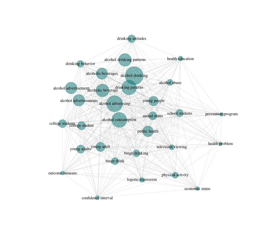
To do this, litsearchr puts all of the terms into a keyword co-occurrence network. What this means is that if two terms both appear in the title/abstract/keywords of an article, they get marked as co-occurring. Terms that co-occur with other terms frequently are considered to be important to the topic because they are well-connected, especially if they are connected to other terms that are also well-connected. Building the keyword co-occurrence network lets litsearchr automatically identify which terms are probably important and suggest them as potential keywords.
Assessing how important terms are
First, we will create a document-feature matrix. What litsearchr will do is take the list of potential keywords and determine which articles they appear in. We once again use our my_text object we created earlier by pasting together titles, abstracts, and keywords. These are the elements in which we want to look for occurrences of our features, which are the raked_keywords. This code creates a large simple triplet matrix, so it can take a little while to run.
naive_dfm <- create_dfm(
    elements = my_text,
    features = raked_keywords
  )
Now that we have a document-feature matrix, we can convert it to a network graph which makes it easy to to visualize relationships between terms and to assess their importance. We have the option to restrict how many studies a term must appear in to be included by using min_studies or how many times in total it appears with min_occ, however here we have left it the same as when we identified possible terms (2).
naive_graph <- create_network(
    search_dfm = as.matrix(naive_dfm),
    min_studies = 2,
    min_occ = 2
  )
Check-in with helpers
For virtual lessons: head to breakout rooms to check in with helpers.
Now that we have our network, we need to figure out which terms are the most important. One of the interesting things about keyword co-occurrence networks (and networks in general) is that their importance metrics follow a power law, where there are many terms with low importance and a few terms that are very important. To see what this looks like, we can extract the node strength from the network using the igraph package, sort the terms in order or their strenghts, and plot the node strengths.
# load the igraph library
library(igraph)

## Attaching package: ‘igraph’

## The following objects are masked from ‘package:stats’:

##    decompose, spectrum

## The following object is masked from ‘package:base’:

##    union
Next, we want to get the node strength for the graph and sort the strengths in decreasing order, so that the most important terms are at the top.
strengths <- sort(strength(naive_graph), decreasing=TRUE)

# then we can see the most important terms

head(strengths, 10)

##      alcohol consumption       alcohol advertising
##                     1556                      1106
##            public health          alcohol drinking
##                     1046                      1026
##        physical activity              young people
##                      993                       896
##          school students         drinking patterns
##                      839                       820
##            united states alcohol drinking patterns
##                      722                       660

# most of them look pretty relevant to the topic, which is good
To see what we mean by the network node strengths following a power law, let’s plot our sorted vector of strengths. We will use type="l" to plot a line, and las=1 to make our y-axis labels parallel with our x-axis so they are easy to read.
plot(strengths, type="l", las=1)
Check-in with helpers
For virtual lessons: head to breakout rooms to check in with helpers.
Selecting important terms
We can use this power law relationship as a way to identify important terms. We want all the terms above some cutoff in importance, and do not want to consider the terms in the tail of the distribution.
To find a cutoff in node importance, we can use the aptly-named find_cutoff function. With method cumulative, we can tell the function to return a cutoff that gives us the minimum number of terms that gives us 30% of the total importance in the network.
cutoff <- find_cutoff(
    naive_graph,
    method = "cumulative",
    percent = .30,
    imp_method = "strength"
  )

print(cutoff)
## [1] 162
Exercise: Changing cutoff stringency
In some cases, we may want to be more or less flexible with where the cutoff is placed for term importance. Using the code from the lesson as a template, find a new cutoff that returns 80% of the strength of the network.
Next, we want to reduce our graph (reduce_graph) to only terms that have a node strength above our cutoff value. We can then get the keywords (get_keywords) that are still included in the network, which will give us a vector of important keywords to manually consider whether or not they should be included in the search terms.
reduced_graph <- reduce_graph(naive_graph, cutoff_strength = cutoff)

search_terms <- get_keywords(reduced_graph)
Challenge: Counting search terms
How many terms has litsearchr suggested we review manually? Hint:
lengthwill be useful.
Bonus Challenge
How many more search terms are retrieved when using a threshold of 50% instead of 30% of the network strength?
Hint: you will need to find cutoff values for both 50% and 30%, create two new reduced graphs with the different cutoff strengths, and check the
lengthof the resulting search terms for each graph.
Key Points
litsearchr helps identify important search terms related to the topic of a systematic review.
Group search terms to concept categories
Overview
Teaching: 10 min
Exercises: 15 minQuestions
Can you add in more search terms that were not identified by litsearchr?
Objectives
Practice grouping search terms into concept categories and reading data.
Practice adding more keywords into the list of search terms.
Grouping keywords into concept categories
The output from the previous episode is a long list of suggested keywords, not all of which will be relevant. These terms need to be manually reviewed to remove irrelevant terms and to classify keywords into useful categories. Some keywords may fit into multiple components of PICO, in which case they can be grouped into both. Research teams should decide whether they want to decide on search terms in duplicate or singly.
To group keywords into categories, we recommend exporting the suggested list of keywords to a .csv file, manually tagging each keyword for either one of your PICO categories or as irrelevant, then reading the data back in. In this section, we will export a .csv file, enter data outside of R, read that data from a .csv file, and merge groups together.
Exercise: Grouping terms
First, use
write.csvto save the search_terms to a file on your computer.write.csv(search_terms, file="./suggested_keywords.csv")Next, open the exported .csv file in whatever software you use to work with spreadsheets (e.g. LibreOffice or Microsoft Excel). Add a column to the spreadsheet called ‘group’ and rename the column of terms ‘term’.
Take 3-5 minutes to go through as many terms in the list as you have time for and decide whether they match to the population (adolescents), exposure (alcohol advertising), outcome (alcohol use), or none of the groups. In the ‘group’ column of the spreadsheet, indicate the group(s) that a term belongs to; for example, “teen binge drinking” would be marked as “population, outcome” in the ‘group’ column because it matches two of the concept categories. For terms that are not relevant, you can mark the group as “x” or “not relevant” or another term that makes sense to you.
You should not expect to finish reviewing terms in that amount of time, but can practice classifying them. We will use a pre-filled out .csv for subsequent practice.
Reading grouped terms into R
We need to read the spreadsheet of grouped terms back into R so that litsearchr can use the categories to write a Boolean search. To do this, we will use read.csv to import our spreadsheet and then use head to confirm that the data we read in is what we expected based on the exercise. It will not be identical to the results from the exercise because we are using a pre-filled out .csv so that everyone has the same set of terms and can follow along.
grouped_terms <- read.csv("./data/suggested_keywords_grouped.csv")

head(grouped_terms)
Once terms have been manually grouped and read into a data frame in R, the terms associated with each concept group can be extracted to a character vector. Because all groups and terms will be different depending on the topic of a review, this stage is not automatically done by litsearchr and requires some custom coding to pull out the different groups.
We can use grep to determine which terms belong to each group; grep is a way to detect strings (i.e. words). The output of grep is a vector of numbers that indicate which elements from grouped_terms$group contain the term ‘population’ which we can use to subset them out. We can combine this with square brackets [] to subset the ‘term’ column of grouped_terms and extract just the ones that contain the pattern ‘population’.
grep(pattern="population", grouped_terms$group)

population <- grouped_terms$term[grep(pattern="population", grouped_terms$group)]
Exercise: Subsetting terms
Using what you just learned to subset the population terms, repeat this process for the outcome and exposure groups and save them to character vectors named
outcomeandexposure.
exposure <- grouped_terms$term[grep("exposure", grouped_terms$group)]outcome <- grouped_terms$term[grep("outcome", grouped_terms$group)]
Adding new terms to a search
Because litsearchr defaults to suggesting phrases with at least two words and may not pick up on highly specialized terms or jargon that appears infrequently in the literature, information specialists and researchers may want to add their own terms to the list of suggested keywords. This can easily be done with the append function.
For example, we may want to add back the terms from our naive search:
((teens OR teen OR teenager OR adolescent OR youth OR “high school”) AND (advertis* OR marketing OR television OR magazine OR “TV”) AND (alcohol OR liquor OR drinking OR wine OR beer))
To do this, we can use append to add more terms to the end of our character vector. If you do not know if a term was already in the list, add it anyways and use unique to keep only unique terms.
population <- append(population, c("teenager", "teen", "teens",
                                  "adolescent", "adolescents",
                                  "youth", "high school"))

exposure <- append(exposure, c("marketing", "television", "TV", "magazine"))

outcome <- append(outcome, c("alcohol", "liquor", "drinking", "wine", "beer"))
Check-in with helpers
For virtual lessons: head to breakout rooms to check in with helpers.
Key Points
litsearchr assumes keywords are grouped into distinct concept categories.
Write a Boolean search string with litsearchr
Overview
Teaching: 15 min
Exercises: 5 minQuestions
How does litsearchr write a Boolean search from the list of terms?
What are the different options for writing search strings?
Objectives
Explain the different options for writing Boolean search strings with litsearchr.
Options for writing a Boolean search with litsearchr
Now that all terms are selected and grouped, litsearchr can take a list of terms and turn them into a full Boolean search. Because each bibliographic database has slightly different assumptions about how search strings should be formatted, litsearchr has options for formatting, lemmatization/stemming, etc. We will review how to use all the different options and what they mean in terms of the logic of the final search in human terms. We encourage you to play with different combinations to get a sense of how the options interact with each other.
exactphrase
Should search terms be wrapped in quotes to retrieve the exact phrase? Although this is not universally the proper logic for bibliographic databases, it works on many common platforms, though note that if you are using Scopus or other platforms with irregular punctuation logic, you may need to replace “quotes” with {brackets} depending on the platform search guidance.
stemming
Should search terms be lemmatized (i.e. reduced to root word stems) and truncated with a wildcard marker? For example, “outdoor recreation” could be converted to “outdoor* recreat*” to also capture terms like “outdoors recreation” or “outdoor recreational”. There may be cases where researchers do not want this feature applied to subsets of words (e.g. “rat” and “rats” are not easily replaced by “rat*”), so it can be disabled (though by default, litsearchr only allows stems of 4 letters or longer). If only some terms should be stemmed and others (e.g. ratio*) should not be, there is no easy solution in litsearchr. We recommend using the stemming option in these cases, then manually cleaning up the final search for cases where stemming is not appropriate.
closure
By default, litsearchr removes redundant search terms to reduce the total length of a search string and to make it more efficient. For example, if search terms include “woodpecker”, “woodpecker abundance”, and “black-backed woodpecker”, only the term “woodpecker” needs to be searched because it is contained within the other two terms, so they are redundant and can be eliminated from the search. There may be cases where information specialists and researchers do not want redundant terms removed (e.g. when including the singular and plural form of a term is important for database search rules). To accommodate these cases, users can specify how they want terms to be detected as redundant based on assumptions of closure.
- left – If one term is the beginning of another term, the second term is redundant.
- right – If one term is the end of another term, the second term is redundant.
- full – Terms are only redundant if identical (after stemming, if this is an option).
- none – If a term appears anywhere inside another term, the second term is redundant.
Exercise: Understanding closure rules
To understand the closure rules, play around with some mock search terms by changing the closure, stemming, and exactphrase options and seeing how the outcput changes.
terms <- c("advertise", "advertising", "alcohol advertising", "advertisement")write_search(list(terms), closure="left", languages="English", stemming=TRUE, exactphrase=TRUE)
Writing a Boolean search
To actually write a Boolean search for our example systematic review, we should give litsearchr our full term list. We can then either copy the output to a database search, or change writesearch to TRUE and litsearchr will write the search to a plain text file.
full_search <- write_search(list(population, exposure, outcome),
                            closure = "none",
                            languages = "English",
                            stemming = TRUE,
                            exactphrase = TRUE,
                            writesearch = FALSE
                            )
print(full_search)
Check-in with helpers
For virtual lessons: head to breakout rooms to check in with helpers.
Key Points
Given a list of terms grouped by concept, litsearchr can write full Boolean search string from them.
Testing search strategy performance with litsearchr
Overview
Teaching: 20 min
Exercises: 20 minQuestions
How should benchmark articles be chosen and used?
How do you add missing search terms to retrieve benchmark articles?
Objectives
Explain how to check search string recall with litsearchr.
Practice identifying missing search terms with litsearchr.
Selecting benchmark articles
To estimate if a search string is comprehensive, we need a set of benchmark articles to test it against. Normally, these will come from previous reviews on similar topics or from a list suggested by subject experts. For this exercise, we will use the list of articles included in the original systematic review that we are using as an example. Although the original review included 16 articles, here, we only have 15 articles because one was in press at the time of the original article, so we know it will not be retrieved by our replicated searches as we set the years of articles to return to be from 1990-2008.
Not all of our benchmark articles will be indexed in the databases we are testing our search strategy in. To test our string, we really want to know if our search string can retrieve an article only if it is included in the database. The easiest way to check this is to search for the titles of the articles we want to retrieve in the databases we are using. To check this, we can use write_title_search, which is really just a special case of writing a Boolean search that does not allow stemming and retains all terms in the title.
load("./data/anderson_studies.rda")
benchmark <- anderson_studies$title

write_title_search(benchmark)
Check-in with helpers
For virtual lessons: head to breakout rooms to check in with helpers.
We can then copy the title search and see if the articles are indexed by searching the databases we are using. When you only have a handful of benchmark articles like in this case, it is fairly easy to manually check if they were retrieved. But what if you had a list of dozens, or even a hundred, benchmark articles and wanted to check whether they are retrieved across databases? That’s where partially automated search testing can be especially useful. The other benefit of testing search strategies in R is that the results are then reproducible and you can easily document what modifications were needed to retrieve all the benchmark articles and how those decisions were made.
Importing quasi-gold standard articles and search results
First, we need to read in the results of searching for titles in a database; this is our new gold standard. We also want to import the search results from the database(s) we are testing our search in. In this exercise, we will just test our search strategy in MEDLINE since all our benchmark articles are indexed in it.
# note that we use file as the argument here because we only have one file for the search result
gold_standard <- import_results(file="./data/search_testing/qgs.txt")

# but here, we use directory because we have saved several files to our search results folder
medline <- import_results(directory="./data/search_testing/search_results/")
Check-in with helpers
For virtual lessons: head to breakout rooms to check in with helpers.
Estimating search strategy comprehensiveness
We can now check if our gold standard articles are retrieved by the search with the check_recall function. It compares the similarity of our gold standard titles to the ones our search found and reports this information back. Articles with a similarity of 1 were almost certainly retrieved (though be careful if you ever have a benchmark article with an extremely generic title!), and anything below that should be manually checked to see if they are the same title.
recall <- check_recall(tolower(gold_standard$title), tolower(medline$title))
Exercise: Checking articles with low similarity
For our benchmark articles, we should manually review whether or not they were indeed retrieved if they have low similarity scores. To find articles below a certain similarity level, we will need to convert it to a number.
recall[,'Similarity'] <- as.numeric(recall[,'Similarity'])Now we can view articles with similarities below 1.
recall[which(recall[,'Similarity'] < 1),]Were all the benchmark articles retrieved?
Reproducibility of search testing
One of the nice things about testing search strategies in R is that your tests are reproducible. You can re-run the code with the same files and will get the same results. You can also save your workspace so you know exactly what the output was the last time you ran the code. This is especially helpful for testing search strategies, since you may tweak which terms you include in the search and want a record of which articles were retrieved.
To save the output of running your code, you can either write files like we have been doing (e.g. with write.csv) or you can save the R objects themselves. You can save everything in your Global Environment with save.image or you can save one or more individual objects with save. Here, we will save the full search we wrote, the results we got in MEDLINE, and the recall of our search string and name the file something sensible.
save(full_search, medline, recall, file="search_test_round1.rda")
If we then want to read those objects into R again, we can use load to read them into our workspace, or we could send the .rda file to a colleague who could also load the objects without having to run all the code or need the files you used to produce them.
Check-in with helpers
For virtual lessons: head to breakout rooms to check in with helpers.
Key Points
litsearchr can help test the recall (sensitivity) of search strategies.
Assessment
Overview
Teaching: 0 min
Exercises: 0 minQuestions
…
Objectives
…
Key Points
…