All in One View

Content from Introduction

Last updated on 2026-08-13 | Edit this page

Overview

Questions

What exactly is job efficiency in the computing world?
Why would I care about job efficiency and what are potential pitfalls?
How can I begin measuring the runtime performance of my programs?

Objectives

After completing this episode, participants should be able to:

Use time and date to measure program runtime.
Identify how implementation choices affect runtime, resource usage, and numerical results.
Explain how inefficient jobs affect resource consumption and energy usage.

Background

According to Oxford’s English Dictionaries, efficiency is “the ratio of the useful work performed by a machine […] to the total energy expended or heat taken in”.

In a High-Performance Computing (HPC) context, the useful work corresponds to the scientific computations performed by an application. Efficient execution therefore means making effective use of allocated computational resources such as CPU cores, memory, GPUs, storage systems, and interconnect bandwidth, while also minimizing runtime and energy consumption. Or, phrased more bluntly, we want to avoid running large HPC systems for nothing but hot air.

At first glance, a single inefficient job may seem to have little impact on overall power consumption of an HPC system, since such systems operate continuously anyway. A similar argument could be made about air travel: the airplane will take off regardless of whether one additional passenger boards the flight. However, individual behavior still contributes to overall efficiency. In air travel, passengers can improve fuel efficiency by traveling lightly and avoiding unnecessary baggage, thereby improving the airplane’s ratio $\frac{useful\;work}{total\;energy\;expended}$.

In HPC systems, users similarly influence overall system efficiency through the way they configure, execute, and optimize their workloads. Throughout this lesson, we will examine common inefficiencies in computational jobs while continuing to use the air-travel analogy to build intuition about resource utilization and performance optimization.

Before we can improve the efficiency of a computational workload, we first need a way to measure it. One of the simplest and most informative performance metrics is the runtime of a program. The time command provides a convenient way to obtain this measurement.

Measuring `sleep` with `time`

Let’s look at the sleep command.

BASH

sleep 2

This command pauses execution for a specified duration, here 2 seconds, before continuing with the next command. You can verify the pause duration using a stopwatch, here provided by the time command:

BASH

time sleep 2

which will produce output similar to

OUTPUT

real    0m2.002s
user    0m0.001s
sys     0m0.000s

The time command is often one of the first performance-analysis tools introduced in HPC. This command provides a breakdown of elapsed wall-clock time and CPU execution time consumed by your program. The time command reports three timing measurements: real, user, and sys.

Time	Meaning
real	Wall-clock time = total runtime as seen on a stopwatch
user	Time spent in user mode: application computations such as arithmetic operations, loops, and program logic
sys	Time spent in the operating system’s kernel mode (system calls): I/O = reading/writing files, memory management, and device communication

The sleep command performs almost no computations or I/O operations. As a result, the reported user and sys times remain close to zero.

Why does time sometimes produce different output?

You may notice that the output of time on your system looks different from the examples shown in this lesson. This is because time exists both as a shell keyword provided by your shell (such as Bash or zsh) and as a standalone executable, usually located at /usr/bin/time. When you run time <command>, the shell normally executes its own time keyword rather than the GNU executable. You can verify this with

BASH

$ which -a time
/usr/bin/time
$ type -a time
time is a shell keyword
time is /usr/bin/time

Notice that which only locates executables available through the user’s $PATH, whereas type also reports shell keywords and built-in commands. This makes type the more useful command for determining what will actually be executed.

If you specifically want to use the GNU implementation, invoke it by specifying its full path:

BASH

$ /usr/bin/time sleep 2
0.00user 0.00system 0:02.00elapsed 0%CPU (0avgtext+0avgdata 2176maxresident)k
0inputs+0outputs (0major+90minor)pagefaults 0swaps

The GNU implementation can also produce a more detailed report using the -v (“verbose”) option:

BASH

$ /usr/bin/time -v sleep 2
	Command being timed: "sleep 2"
	User time (seconds): 0.00
	System time (seconds): 0.00
	Percent of CPU this job got: 0%
	Elapsed (wall clock) time (h:mm:ss or m:ss): 0:02.00
	Average shared text size (kbytes): 0
	Average unshared data size (kbytes): 0
	Average stack size (kbytes): 0
	Average total size (kbytes): 0
	Maximum resident set size (kbytes): 1920
	Average resident set size (kbytes): 0
	Major (requiring I/O) page faults: 0
	Minor (reclaiming a frame) page faults: 105
	Voluntary context switches: 10
	Involuntary context switches: 1
	Swaps: 0
	File system inputs: 0
	File system outputs: 0
	Socket messages sent: 0
	Socket messages received: 0
	Signals delivered: 0
	Page size (bytes): 4096
	Exit status: 0

For comparison, the Bash shell keyword produces a much shorter summary:

BASH

$ time sleep 2

real    0m2.003s
user    0m0.001s
sys     0m0.003s

Different shells may format their output differently. For example, the time keyword in zsh reports:

BASH

$ time sleep 2
sleep 2  0.00s user 0.00s system 0% cpu 2.003 total

Although the formatting differs, all of these implementations report broadly the same runtime information. The main differences are the output format and, in the case of GNU /usr/bin/time, the amount of detail that is available.

For HPC users this distinction is occasionally important. Different HPC systems may use different login shells, shell versions, or software environments. As a result, the format of the output produced by time may differ between clusters even when the measured quantities are the same. This is particularly relevant when benchmarking or profiling workflows automatically parse the output of time, since different implementations may produce different field names or output formats.

Benchmarking and profiling

Runtime measurements are often collected automatically during performance studies.

Benchmarking measures how application performance changes under different execution conditions, such as varying the number of CPU cores, nodes, threads, problem sizes, or hardware configurations.
Profiling collects detailed information about how a program uses computational resources during execution. Typical profiling metrics include execution time, memory usage, communication overhead, I/O activity, and other performance-related measurements.

Because such workflows often process timing data automatically, differences in the output format produced by time may require special handling.

Benchmarking and profiling are commonly used to identify performance bottlenecks and evaluate optimization strategies for HPC applications.

Shell keywords and executables are documented differently. Shell keywords provide built-in help through help, for example

BASH

help time

whereas executables typically provide manual pages:

BASH

man time

Knowing which implementation you are using can help explain differences in reported runtime statistics across systems.

Callout

Different HPC systems may provide different default login shells or environment configurations. You can inspect available shells using:

BASH

$ cat /etc/shells

OUTPUT

/bin/sh
/bin/bash
/usr/bin/sh
/usr/bin/bash
/usr/bin/tmux
/bin/tmux
/bin/csh
/bin/tcsh
/usr/bin/csh
/usr/bin/tcsh
/bin/ksh
/bin/rksh
/usr/bin/ksh
/usr/bin/rksh

To determine your currently active shell, you can use:

BASH

$ echo "$SHELL"

OUTPUT

/bin/bash

Time for a `date`

The time command measures the runtime of an entire command. Sometimes, however, we want to measure only part of a workflow or record timestamps inside a shell script. In these situations, the date command provides a simple way to obtain precise timestamps.

As described in its manual page (man date), the date command prints or sets the system date and time. It can also be used as a lightweight source of high-resolution timestamps:

BASH

date +%s.%N

OUTPUT

1785152285.376560875

The exact output will vary each time the command is run.

The timestamp is expressed as the number of seconds elapsed since a fixed reference point.

Unlike time, which measures an entire command, recording timestamps with date allows us to measure selected parts of workflows or multiple commands within shell scripts.

Epoch time

To calculate elapsed time, timestamps must share a common reference point. Such a reference point is commonly called the epoch.

According to the date manual page, the default reference point used by date is 1970-01-01T00:00:00+00:00, commonly known as the Unix epoch.

BASH

date -u -d @0 --iso-8601=seconds

OUTPUT

1970-01-01T00:00:00+00:00

The format specifier %s prints the number of elapsed seconds since the Unix epoch, while %N appends the fractional nanosecond component.

Running the command repeatedly therefore produces large floating-point numbers representing successive timestamps. Although %N prints nanoseconds, the actual timer precision depends on the operating system, kernel, and underlying hardware.

Challenge

Building a stopwatch with `date`

Once we can record timestamps, we can build our own stopwatch.

Store the current timestamp before and after running a command:

BASH

start=$(date +%s.%N)

# ... run some command(s) ...

end=$(date +%s.%N)

This creates a simple stopwatch. The elapsed runtime is obtained by subtracting the start timestamp from the end timestamp. Try this using the sleep command between the two timestamps.

Give me a hint

Floating-point subtraction can be performed using the bc calculator:

BASH

echo "$end - $start" | bc -l

Show me the solution

BASH

#!/usr/bin/env bash

start=$(date +%s.%N)
sleep 2
end=$(date +%s.%N)

echo "$end - $start" | bc -l

Part 1: An inefficient job example

After warming up with some basic timing methods, let’s analyze the efficiency of a small script that performs a slightly more demanding workload than the sleep command. Have a look at the following short Bash script.

BASH

#!/usr/bin/env bash

sum=0

for i in $(seq 1 1000)
do
  val=$(echo "e(2 * l(${i}))" | bc -l)
  sum=$(echo "$sum + $val" | bc -l)
done

echo Sum=$sum

Copy this into a file called sum.bash, or download it directly:

BASH

curl -L -o sum.bash https://raw.githubusercontent.com/carpentries-incubator/hpc-job-efficiency/main/learners/data/sum.bash

Then make it executable:

BASH

chmod u+x sum.bash

The main part of this shell script is a for loop that computes the sum of all squares $i^2$ over 1000 iterations; note that seq 1 1000 generates the sequence $i = 1, 2, 3, \ldots, 1000$. Inside the for loop, the bc calculator tool is used to evaluate the mathematical expressions. The first statement inside the loop (val=...) evaluates the expression e(2 * l(${i})), which corresponds to the mathematical identity $i^2 = e^{2 \cdot \ln(i)}$. For example, $e^{2 \cdot \ln(3)} = 3^2$, where $\ln$ denotes the natural logarithm. The second statement inside the loop (sum=...) accumulates the computed values $i^2$ into the variable sum, so the final echo statement prints the total sum $\sum_{i=1}^{1000}i^2$.

Challenge

Identify the inefficient pieces

In the above Bash script, the for loop invokes the bc calculator twice during every loop iteration. Compared to more efficient approaches shown later, this method is relatively slow. Why might that be the case?

Give me a hint

Each statement of the form echo ... | bc -l launches a new bc process through a pipe and subshell.

Show me the solution

The construct echo ... | bc -l launches a new bc process for every invocation. In this script, each loop iteration creates two separate bc processes.

Process creation, shell expansion, pipe setup, and inter-process communication all introduce overhead. Since the mathematical computation itself is very small, most of the total runtime of sum.bash is spent managing repeatedly spawned processes rather than performing useful calculations.

The overhead in this shell script is dominated by repeatedly launching external bc processes. Each invocation requires process creation, shell expansion, pipe setup, and inter-process communication, while the actual mathematical work performed by bc is comparatively small.

Going back to our air-travel analogy, the summation of 1000 numbers is equivalent to boarding 1000 passengers onto a large airplane. If minimizing total boarding time matters, an inefficient boarding procedure would involve every passenger bringing multiple oversized carry-on bags. Many travelers have experienced how loading excessive baggage into overhead compartments slows movement throughout the aircraft cabin.

Similarly, the repeated creation of 2000 bc subprocesses (two during each loop iteration) introduces substantial process-management overhead that slows the overall execution of the script far more than the mathematical calculations themselves.

Challenge

Let’s pull out our stopwatches

We can use either the time command or date-based timestamps. Can you measure the runtime of sum.bash?

Give me a hint

You can prepend almost any command with time. If you want to use date, remember that now=$(date +%s.%N) stores the current timestamp in a variable, while && allows multiple commands to be chained together.

Show me the solution

A straightforward approach is

BASH

time ./sum.bash

Alternatively, date and && can be combined into a wrapper command that measures the runtime of sum.bash externally:

BASH

start=$(date +%s.%N) && ./sum.bash && end=$(date +%s.%N) && echo "$end - $start" | bc -l

Another option is to place the timestamp measurements directly inside the sum.bash script, or download it directly:

BASH

curl -L -o sum_with_date.bash https://raw.githubusercontent.com/carpentries-incubator/hpc-job-efficiency/main/learners/data/sum_with_date.bash

BASH

#!/usr/bin/env bash

start=$(date +%s.%N) # store start timestamp

sum=0

for i in $(seq 1 1000)
do
  val=$(echo "e(2 * l(${i}))" | bc -l)
  sum=$(echo "$sum + $val" | bc -l)
done

end=$(date +%s.%N) # store end timestamp

echo Sum=$sum runtime=$(echo "$end - $start" | bc -l)s

Speeding things up

A remedy for the inefficiencies inside the for loop of sum.bash is to avoid repeatedly spawning external bc processes. Ideally, we would like to perform all computations within a single bc invocation instead of launching thousands of separate subprocesses.

Let us now revisit the airplane analogy: we want passengers to consolidate their carry-on baggage into a single large container that can be loaded onto the airplane in one coordinated operation, rather than having every passenger individually block the aisle while handling multiple bags.

This reduction in process-management overhead can be achieved by replacing the external shell loop with a loop executed internally by bc:

BASH

echo "s=0; for(i=1; i<=1000; i++) s+=i^2; s" | bc -l

In this approach, which we will call the one-liner, the loop, arithmetic, and accumulation are executed inside a single bc process. This avoids the repeated process creation and communication overhead present in the original implementation.

This example illustrates a common performance-engineering principle in HPC: substantial speedups can often be achieved by replacing inefficient implementations with numerically optimized software libraries or by reducing runtime-management overhead.

Challenge

Evaluate the runtime improvement

Compare the runtimes of the summation script sum.bash and the one-liner.

Give me a hint

The Bash keyword time is sufficient to observe the runtime difference.

Show me the solution

You can use time for both summation methods:

BASH

time ./sum.bash
time echo "s=0; for(i=1; i<=1000; i++) s+=i^2; s" | bc -l

While the exact numbers depend on the underlying hardware and software environment, you will typically observe that the one-liner executes dramatically faster than sum.bash.

Of course, one could tolerate such inefficiency if the script is only executed occasionally and its runtime is only a few seconds. However, consider a large-scale computational job running on a supercomputer where compute time is limited, shared, or billed per usage hour.

In such environments, even seemingly small inefficiencies can become expensive. A slowdown by only a factor of two may double both the runtime and associated resource consumption, increasing cost, queue occupancy, and energy usage.

CPU-bound versus memory-bound

The runtime comparisons above primarily measure computational performance. When the execution speed of a program is mainly limited by the processor’s ability to perform computations, the workload is called CPU-bound or compute-bound.

In contrast, a memory-bound workload is limited primarily by memory-access performance rather than computational throughput. This occurs when the CPU spends a significant fraction of time waiting for data to be fetched from main memory, cache, or other memory hierarchies instead of performing computations.

Optimizing memory-bound applications therefore focuses on improving data locality, memory-access patterns, cache utilization, and data movement efficiency rather than increasing raw computational performance.

Finally, if performance is dominated by reading or writing data to storage devices or transferring data across a network, the workload becomes I/O-bound. In such cases, storage throughput, latency, or network bandwidth become the primary performance bottlenecks.

So far we have focused on efficiency from the perspective of runtime. In HPC environments, however, efficiency also affects resource consumption and energy usage. We now broaden the discussion from individual programs to the computing systems that execute them.

Part 2: About HPC power consumption

Modern HPC systems achieve high performance by distributing computations across many CPU cores, GPUs, and compute nodes that operate in parallel.

To make effective use of these resources, parallel programs divide a workload into smaller tasks that can execute concurrently.

As a result, many HPC efficiency considerations revolve around keeping computational resources utilized effectively while minimizing idle time, synchronization overhead, and unnecessary communication.

We will revisit several of these performance and efficiency aspects in later episodes.

The more the merrier: Parallel resources

Many parallel computing applications use multiple CPU cores, or even multiple CPUs, simultaneously. A CPU core is an independent processing unit capable of executing program instructions. Modern processors typically contain multiple cores. As of 2026, consumer CPUs commonly provide quad-core (4 cores), octa-core (8 cores), and higher core-count configurations. High-end desktop and gaming CPUs often feature 16 or more cores, while HPC compute nodes frequently provide multiple CPUs with dozens of cores each, typically 64 or more cores per node.

Nowadays, most HPC centers are also equipped with GPUs (Graphics Processing Units). GPUs are particularly well suited for workloads that benefit from executing very large numbers of lightweight operations in parallel. The number of GPU cores varies greatly depending on the hardware model, ranging from a few hundred cores in low-end devices to many thousands in modern accelerator hardware.

Measuring parallel runtime: core-hours

Because HPC applications often execute in parallel, resource usage is commonly measured using units that account for both runtime and the number of utilized processing cores.

The unit core-hour (core-h) represents the usage of one CPU core for one hour. Resource consumption therefore scales approximately linearly with the number of allocated cores and the runtime of the application. For example, assume you have a monthly allocation of $500$ core-h, with additional usage incurring extra cost. In that case, you could run:

a parallel job using $500$ CPU cores for $1$ hour, or
a single-core job for $500$ hours.

Of course, the latter may require some patience before the computation finishes. Some HPC systems additionally account for GPU usage through units such as GPU-hours.

Other HPC resource types

So far, the focus has been on CPU/GPU core counts and runtime as primary HPC resource allocations. However, HPC workloads also depend heavily on other hardware resources:

Memory: Some applications require very large amounts of memory (RAM), regardless of whether they execute in parallel or serially. For example, certain numerical methods for solving large systems of equations require large shared-memory regions that cannot easily be partitioned across independent processes. HPC centers therefore often provide dedicated large-memory nodes for memory-intensive applications.
Storage: Other applications process massive amounts of data. Fields such as genomics, climate modeling, and large-scale simulations may involve terabytes or even petabytes of data that must be stored, transferred, and analyzed efficiently.
GPU-hours: Some HPC centers account for GPU usage separately using GPU-hours (GPU-h). A GPU-hour represents the use of one GPU for one hour, analogous to a CPU core-hour. For example, running a job for one hour on a node with four allocated GPUs consumes 4 GPU-h. GPU-hours are typically accounted for independently of CPU core-hours, although individual HPC centers may combine both resources in their allocation or billing policies.

For example, a job allocated one compute node with 48 CPU cores and 4 allocated GPUs for one hour consumes:

1 node-hour,
48 core-hours, and
4 GPU-hours.

A typical HPC computing job

Like many high-performance systems, HPC infrastructures require substantial electrical power to operate. Large-scale scientific computations therefore also translate into significant energy consumption. Consider a typical parallel scientific-computing workload running on an HPC center. Assume the problem is too large for a single CPU and therefore executes across multiple compute nodes in parallel. Power consumption is measured in watts (W), the SI unit of power, which describes the rate at which electrical energy is consumed. Modern HPC compute nodes equipped with 64-core CPUs may consume roughly: - about 250–300 W while idle, and - about 850–900 W under heavy computational load, depending on factors such as processor generation and cooling technology.

For comparison, a household coffee machine typically consumes between 800 W and 1500 W while operating.

Assume our example HPC job uses the following resources:

12 compute nodes running in parallel,
64 CPU cores per node (e.g., Intel® Xeon® 6774P or AMD® EPYC® 9534),
12 hours of sustained high utilization (realistic for many scientific simulations),
approximate power per node:
- idle: $\sim 300$ W,
- full load: $\sim 900$ W,
- additional power draw under load: $\sim 600$ W.

The additional energy consumption caused by the workload is therefore approximately

\[ 12 \text{ nodes} \times 600 \text{ W} \times 12 \text{ h} = 86{,}400 \text{ Wh} = 86.4 \text{ kWh} \]

Challenge

How many core-hours does this job involve?

HPC centers often provide different job queues for different classes of workloads. For example, a queue named big-jobs may be reserved for jobs exceeding a certain number of parallel tasks (often implemented as processes) (e.g., 1024). Another queue, such as big-mem, may provide access to nodes with very large memory capacities (e.g., 512 GB, 1 TB, or more RAM per compute node).

Assume the following queues are available, all with identical memory configurations:

small-jobs: total task count up to 511.
medium-jobs: total task count 512–1023.
big-jobs: total task count 1024 or more.

When submitting the example HPC workload from the previous section:

Into which queue would the job be placed?
If the allocation cost is 1 cent per core-h, what would be the total cost in euros (€1 = 100 cents)?

Give me a hint

For this example, assume one task is assigned to each CPU core. The total number of tasks is therefore approximately: \[ \text{cores per node} \times \text{number of nodes} \]

Total core-hours are then computed as: \[ \text{task count} \times \text{runtime in hours} \]

Show me the solution

The total number of tasks is \[ \text{cores per node} \times \text{number of nodes} = 64 \times 12 = 768 \] which places the job into the medium-jobs queue.

The total number of core-hours is \[ 64 \times 12 \times 12 = 9216 \text{ core-h} \]

At a billing rate of 1 cent per core-h, the total cost becomes \[ 9216 \times 0.01\,€ = 92.16\,€ \]

What are watt-hours?

The unit Wh (watt-hour) measures energy. For example, 86,400 Wh corresponds to the amount of energy consumed by an 86.4 kW machine operating continuously for one hour.

Returning to our coffee analogy, brewing a single cup of coffee typically requires roughly 50–100 Wh of energy, depending on the preparation method and brewing time. Running our 12-node HPC job for 12 hours therefore consumes energy comparable to brewing approximately 864–1728 cups of coffee.

For a more physics-inspired comparison, suppose — unrealistically — that all energy consumed by the compute job could be converted perfectly into mechanical work. Using gravitational potential energy,

\[ \text{Energy} = \text{mass} \times \text{gravitational acceleration} \times \text{height} \]

we could lift an average African elephant (approximately 6000 kg) vertically by roughly

\[ h \approx \frac{86.4 \times 3.6 \times 10^6}{6000 \times 9.81} \approx 5285 \text{ m} \]

which is nearly the elevation of Mount Kilimanjaro (5895 m).

Power-consuming hardware pieces

Note that the focus so far has been on additional power consumption caused by computational load beyond a system’s idle state. Attributing this increase only to CPU usage would underestimate the true energy footprint of an HPC workload.

In practice, the additional power draw between idle and full utilization also depends on many other hardware components involved in executing a computational job. Therefore, it is useful to briefly examine which parts of an HPC system become active after submitting a large-scale computational workload.

CPUs consume power through two primary mechanisms:
1. Dynamic power consumption: caused by transistor switching activity during computations. It depends strongly on clock frequency and operating voltage.
2. Static power consumption: caused by leakage currents that persist even when transistors are not actively switching (i.e., even when the CPU is idle). This component depends on transistor count and semiconductor manufacturing characteristics.
Both mechanisms ultimately dissipate electrical energy as heat, which is why CPU cooling is essential.
Memory (DRAM) consumes power primarily because stored electrical charge leaks over time and must therefore be refreshed periodically. These refresh cycles compensate for charge leakage in the memory cells. Periodic refreshing is necessary to maintain data integrity, which is one reason why DRAM consumes power even while idle. Additional power is consumed by memory-controller circuitry and by active read/write operations.
Network interface cards (NICs) consume power while transmitting and receiving data across the network fabric. Power consumption generally increases with network throughput, link speed, physical media, and interconnect technology.
Storage systems also contribute significantly to power consumption:
- Hard disk drives (HDDs) require continuous power for spinning disks and moving mechanical components.
- Solid-state drives (SSDs) store data electronically and are typically more power-efficient, especially during idle operation. Under heavy I/O workloads, however, SSD power consumption can still become substantial, although they typically complete data transfers faster than HDDs and return to idle operation sooner.
Cooling systems are among the largest contributors to total datacenter energy use:
- Idle: During low utilization, cooling may account for roughly 10–20% of total system power.
- Maximum load: Under sustained heavy computational load, cooling infrastructure can consume a substantially larger fraction of overall datacenter power consumption, sometimes approaching 50–70% depending on cooling technology and datacenter design.
Cooling is essential because all electrical components generate heat during operation. Under heavy workloads, insufficient cooling may cause CPUs and GPUs to exceed safe operating temperatures, potentially reducing performance through thermal throttling or damaging hardware.

These considerations highlight why identifying efficiency bottlenecks before submitting large HPC workloads is essential. Efficient job design reduces unnecessary energy consumption, improves overall system utilization, and allows HPC systems to execute workloads more efficiently and sustainably.

Returning to the airplane analogy, if passengers minimize unnecessary baggage, the total aircraft load decreases. This either allows more passengers to travel simultaneously or reduces the fuel required for the journey. Similarly, efficient HPC workloads reduce unnecessary resource consumption and allow HPC systems to execute computational workloads more efficiently.

Key Points

Runtime can be measured using tools such as time and date.
Repeated process creation can dominate runtime.
HPC resource usage is commonly measured in core-hours and GPU-hours.
Computational workloads may be compute-bound, memory-bound, or I/O bound.
Efficient jobs reduce both resource consumption and energy use.
Implementation choices can affect both runtime and numerical accuracy.

So what’s next?

The following episodes will put a number of these introductory thoughts into concrete action by looking at efficiency aspects around a computationally demanding graphical program. While it is not directly an action-loaded video game, it does contain essential pieces thereof, because it uses the technique of ray tracing.

Ray tracing is a technique that simulates how light travels in a 3D scene to create realistic images. It simulates the behavior of light in terms of optical effects like reflection, refraction, shadows, absorption, etc. The underlying calculations involve real-world physics, which makes them computationally expensive - an ideal HPC use case.

Challenge

Submit your first raytracer job with Slurm

BASH

#!/usr/bin/env bash
#SBATCH --job-name=first-script-Snowman
#SBATCH --time=01:00:00
#SBATCH --nodes=1
#SBATCH --tasks-per-node=4

# Put in the same "module load ..." command when building the raytracer program

time mpirun -np 4 raytracer -width=800 -height=800 -spp=128

Give me a hint

Compare the real and user times reported at the end of the job’s output file (named something like slurm-<NUMBER>.out).

How do they differ?

Show me the solution

Notice that the reported user time is substantially larger than the elapsed real time.

OUTPUT

Image rendered in CPU

==============================================
     Computational Performance Metrics
==============================================
Image Size:                 800 x 800
Number of Snowmen:          3
MPI Processes:              4
Threads per Process:        1
----------------------------------------------
Performance (rays/sec):     2.699e+06
----------------------------------------------
Max Local Computation Time (s):              30.357
Min Local Computation Time (s):              30.106
Avg Local Computation Time (s):              30.172
==============================================

real    0m38.484s
user    2m1.221s
sys     0m3.969s

Discussion

What is the ratio between the reported user and real times?

Which command-line argument in mpirun -np 4 might explain this ratio?

Content from Resource Requirements

Last updated on 2026-08-13 | Edit this page

Overview

Questions

How large is my HPC cluster?
How many resources should I request initially?
What scheduler options exist to request resources?
How do I know if they are used well?

Objectives

After completing this episode, participants should be able to …

Identify the size of their jobs in relation to the HPC system.
Request the proper amount of resources from the scheduler.
Change the parameters to see how the execution time changes.

When you run a program on your local workstation or laptop, you typically don’t plan out the usage of computing resources like memory or core-hours. Your applications simply take as much as they need and if your computer runs out of resources, you can close unneeded applications and wait.

However, unless you are very rich, you probably don’t have a dedicated HPC cluster just to yourself. Instead you have to share one with your colleagues. In such a scenario, greedily consuming as many resources as possible is very impolite. It’s necessary to carefully allocate only as many resources as needed for the task at hand. These resource constraints are then enforced by the clusters scheduling system, such that your application can’t consume more resources than specified by your job.

Getting a feel for the size of your cluster

To start with your resource planning, it is always a good idea to first get a feeling for the size of the cluster available to you. For example, if your cluster has tens of thousands of CPU cores and you use only 10 of them, you are far away from what would be considered excessive usage of resources. However, if your calculation utilizes GPUs and your cluster has only a handful of them, you should aim at using as few as possible in your jobs.

Let’s start by getting an overview of the partitions of your cluster:

BASH

sinfo -O PartitionName,Nodes,CPUs,Memory,Gres,Time

OUTPUT

PARTITION           NODES               CPUS                MEMORY              GRES                TIMELIMIT
normal              223                 36                  95000+              (null)              1-00:00:00
long                90                  36                  192000              (null)              7-00:00:00
express             6                   36                  95000+              (null)              2:00:00
zen4                46                  192                 763758+             (null)              2-00:00:00
gpuexpress          1                   32                  240000              gpu:rtx2080:7       12:00:00
gpu4090             8                   32                  360448              gpu:rtx4090:6       7-00:00:00
gpuh200             4                   128                 1547843             gpu:h200:8          7-00:00:00

In the output, we see the name of each partition, the number of nodes in this partition, the number of CPU cores per node, the amount of memory per node in Mebibytes, the number of generic resources (typically GPUs) per node and finally the maximum amount of time any job is allowed to take.

Callout

Available partitions depend on the HPC system

Partitions often represent usage policies and you should read your clusters documentation about their names, underlying hardware, potential access restrictions, and so on.

Some examples:

A partition with a high number of cores large amounts of memory per node is probably intended for shared memory processing.
A partition with a lot of nodes that each have only a (relatively) small number of cores and memory is probably intended for MPI calculations.
A partition with powerful GPUs, but only a small amount of CPU cores is likely intended for jobs where the majority of the work is offloaded to the GPUs.
A partition with less powerful GPUs but more CPU cores and memory is likely intended for hybrid workloads.

Discussion

Compare the resources available in the different partitions of your local cluster. Can you draw conclusions on what the purpose of each partition is based on the resources it contains?

Show me the solution

For our example output above we can make some educated guesses on what the partitions are supposed to be used for:

The normal partition has a (relatively) small amount of memory and limits jobs to at most one day, but has by far the most nodes. This partition is probably designed for small- to medium-sized jobs. Since there are no GRES in this partition, only CPU computations can be performed here. Also, as the number of cores per node is (relatively) small, this partition only allows multithreading up to 36 threads on the same node. MPI is required for a higher degree of parallelism across multiple nodes.
The long partition has double the memory compared to the normal partition, but considerably fewer nodes. It allows for much longer running jobs. This partition is likely intended for jobs that are too big for the normal partition.
express is a very small partition with a similar configuration to normal, but a very short time limit of only 2 hours. The purpose of this partition is likely testing and very short running jobs like software compilation.
Unlike the former partitions, zen4 has a lot more cores and memory per node. The intent of this partition is probably to run jobs using large-scale multithreading. The name of the partitions implies a certain CPU generation (AMD Zen 4), which appears to be newer than the CPU model used in the normal, long and express partitions (typically core counts increase in newer CPU generations).
gpuexpress is the first partition that features GPU resources. However, with only a single node and a maximum job duration of 12 hours, this partition seems to be intended again for testing purposes rather than large-scale computations. This also matches the relatively old GPU model.
In contrast, gpu4090 has more nodes and a much longer walltime of seven days and is thus suitable for actual HPC workloads. Given the low number of CPU cores, this partition is intended for GPU workloads only. More details can be gleamed from the GPU model used in this partition (RTX 4090). This GPU type is typically used for Workloads using single-precision floating point calculations.
Finally, the gpuh200 partition combines a large number of very powerful H200 GPUs with a high core count and a very large amount of memory. This partition seems to be intended for the heaviest workloads that can make use of both CPU and GPU resources. The drawback is the low number of nodes in this partition.

To get a point of reference, you can also compare the total number of cores in the entire cluster to the number of CPU cores on the login node or on your local machine.

BASH

lscpu | grep "CPU(s):"

OUTPUT

CPU(s):                               192
NUMA node0 CPU(s):                    0-191

If lscpu is not available on your machine, you can also use

BASH

cat /proc/cpuinfo | grep "core id" | wc -l

OUTPUT

With $223\ \text{nodes} \times 36\ \text{cores}(+ \text{other partitions})$ CPU cores, the cluster has multiple orders of magnitude more cores in total than the login node or your local machine.

To see the amount of memory on the machine you are logged into you can use

BASH

cat /proc/meminfo | grep "MemTotal"

OUTPUT

MemTotal:       395695636 kB

Again, the total memory of the cluster is going to be much, much larger than the memory of any individual machine.

All of the CPU cores and memory are shared between you and all the other users of your cluster. To get a feeling for the amount of resources per user, let’s try to get an estimate for how many users there are by counting the number of home directories.

BASH

find /home -maxdepth 1 -mindepth 1 -type d | wc -l

OUTPUT

Caution

On some clusters, home directories are not placed directly in /home, but are split up into subdirectories first (e.g., by first letter of the username like /home/s/someuser). In this case, you have to use -maxdepth 2 -mindepth 2 to count the contents of these subdirectories. If your cluster does not use /home for the users’ home directories, you might have to use a different path (check dirname "$HOME" for a clue). Also, this command only gives an upper limit to the number of real cluster users as there might be home directories for service users as well.

By dividing the total number of cores / the total memory by the amount of users, you get an estimate of how many resources each user has available if resources were equally distributed world. For example, for 700 users we would approximately get:

Partition	CPU Cores / user	Memory / user	GRES / user
`normal`	32	85 GiB	-
`long`	13	69 GiB	-
`express`	1	2 GiB	-
`zen4`	35	141 GiB	-
`gpuexpress`	0.128	1 GiB	0.028
`gpu4090`	1	12 GiB	0.192
`gpuh200`	2	25 GiB	0.128

Discussion

Do the per-user limits mean we can never use more than this amount of resources?

Show me the solution

Users are typically not limited to the average per-user resources that we’ve calculated here. In reality, we observe:

The average is over a long periods of time. Short term you can usually use much more.
Users are in different phases of their projects, some may require computational resources while others are still in preparation and need them later.
Many users do not use their full share of resources, which leaves room for others to use more.
Not all users are equal. For example, if some research groups have contributed to the funding of the cluster, they should also get more resources than those who did not.
The world is not perfectly fair. Especially on larger clusters, HPC resources have to be requested via project proposals. Those who write more / better proposals can use more resources.

In practice it is really difficult to “saturate” your own share of the cluster with calculations over a long period of time. This is one of the reasons why a large and shared HPC system can be more efficient than individual computing resources.

Now that you have an idea of how big your cluster is, you can start to make informed decisions on how many resources are reasonable to ask for.

Discussion

Challenge

sinfo can show a lot more information on the nodes and partitions of your cluster. Check out the documentation and experiment with additional output options. Try to find a single command that will shows for each command the number of allocated and idle nodes and CPU cores.

Show me the solution

BASH

$ sinfo -O Partition,CPUsState,NodeAIOT
PARTITION           CPUS(A/I/O/T)       NODES(A/I/O/T)
normal*             6336/720/972/8028   196/0/27/223
long                2205/351/684/3240   71/0/19/90
express             44/172/0/216        3/3/0/6
zen4                7532/1108/192/8832  44/1/1/46
gpuexpress          0/32/0/32           0/1/0/1
gpu4090             177/35/44/256       7/0/1/8
gpuh200             90/166/256/512      2/0/2/4

Sizing your jobs

The resources required by your jobs primarily depend on the application you want to run and are thus very specific to your particular HPC use case.

Generously over-allocating resource requirements as a strategy to ensure job completion is usually counterproductive. Not only might you face the wrath of your cluster administrators (and other users!) for being overly greedy, but you may also be punished by the scheduler itself: large jobs have to wait longer for the resources to free up, while small jobs can be “squeezed” into the gaps between larger jobs. Also, you should remember that you are billed for the amount of resources you requested from the scheduler and not how much you actually use. In short, capping resource requests at actual job requirements helps reduce queue times and conserves your compute budget.

Finding the right amount of resources is often a matter of trial and error as many applications do not have precisely predictable resource requirements. Let’s try this for our snowman renderer. Put the following in a file named snowman.job:

BASH

#!/bin/bash
#SBATCH --nodes=1
#SBATCH --partition=<put your partition here>
#SBATCH --ntasks=4
#SBATCH --cpus-per-task=1
#SBATCH --mem=1G
#SBATCH --time=00:01:00
#SBATCH --output=snowman-stdout-%j.log
#SBATCH --job-name=snowman

# Always a good idea to purge modules first to start with a clean module environment
module purge
# <put the module load commands for your cluster here>

# Start the raytracer
mpirun -n 4 ./SnowmanRaytracer/build/raytracer -width=1024 -height=1024 -spp=256 -threads=1 -alloc_mode=3 -png=snowman.png

We define job resource requirements through the following #SBATCH directives (line-by-line):

1 node …
… from the partition <put your partition here>
4 MPI tasks …
… each of which uses one CPU core (so 4 cores in total)
1 GB of memory per node
A timelimit of 1 minute

The last two #SBATCH directives redirect the jobs output to the file snowman-stdout-<job id>.log and assign the name “snowman” to the job.

Callout

How much `--mem` do I get?

The --mem directive can be confusing as it does not define the total amount of memory of your job, but the total amount of memory per node. Here, this distinction does not matter as we only use one node, but you should keep in mind that changing the number of nodes often implies that you need to adapt the --mem value as well. Alternatively, you can also use the --mem-per-cpu directive such that the memory allocation automatically scales with the number of cores. However, even in this case you need to verify that your memory consumption actually scales linearly with the number of cores for your application!

To test if our estimate works, you have to submit the job to the scheduler:

BASH

sbatch snowman.job

This command will also print the ID of the job, so we can observe what is happening with it. Wait a bit and have a look at how your job is doing:

BASH

sacct -X -j <jobid of your job>

We use the flag -X to only show a single summarising line per job. After a while, you will see that the status of your job is given as TIMEOUT.

Check the file snowman-stdout.log as well. Near the bottom you will see a line like this:

OUTPUT

slurmstepd: error: *** JOB 1234567 ON somenode CANCELLED AT 2025-04-01T13:37:00 DUE TO TIME LIMIT ***

Evidently, our job was aborted because it did not finish within the time limit of one minute that we set above. Let’s try giving our job a time limit of 10 minutes instead.

BASH

#SBATCH --time=00:10:00

This time the job should succeed and show a status of “COMPLETED” in sacct. We can check the resources actually needed by our job with the help of seff:

BASH

seff <jobid of your job>

The output of seff contains many useful bits of information for sizing our job. In particular, let’s look at these lines:

OUTPUT

[...]
CPU Utilized: 00:21:34
CPU Efficiency: 98.93% of 00:21:48 core-walltime
Job Wall-clock time: 00:05:27
Memory Utilized: 367.28 MB
Memory Efficiency: 35.87% of 1.00 GB

Callout

Measurements are hardware dependent!

The exact numbers here depend a lot on the hardware and software of your local cluster. Differences between two HPC systems or even different partitions on the same HPC system may be caused by different CPU generations, larger or smaller memory bandwidths, file system and network technologies, etc.

The Job Wall-clock time is the time our job took. As we can see, our job takes much longer than one minute to complete which is why our first attempt with a time limit of one minute has failed.

The CPU Utilized line shows us how much CPU time our job has used. This is calculated by determining the busy time for each core and then summing these times for all cores. In an ideal world, the CPU cores should be busy for the entire time of our job, so the CPU time should be equal to the time the job took times the number of CPU cores. The ratio between the real CPU time and the ideal CPU time is shown in the CPU Efficiency line.

Finally, Memory utilized line shows the peak memory consumption that your job had at any point during its runtime, while Memory Efficiency is the ratio between this peak value and the requested amount of memory for the allocation. As we will see later, this value has to be taken with a grain of salt.

Starting from the set of parameters that successfully run our program, we can now try to reduce the amount of requested resources. As is good scientific practice, we should only vary one parameter at a time and observe the result. Let’s start by reducing the time limit. There is often a bit of variation in the time needed to run a job since not all nodes are perfectly identical, so you should add an arbitrarily chosen safety margin of maybe 10 percent. According to the time reported by seff, seven minutes should therefore be a good time limit. If your cluster is faster, you might reduce this even further.

BASH

#SBATCH --time=00:07:00

As you can see, your job will still complete successfully.

Sizing your jobs: Memory

Next, we can optimize our memory allocation. According to Slurm, we used 367.28 MB of memory in our last run, so let’s set the memory limit to 500 MB.

BASH

#SBATCH --mem=500M

After submitting the job with the lowered memory allocation everything seems fine for a while. But then, right at the end of the computation, our job will crash. Checking the job status with sacct will reveal that the job status is OUT_OF_MEMORY meaning that our job exceeded its memory limit and was terminated by the scheduler.

This behavior seems contradictory at first: Slurm reported previously that our job only used around 367 MB of memory at most, which is well below the 500 MB limit we set. The explanation for this discrepancy lies in the fact that Slurm measures the peak memory consumption of jobs by polling, i.e., by periodically sampling how much memory the job currently uses. Unfortunately, if the program has spikes in memory consumption that are small enough to fit between two samples, Slurm will miss them and report an incorrect peak memory value. Spikes in memory usage are quite common, for example if your application uses short-lived subprocesses. Most annoyingly, many programs allocate a large chunk of memory right at the end of the computation to write out the results. In the case of the snowman raytracer, we encode the raw pixel data into a PNG at the end, which means we temporarily keep both the raw image and the PNG data in memory.

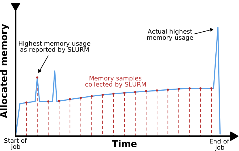
A graph plotting memory consumption of a job over time. The curve has an upwards trend with intermittent spikes. The periodic sampling of Slurm are shown as vertical lines intersecting the graph in regular intervals. While one of the memory spikes coincides with a sampling point, two others do not. One of them is near the start of the execution time and falls between two sample points. The other is at the very end of the execution time and occurs after the last sample point.

Caution

Slurm determines memory consuption by polling, i.e., periodically checking on the memory consumption of your job. If you job has a memory allocation profile with short spikes in memory usage, the value reported by seff can be incorrect. In particular, if the job gets cancelled due to memory exhaustion, you should not rely on the value reported by seff as it is likely significantly too low.

So how big is the peak memory consumption of our process really? Luckily, the Linux kernel keeps track of this for us, if Slurm is configured to use the so-called “cgroups v2” mechanism to enforce resource limits (which many HPC systems are). Let’s use this system to find out how much memory the raytracer actually needs. First, we set the memory limit back to 1 GB, i.e., to a configuration that is known to work.

BASH

#SBATCH --mem=1G

Next, add these lines at the end of your job script:

BASH

echo -n "Total amount of memory used (in bytes): "
CGROUPPATH="$(cat /proc/self/cgroup | awk -F ':' '{print $3}')"
cat /sys/fs/cgroup/${CGROUPPATH}/memory.peak

Let’s break down what each line does:

The first line prints out a nice label for our peak memory output. We use -n to omit the usual newline that echo adds at the end of its output.
For the next part we need the so-called “cgroup path” of our job. To find out this path, we can use the /proc/self/cgroup file, which contains this path as the third entry of a colon-separated list. Therefore, we read the contents of this file (cat) and extract the third entry of the colon-separated list (awk -F ':' '{print $3}'). Since we do this in $(...), Bash will place the output of these commands (i.e., the cgroup path) in the variable CGROUPPATH.
The third line outputs the contents of a file (cat). The path of this file starts with /sys/fs/cgroup, which is a location where the Linux kernel exports all the cgroups v2 information as files, followed by the cgroup path of our job in the CGROUPPATH variable.
The final part of the path is the information we actually want from the cgroup. In our case, we are interested in memory.peak, which contains the peak memory consumption of the cgroup.

When you submit your job and look at the output once it finishes, you will find a line like this:

OUTPUT

[...]
Total amount of memory used (in bytes): 579346432
[...]

So even though Slurm reported our job to only use 367.28 MB of memory, we actually used nearly 600 MB! With this measurement we can make an informed decision on how to set the memory limit for our job:

BASH

#SBATCH --mem=700M

Run your job again with this limit to verify that it completes successfully.

Callout

Too tight memory limits can reduce performance!

Slurm enforces memory limits for all processes in a job. Besides the applications memory demand (RSS - resident set size), this also includes caching mechanism of the Linux Kernel, e.g. for file I/O.

Too tight memory limits can cause too small caches next to the applications memory demand. This in turn can severely reduce the jobs performance in some cases.

Sizing your jobs: CPU Cores

So far we have tuned the time and memory limits of our job. Now let us have a look at the CPU core limit.

This limit works slightly differently than the ones we looked at so far in the sense that your job is not getting terminated if you try to use more cores than you have allocated. Instead, the scheduler exploits the fact that multitasking operating systems can switch out the process a given CPU core is working on. If you have more active processes in your job than you have CPU cores (i.e., CPU oversubscription), the operating system will simply switch processes in and out while trying to ensure that each process gets an equal amount of CPU time. This happens very fast, so you can’t see the switching directly, but tools like top will show your processes running at less than 100% CPU utilization.

Below you can see a situation of four processes running on three CPU cores, which results in each process running only 75% of the time.

Depicted is a situation of four processes running on three CPU cores, which results in each process running only 75% of the time.

Caution

CPU oversubscription can be harmful to performance as switching between processes by the operating system can cost a significant amount of CPU time itself.

Let’s try reducing the number of cores we allocate by reducing the number of MPI tasks we request in our job script:

BASH

#SBATCH --ntasks=2

Now we have a mismatch between the number of tasks we request and the number of tasks we use in mpirun. However, MPI catches our folly and prevents us from accidentally oversubscribing our CPU cores. In the output file you see the full explanation

OUTPUT

There are not enough slots available in the system to satisfy the 4
slots that were requested by the application:

  ./SnowmanRaytracer/build/raytracer

Either request fewer procs for your application, or make more slots
available for use.

A "slot" is the PRRTE term for an allocatable unit where we can
launch a process.  The number of slots available are defined by the
environment in which PRRTE processes are run:

  1. Hostfile, via "slots=N" clauses (N defaults to number of
     processor cores if not provided)
  2. The --host command line parameter, via a ":N" suffix on the
     hostname (N defaults to 1 if not provided)
  3. Resource manager (e.g., Slurm, PBS/Torque, LSF, etc.)
  4. If none of a hostfile, the --host command line parameter, or an
     RM is present, PRRTE defaults to the number of processor cores

In all the above cases, if you want PRRTE to default to the number
of hardware threads instead of the number of processor cores, use the
--use-hwthread-cpus option.

Alternatively, you can use the --map-by :OVERSUBSCRIBE option to ignore the
number of available slots when deciding the number of processes to
launch.

If we actually want to see oversubscription in action, we need to switch from MPI to multithreading. First, let us try without oversubscribing the CPU cores:

BASH

#SBATCH --ntasks=1
#SBATCH --cpus-per-task=4

# [...]

./SnowmanRaytracer/build/raytracer -width=1024 -height=1024 -spp=256 -threads=4 -alloc_mode=3 -png=snowman.png

We use the output of seff as a baseline for our multithreaded job:

OUTPUT

[...]
CPU Utilized: 00:21:32
CPU Efficiency: 99.08% of 00:21:44 core-walltime
Job Wall-clock time: 00:05:26
Memory Utilized: 90.85 MB
Memory Efficiency: 12.11% of 750.00 MB

Discussion

Challenge

Compare our measurements for 4 threads here to the measurements we made for doing the computation with 4 MPI tasks earlier. What metrics are similar and which ones are different? Do you have an explanation for this?

Show me the solution

We can see that the CPU utilization time and the walltime are virtually identical to the MPI version of our job, while the memory utilization is much lower. The exact reasons for this will be discussed in the following episodes, but here is the gist of it:

Our job is strongly compute-bound, i.e., the time our job takes is mostly determined by how fast the CPU can do its calculations. This is why it does not matter much for CPU utilization whether we use MPI or threads as long as both can keep the same number of CPU cores busy.
MPI typically incurs an overhead in CPU usage and memory due to the need to communicate between the tasks (in comparison, threads can share a block of memory without communication). In our raytracer, this overhead for CPU usage is negligible (hence the same CPU utilization time metrics), but there is a significant memory overhead.

Now let’s see what happens when we oversubscribe our CPU by doubling the number of threads without increasing the number of allocated cores in our job script:

BASH

./SnowmanRaytracer/build/raytracer -width=1024 -height=1024 -spp=256 -threads=8 -alloc_mode=3 -png=snowman.png

Discussion

Challenge

If you cluster allows direct access to the compute nodes, try logging into the node your job is running on and watch the CPU utilization live using

BASH

top -u <your username>

Compare the CPU utilization of the raytracter threads with different total numbers of threads.

In the top right of top you can also see a metric called load average. Simplified, this is the number of processes / threads that are currently either running or could run if a CPU core was free. Compare the amount of load you generate with your job depending on the number of threads.

Show me the solution

You can see that the CPU utilization of each raytracer thread goes down as the number of threads increases. This means, each process is only active for a fraction of the total compute time as the operating system switches between threads.

For the load metric, you can see that the load increases linearly with the number of threads regardless if they are actually running or waiting for a CPU core. Load is a fairly common metric to be monitored by cluster administrators, so if you cause excessive load by CPU oversubscription you will probably hear from your local admin.

Despite using twice the amount of threads, we barely see any difference in the output of seff:

OUTPUT

CPU Utilized: 00:21:29
CPU Efficiency: 98.85% of 00:21:44 core-walltime
Job Wall-clock time: 00:05:26
Memory Utilized: 93.32 MB
Memory Efficiency: 12.44% of 750.00 MB

This shows that despite having more threads, the CPU cores are not performing more work. Instead, the operating system periodically rotates the threads running on each allocated core, making sure every thread gets a time slice to make progress.

Let’s see what happens when we increase the thread count to extreme levels:

BASH

./SnowmanRaytracer/build/raytracer -width=1024 -height=1024 -spp=256 -threads=1024 -alloc_mode=3 -png=snowman.png

With this setting, seff yields

OUTPUT

CPU Utilized: 00:26:45
CPU Efficiency: 99.07% of 00:27:00 core-walltime
Job Wall-clock time: 00:06:45
Memory Utilized: 113.29 MB
Memory Efficiency: 15.11% of 750.00 MB

As we can see, our job is actually getting slowed down from all the switching between threads. This means, that for our raytracer application CPU oversubscription is either pointless or actively harmful regarding performance.

Discussion

Can you imagine a situation where CPU oversubscription might be sensible (perhaps also outside the HPC context)?

Show me the solution

On HPC we often have a CPU bound application, i.e., the work done by the CPU is the limiting factor and thus dividing this work into smaller chunks does not help with performance.

However, there are also applications bound by other resources. For these applications it makes sense to assign the CPU core elsewhere while the process is waiting, e.g., on a storage medium.

Also, on many systems it is desirable to have more programs running than your computer has CPU cores since often only a few of them are active at the same time. One common example is your everyday computer with multiple programs running at the same time.

Multi-node jobs

So far, we have only used a single node for our job. The big advantage of MPI as a parallelism scheme is the fact that not all MPI tasks need to run on the same node. Let’s try this with our Snowman raytracer example:

BASH

#!/bin/bash
#SBATCH --nodes=2
#SBATCH --partition=<put your partition here>
#SBATCH --ntasks=4
#SBATCH --cpus-per-task=1
#SBATCH --mem=700M
#SBATCH --time=00:07:00
#SBATCH --output=snowman-stdout.log
#SBATCH --job-name=snowman

# Always a good idea to purge modules first to start with a clean module environment
module purge
# <put the module load commands for your cluster here>

mpirun -- ./SnowmanRaytracer/build/raytracer -width=1024 -height=1024 -spp=256 -threads=1 -alloc_mode=3 -png=snowman.png

echo -n "Total amount of memory used (in bytes): "
CGROUPPATH="$(cat /proc/self/cgroup | awk -F ':' '{print $3}')"
cat /sys/fs/cgroup/${CGROUPPATH}/memory.peak

The important change here compared to the MPI jobs before is the --nodes=2 directive, which instructs Slurm to distribute the 4 tasks across exactly two nodes.

Callout

Slurm accepts ranges

You can also leave the decision of how many nodes to use up to Slurm by specifying a minimum and a maximum number of nodes, e.g.,

--nodes=1-3

would mean that Slurn can assign your job either one, two or three nodes.

Let’s look at the seff report of our job once again:

OUTPUT

[...]
Nodes: 2
Cores per node: 2
CPU Utilized: 00:21:32
CPU Efficiency: 98.78% of 00:21:48 core-walltime
Job Wall-clock time: 00:05:27
Memory Utilized: 280.80 MB
Memory Efficiency: 20.06% of 1.37 GB

We can see that Slurm did indeed split up the job such that each of the two nodes is running two tasks. We can also see that the walltime and CPU time of our job are basically the same as before. Considering the fact that communication between nodes is usually much slower than communication within a node, this result is surprising at first. However, we can find an explanation in the way our raytracer works. Most of the compute time is spent on tracing light rays through the scene for each pixel. Since these light rays are independent from one another, there is no need to communicate between the MPI tasks. Only at the very end, when the final image is assembled from the samples calculated by each task, there is some MPI communication happening. The overall communication overhead is therefore vanishingly small.

Callout

How well your program makes use of a larger number of nodes depends strongly on the amount of communication in your program.

We can also look at the memory consumption:

OUTPUT

[...]
Total amount of memory used (in bytes): 464834560
[...]

As we can see, there was indeed less memory consumed on the node running our submit script compared to before (470 MB vs 580 MB). However, our method of measuring peak memory consumption does not account for the second node. So let’s reach deeper into the toolbox to find out how much memory we actually use.

Tips for job submission

To end this lesson, we discuss some tips for choosing resource allocations such that your jobs get scheduled more quickly.

Many clusters have activated the so-called backfill scheduler option in Slurm. This mechanism tries to squeeze low priority jobs in the gaps between jobs of higher priority (as long as the larger jobs are not delayed by this). In this case, smaller jobs are generally advantageous as they can “skip ahead” in the queue and start early.
Using sinfo -t idle you can specifically search for partitions that have idle nodes. Consider using these partitions for your job if possible as an idle node will typically start your job immediately.
Different partitions might have different billing weights, i.e., they might use different factors to determine the “cost” of your calculation, which is subtracted from your compute budget or fairshare score. You can check these weights using scontrol show partition <partitionname> | grep TRESBillingWeights. The idea behind different billing weights is to even out the cost of the different resources (i.e., how many hours of memory use correspond to one hour of CPU use) and to ensure that using more expensive hardware carries an appropriate cost for the users.
Typically, it takes longer for a large slot to free up than it takes for several small slots to open. Splitting your job across multiple nodes might not be the most computationally efficient way to run it due to the possible communication overhead, but it can be more efficient in terms of scheduling.
Slurm produces an estimate on when your job will be started which you can check with scontrol show job 35749406 | grep StartTime.

Key Points

Your cluster might seem to have an enormous amout of computing resources, but these resources are a shared good. You should only use as much as you need.
Resource requests are a promise to the scheduler to not use more than a specific amount of resources. If you break your promise to the scheduler and try to use more resources, terrible things will happen.
- Overstepping memory or time allocations will result in your job being terminated.
- Oversubscribing CPU cores will at best do nothing and at worst diminish performance.
Finding the minimal resource requirements takes a bit of trial and error. Slurm collects a lot of useful metrics to aid you in this.

Content from Scheduler Tools

Last updated on 2026-08-13 | Edit this page

Overview

Questions

What can the scheduler tell about job performance?
What’s the meaning of collected metrics?

Objectives

After completing this episode, participants should be able to …

Explain basic performance metrics.
Use tools provided by the scheduler to collect basic performance metrics of their jobs.

Scheduler Tools

A scheduler performs important tasks such as accepting and scheduling jobs, monitoring job status, starting user applications, cleaning up jobs that have finished or exceeded their allocated time. The scheduler also keeps a history of jobs that have been run and how they behaved. The information that is collected can be queried by the job owner to learn about how the job utilized the resources it was given.

The `seff` tool

The seff command can be used to learn about how efficiently your job has run. The seff command takes the job identifier as an argument to select which job it displays information about. That means we need to run a job first to get a job identifier we can query SLURM about. Then we can ask about the efficiency of the job.

Callout

`seff` may not be available

seff is an optional SLURM tool for more convenient access to saact. It does not come standard with every SLURM installation. Your particular HPC system may or may not provide it. Check for it’s availability on your login nodes, or consult your cluster documentation or support staff.

Other third party alternatives, e.g. reportseff, can be installed with default user permissions.

The sbatch command is used to submit a job. It takes a job script as an argument. The job script contains the resource requests, such as the amount of time needed for the calculation, the number of nodes, the number of tasks per node, and so on. It also contains the commands to execute the calculations.

Using your favorite editor, create the job script render_snowman.sbatch with the contents below.

#!/usr/bin/bash
#SBATCH --time=01:00:00
#SBATCH --nodes=1
#SBATCH --tasks-per-node=4

# Possibly a "module load ..." command to load required libraries
# Depends on your particular HPC system

mpirun -np 4 raytracer -width=800 -height=800 -spp=128 -alloc_mode=3

Next submit the job with sbatch, and see what seff says about the job with the following commands.

BASH

jobid=$(sbatch --parsable render_snowman.sbatch)
seff $jobid

OUTPUT

Job ID: 309489
Cluster: bigiron
User/Group: usr123/grp123
State: COMPLETED (exit code 0)
Nodes: 1
Cores per node: 4
CPU Utilized: 00:07:43
CPU Efficiency: 98.93% of 00:07:48 core-walltime
Job Wall-clock time: 00:01:57
Memory Utilized: 35.75 MB
Memory Efficiency: 0.20% of 17.58 GB (4.39 GB/core)

The job script we created asks for 4 CPUs for an hour. After submitting the job script we need to wait until the job has finished as seff can only report sensible statistics after the job is completed. The report from seff shows basic statistics about the job, such as

The resources the job was given
- the number of nodes
- the number of cores per node
- the amount of memory per core
The amount of resources used
- CPU Utilized the aggregate CPU time (the time the job took times the number of CPUs allocated)
- CPU Efficiency the actual CPU usage as a percentage of the total available CPU capacity
- Job Wall-clock time the time the job took from start to finish
- Memory Utilized the aggregate memory usage
- Memory Efficiency the actual memory usage as a percentage of the total avaialable memory

Looking at the Job Wall-clock time it shows that the job took just under 2 minutes. Therefore this job took a lot less time than the one hour we asked for. This can be problematic as the scheduler looks for time windows when it can fit a job in. Long running jobs cannot be squeezed in as easily as short running jobs. As a result, jobs that request a long time to complete typically have to wait longer before they can be started. Therefore asking for more than 10 times as much time as the job really needs, simply means that you will have to wait longer for the job to start. On the other hand you do not want to ask for too little time. Few things are more annoying than waiting for a long running calculation to finish, just to see the job being killed right before the end because it would have needed a couple of minutes more than you asked for. So the best approach is to ask for more time than the job needs, but not go overboard here. As the job elapse time depends on many machine conditions, including congestion in the data communication, disk access, operating system jitter, and so on, you might want to ask for a substantial buffer. Nevertheless, asking for more than twice as much time as job is expected to need, usually doesn’t make sense.

Another thing is that SLURM by default reserves a certain amount of memory per core. In this case the actual memory usage is just a fraction of that amount. We could reduce the memory allocation by explicitly asking for less by modifying the render_snowman.sbatch job script.

Challenge

Edit the batch file to reduce the amount of memory requested for the job. Note that the amount of memory per node can be requested with the --mem= argument. The amount of memory is specified by a number followed by a unit. The units can represent kilobtytes (KB), megabytes (MB), gigabytes (GB). For the calculations we are doing here 100 megabytes per node is more than sufficient. Submit the job, and inspect the efficiency with seff. What is the memory usage efficiency you get?

Show me the solution

The batch file after adding the memory request becomes.

#!/usr/bin/bash
#SBATCH --time=01:00:00
#SBATCH --nodes=1
#SBATCH --tasks-per-node=4
#SBATCH --mem=100MB

# Possibly a "module load ..." command to load required libraries
# Depends on your particular HPC system

mpirun -np 4 raytracer -width=800 -height=800 -spp=128 -alloc_mode=3

Submit this jobscript, as before, with the following command.

BASH

jobid=$(sbatch --parsable render_snowman.sbatch)
seff $jobid

OUTPUT

Job ID: 310002
Cluster: bigiron
User/Group: usr123/grp123
State: COMPLETED (exit code 0)
Nodes: 1
Cores per node: 4
CPU Utilized: 00:07:43
CPU Efficiency: 98.09% of 00:07:52 core-walltime
Job Wall-clock time: 00:01:58
Memory Utilized: 50.35 MB
Memory Efficiency: 50.35% of 100.00 MB (100.00 MB/node)

The output of seff shows that about 50% of requested memory was used.

Now we see that a much larger fraction of the allocated memory has been used. Normally you would not worry too much about the memory request. Lately HPC clusters are used more for machine learning work loads which tend to require a lot of memory. Their memory requirements per core might actually be so large that they cannot use all the cores in a node. So there may be spare cores available for jobs that need little memory. In such a scenario tightening the memory allocation up could allow the scheduler to start your job early. How much milage you might get from this depends on the job mix at the HPC site where you run your calculations.

Note that the CPU utilization is reported as almost 100%, but this just means that the CPU was busy with your job 100% of the time. It does not mean that this time was well spent. For example, every parallel program has some serial parts to the code. Typically those parts are executed redundantly on all cores, which is wasteful but not reflected in the CPU efficiency. Also, this number does not reflect how well the capabilities of the CPU are used. If your CPU offers vector instructions, for example, but your code does not use them then your code will just run slow. The CPU efficiency will still show that the CPU was busy 100% of the time even though the program is just running at a fraction of the speed it could achieve if it fully exploited the hardware capabilities. It is worth keeping these limitations of seff in mind.

Callout

Good utilization does not imply efficiency

Measuring close to 100% CPU utilization does not say anything about how useful the calculations are. It’s merely stating, that the CPU was mostly busy with calculations, instead of waiting for data or running idle, waiting for other conditions to occur.

Good CPU utilization is only efficient, if it runs only “useful” calculations that contribute with new results towards an intended goal.

The seff command cannot give you any information about the I/O performance of your job. You have to use other approaches for that, and sacct may be one of them.

The `sacct` tool

The sacct command shows data stored in the job accounting database. You can query the data of any of your previously run jobs. Just like with seff you will need to provide the job ID to query the accounting database. Rather than keeping track of all your jobs yourself you can ask sacct to provide you with an overview of the jobs you have run.

BASH

sacct

OUTPUT

JobID           JobName  Partition    Account  AllocCPUS      State ExitCode
------------ ---------- ---------- ---------- ---------- ---------- --------
309902       render_sn+  STD-s-96h  project_a          4  COMPLETED      0:0
309902.batch      batch             project_a          4  COMPLETED      0:0
309902.exte+     extern             project_a          4  COMPLETED      0:0
309903       render_sn+  STD-s-96h  project_a          4  COMPLETED      0:0
309903.batch      batch             project_a          4  COMPLETED      0:0
309903.exte+     extern             project_a          4  COMPLETED      0:0
310002       render_sn+  STD-s-96h  project_a          4  COMPLETED      0:0
310002.batch      batch             project_a          4  COMPLETED      0:0
310002.exte+     extern             project_a          4  COMPLETED      0:0

In the output every job is shown three times here. This is because sacct lists one line for the primary job entry, followed by a line for every job step. A job step corresponds to an mpirun or srun command. The extern line corresponds to all work that is done outside of SLURM’s control, for example an ssh command that runs something somewhere else.

Note that by default sacct only lists the jobs that have been run today. You can use the --starttime option to list all jobs that have been run since the given start date. For example, try running

BASH

sacct --starttime=2025-09-25

OUTPUT

JobID           JobName  Partition    Account  AllocCPUS      State ExitCode
------------ ---------- ---------- ---------- ---------- ---------- --------
308755       snowman.s+  STD-s-96h  project_a         16  COMPLETED      0:0
308755.batch      batch             project_a         16  COMPLETED      0:0
308755.exte+     extern             project_a         16  COMPLETED      0:0
308756       snowman.s+  STD-s-96h  project_a          4  COMPLETED      0:0
308756.batch      batch             project_a          4  COMPLETED      0:0
308756.exte+     extern             project_a          4  COMPLETED      0:0
309486       interacti+  STD-s-96h  project_a          4     FAILED      1:0
309486.exte+     extern             project_a          4  COMPLETED      0:0
309486.0          prted             project_a          4  COMPLETED      0:0
309489       render_sn+  STD-s-96h  project_a          4  COMPLETED      0:0
309489.batch      batch             project_a          4  COMPLETED      0:0
309489.exte+     extern             project_a          4  COMPLETED      0:0
309902       render_sn+  STD-s-96h  project_a          4  COMPLETED      0:0
309902.batch      batch             project_a          4  COMPLETED      0:0
309902.exte+     extern             project_a          4  COMPLETED      0:0
309903       render_sn+  STD-s-96h  project_a          4  COMPLETED      0:0
309903.batch      batch             project_a          4  COMPLETED      0:0
309903.exte+     extern             project_a          4  COMPLETED      0:0
310002       render_sn+  STD-s-96h  project_a          4  COMPLETED      0:0
310002.batch      batch             project_a          4  COMPLETED      0:0
310002.exte+     extern             project_a          4  COMPLETED      0:0

You may want to change the date of 2025-09-25 to something more sensible when you work through this tutorial. Note that some HPC systems may limit the range of such a request to a maximum of, for example, 30 days to avoid overloading the slurm database with too large requests.

With the job ID you can ask sacct for information about a specific job as in

BASH

sacct --jobs=310002

OUTPUT

JobID           JobName  Partition    Account  AllocCPUS      State ExitCode
------------ ---------- ---------- ---------- ---------- ---------- --------
310002       render_sn+  STD-s-96h  project_a          4  COMPLETED      0:0
310002.batch      batch             project_a          4  COMPLETED      0:0
310002.exte+     extern             project_a          4  COMPLETED      0:0

Using sacct with the --jobs flag is just another way to select which jobs we want more information about. In itself it does not provide any additional information. To get more specific data we need to explicitly ask for the information we want. As SLURM collects a broad range of data about every job it is worth to evaluate what the most relevant items are.

MaxRSS, AveRSS, or the Maximum or Average Resident Size Set (RSS). The RSS is the memory allocated by a program that is actually resident in the main memory of the computer. If the computer gets low on memory then the virtual memory manager can extend the apparently available memory by moving some of the data from memory to disk. This is done entirely transparently to the application, but the data that has been moved to disk is no longer resident in main memory. As a result accessing it will be slower because it needs to retrieved from disk first. Therefore if the RSS is small compared to the total amount of memory the program uses this might affect the performance of the program.
MaxPages, AvePages, or the Maximum or Average number of Page Faults. These quantities are related to the Resident Size Sets. When the program tries to access data that is not resident in main memory this triggers a page fault. The virtual memory manager responds to a page fault by retrieving the accessed data from disk (and potentially migrating other data to disk to make space). These operations are typically costly. Therefore high numbers of page faults typically correspond to a significant reduction in the program’s performance. For example, the CPU utilization might drop from as high as 98% to as low as 2% due to page faults. For that reason some HPC machines are configured to kill your job if the application generates a high rate of page faults.
AllocCPUS is the number of CPUs allocated for the job.
Elapsed is the amount of wall clock time it took to complete the job. I.e. the amount of time that passed between the start and finish of the job.
MaxDiskRead, the Maximum amount of data read from disk.
MaxDiskWrite, the Maximum amount of data written to disk.
ConsumedEnergy, the amount of energy consumed by the job if that information was collected. The data may not be collected on your particular HPC system and is reported as 0.
AveCPUFreq, the average CPU frequency of all tasks in a job, given in kHz. In general the higher the clock frequency of the processor the faster the calculation runs. The exception is if the application is memory bandwidth limited and the data cannot be moved to processor fast enough to keep it busy. In that case modern hardware might throttle the frequency. This saves energy as the power consumption scales linearly with the clock frequency, but doesn’t slow the calculation down as the processor was having to wait for data anyway.

We can explicitly select the data elements that we are interested in. To see how long the job took to complete run

BASH

sacct --jobs=310002 --format=Elapsed

OUTPUT

   Elapsed
----------
  00:01:58
  00:01:58
  00:01:58

Challenge

Request information regarding all of the above variables from sacct, including JobID. Note that the --format flag takes a comma separated list. Also note that the result shows that more data is read than written, even though the program generates and write an image, and reads no data at all. Why would that be?

Show me the solution

To query all of the above variable run

BASH

sacct --jobs=310002 --format=MaxRSS,AveRSS,MaxPages,AvePages,AllocCPUS,Elapsed,MaxDiskRead,MaxDiskWrite,ConsumedEnergy,AveCPUFreq

OUTPUT

    MaxRSS     AveRSS MaxPages   AvePages  AllocCPUS    Elapsed  MaxDiskRead MaxDiskWrite ConsumedEnergy AveCPUFreq
---------- ---------- -------- ---------- ---------- ---------- ------------ ------------ -------------- ----------
                                                   4   00:01:58                                        0
    51556K     51556K      132        132          4   00:01:58        6.91M        0.72M              0         3M
         0          0        0          0          4   00:01:58        0.01M        0.00M              0         3M

Although the program we have run generates an image and writes that to a file, there is also a none zero amount of data read. The writing part is associated with the image file the program writes. The reading part is not associated with anything that the program does, as it doesn’t read anything from disk. It is instead associated with the fact that the operating system has to read the program itself and it’s dependencies to execute it.

Shortcomings

While seff and sacct provide a lot of information it is still incomplete. For example, the information is accumulated for the entire calculation. Variations in the metrics as a function of time throughout the job are not available. Communication between different MPI processes is not recorded. The collection of the energy consumption depends on the hardware and system configuration at the HPC center and might not be available. We are also often missing reliable measurements for I/O via the interconnect between nodes and the parallel file system.

So while we might be able to glean some indications for different types of performance problems, for a proper analysis more detailed information is needed.

Summary

This episode introduced the SLURM tools seff and sacct to get a high level perspective on a job’s performance. As these tools just use the statistics that SLURM collected on a job as it ran, they can always be used without any special preparation.

Challenge

So far we have considered our initial calculation using 4 cores. To run the calculation faster we could consider using more cores. Run the same calculation on 8, 16, and 32 cores as well. Collect and compare the results from sacct and see how the job performance changes.

Show me the solution

The machine these calculations have been run on has 112 core per node. So we can double the number of cores from 4 until 64 and stay within one node. If we go to two nodes then some of the communication between tasks will have to go across the interconnect. At that point the performance characteristics might change in a discontinuous manner. Hence we try to avoid doing that.

Alternatively you might scale the calculation across multiple nodes, for example 2, 4, 8, 16 nodes. With 112 cores per node you would have to make sure that the calculation is large enough for such a large number of cores to make sense.

Create running_snowmen.sh with

#!/usr/bin/bash
for nn in 4 8 16 32; do
    id=`sbatch --parsable --time=00:12:00 --nodes=1 --tasks-per-node=$nn --ntasks-per-core=1 render_snowman.sh`
    echo "ntasks $nn jobid $id"
done

Create render_snowman.sh with

#!/usr/bin/bash

# Possibly a "module load ..." command to load required libraries
# Depends on your particular HPC system

export START=`pwd`
# Create a sub-directory for this job if it doesn't exist already
mkdir -p $START/test.$SLURM_NTASKS
cd $START/test.$SLURM_NTASKS
# The -spp flag ensures we have enough samples per ray such that the job
# on 32 cores takes longer than 30s. Slurm by default is configured such
# that job data is collected every 30s. If the job finishes in less than
# that Slurm might fail to collect some of the data about the job.
mpirun -np $SLURM_NTASKS raytracer -width=800 -height=800 -spp 1024 -threads=1 -alloc_mode=3 -png=rendered_snowman.png

Next we submit this whole set of calculations

BASH

./running_snowmen.sh

producing

OUTPUT

ntasks 4 jobid 349291
ntasks 8 jobid 349292
ntasks 16 jobid 349293
ntasks 32 jobid 349294

After the jobs are completed we can run

BASH

sacct --jobs=349291,349292,349293,349294 \
      --format=MaxRSS,AveRSS,MaxPages,AvePages,AllocCPUS,Elapsed,MaxDiskRead,MaxDiskWrite,ConsumedEnergy,AveCPUFreq

to produce

OUTPUT

    MaxRSS     AveRSS MaxPages   AvePages  AllocCPUS    Elapsed  MaxDiskRead MaxDiskWrite ConsumedEnergy AveCPUFreq
---------- ---------- -------- ---------- ---------- ---------- ------------ ------------ -------------- ----------
                                                   4   00:09:35                                        0
   142676K    142676K        1          1          4   00:09:35        7.75M        0.72M              0       743K
         0          0        0          0          4   00:09:35        0.01M        0.00M              0      2.61M
                                                   8   00:05:01                                        0
   289024K    289024K        0          0          8   00:05:01       10.15M        1.45M              0       960K
         0          0        0          0          8   00:05:02        0.01M        0.00M              0      2.42M
                                                  16   00:02:21                                        0
   563972K    563972K       93         93         16   00:02:21       15.00M        2.94M              0      1.03M
         0          0        0          0         16   00:02:21        0.01M        0.00M              0      2.99M
                                                  32   00:01:14                                        0
  1082540K   1082540K      260        260         32   00:01:14       24.83M        6.07M              0      1.08M
         0          0        0          0         32   00:01:14        0.01M        0.00M              0         3M

Note that the elapse time goes down as the number of cores increases, which is reasonable as more cores normally can get the job done quicker. The amount of data read also increases as every MPI rank has to read the executable and all associated shared libraries. The volume of data written is harder to understand. Every run produces an image file rendered_snowman.png that is about 100KB in size. This file is written just by the root MPI rank. This cannot explain the increase in data written with increasing numbers of cores. The increasing number of page faults with increasing numbers of cores suggests that paging memory to disk is responsible for the majority of data written.

Key Points

Schedulers provide tools for a high level view on our jobs, e.g. sacct and seff
Important basic performance metrics we can gather this way are:
- CPU Utilization, often as fraction of time where CPU was active/elapsed time of the job
- Memory utilization, often measured as Resident Set Size (RSS) and number of Pages
sacct can also provide metrics about disk I/O and energy consumption
Metrics through sacct are accumulated for the whole job runtime and may be too broad for more specific insight

Content from Scaling Study

Last updated on 2026-08-13 | Edit this page

Overview

Questions

How many resources should be requested for a given job?
How does our application behave at different scales?
Will the application benefit from requesting more computational resources?

Objectives

After completing this episode, participants should be able to …

Perform a scaling study for a given application.
Notice different perspectives on scaling parameters.
Identify good working points for the job configuration.

At times, you may think: “The deadline is approaching too fast and we may not finish our project in time.” Maybe requesting more resources from our clusters scheduler does the trick? How could we know if it helps and by how much?

Answering this question is often a formal requirement for compute time requests at larger HPC systems. They want to see good scaling behavior in an application, before they give access to a bigger chunk of their computational power. So, how well does your parallel application utilize larger number of resources? How well, does it scale?

What is Scaling?

The execution time of parallel applications changes with the number of parallel processes or threads. For example, when keeping the problem size fixed, i.e. keep the same amount of calculations, running the application with more processes/threads typically results in shorter execution times. We will consider the problem size as fixed for the first sections of this episode and discuss the case of a varying problem size later.

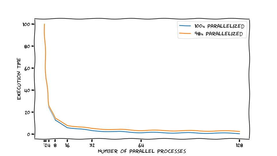
Sketched execution times for a perfectly and a 98% parallelized application. Doubling the number of parallel processors halves the execution time for the perfectly parallelized example, and a little bit less for the 98% parallelized version.

In a scaling study we measure how much a certain metric of an application, most commonly the execution time, changes with respect to the number of processes. In a common phrasing, this approach answers how the execution time scales with the number of parallel processors.

Starting from the job script render_snowman.sbatch:

BASH

#!/usr/bin/bash
#SBATCH --time=01:00:00
#SBATCH --nodes=1
#SBATCH --mem-per-cpu=200MB

# The `module load` command you had to load for building the raytracer
module load 2025 GCC/13.2.0 OpenMPI/4.1.6 buildenv/default Boost/1.83.0 CMake/3.27.6 libpng/1.6.40

time mpirun -- ./raytracer -width=800 -height=800 -spp=128 -png "$(date +%Y-%m-%d_%H%M%S).png"

we can manually run such a scaling study by submitting multiple jobs. In OpenMPI versions 4 and 5 the number of Slurm tasks is automatically picked up, so we do not set -n or -np of mpirun. We use -- to separate the arguments of mpirun (none in this case) from the MPI application raytracer and its arguments. Otherwise you may experience errors in some versions of OpenMPI 5, where mpirun misinterprets the arguments of raytracer as its own.

Callout

Scaling other resources with number of CPU cores

When scaling the resources outside of the job script, e.g. with sbatch --ntasks=X ..., as done above, we make sure to scale other resource requirements with the number of parallel processors. In this case, --mem-per-cpu=200MB is necessary to scale the amount of memory with the number of processors. --mem requests a fixed amount of memory per node.

For example, if each MPI process needs $100\,$MB, requesting $2\,$GB would only be enough for up to 20 MPI processes.

Forgetting a limit like this is a common pitfall in this situation.

Let’s start some measurements with $1$, $2$, $4$, and $8$ tasks:

OUTPUT

$ sbatch --ntasks 1 render_snowman.sbatch
Submitted batch job 16142767
$ sbatch --ntasks 2 render_snowman.sbatch
Submitted batch job 16142768
$ sbatch --ntasks 4 render_snowman.sbatch
Submitted batch job 16142769
$ sbatch --ntasks 8 render_snowman.sbatch
Submitted batch job 16142770

Now we have to wait until all four jobs are finished.

Callout

Regular update of `squeue`

You can use squeue --me -i 30 to get an update of all of your jobs every 30 seconds.

If you don’t need a more regular update, it is good practice to keep the interval on the order of 30s to a couple of minutes, just to be nice to Slurms server resources.

Once the jobs are finished, we can use grep "real" slurm-*.out to get the wall clock time of all four jobs:

OUTPUT

slurm-16142767.out:real       2m7.218s
slurm-16142768.out:real       1m7.443s
slurm-16142769.out:real       0m32.584s
slurm-16142770.out:real       0m17.480s

The real-time is decreasing significantly each time we double the number of Slurm tasks. From this, we feel that doubling the number of CPU cores really is a winning strategy!

Challenge

Exercise: Continue scaling study to larger values

Run the same scaling study and continue it for even larger number of --ntasks, e.g. 16, 32, 64, 128. So far, we have been using --nodes=1 to stay on a single node. At which point are your MPI processes distributed across more than one node? Use Slurm command line tools to find out the how many CPU cores (MPI processes) are available on a single node. You may have to increase the number of nodes with --nodes, if you want to go beyond that limit.

Gather your real time results and place them in a .csv file. Here is an example for our previous measurements:

ntasks,time
1,127.218
2,67.443
4,32.584
8,17.480
...

How much does each doubling of the CPU resources help with running the parallel raytracer?

Give me a hint

You can use sinfo to find out the node names of your particular Slurm partition. Then use scontrol to show all details about a single node from that partition. It will show you the number of CPU (cores) available on that node.

Show me the solution

ntasks,time
1,127.218
2,67.443
4,32.584
8,17.480
16,10.251
32,7.257
64,8.044
128,8.575

Using grep "real" slurm-*.out, we can see the execution time is halved in the beginning, with each doubling of the CPU cores. However, somewhere between $8$ and $16$ cores, we start to see less and less improvement.

Adding more resources does not help indefinitely. At some point the overhead of managing the calculation in separate tasks outweighs the benefit of parallel calculation. There is too little to do in each tasks and the overhead starts to dominate.

At some point adding more CPU cores does not help us anymore.

Adding more CPU cores can actively slow down the calculation after a certain point. The optimal point is different for each application and each configuration. It depends on the ratio between calculations, communications and various management overheads in the whole process of running everything.

Callout

Overheads and Reliable Measurements

Many overheads and when they show also depend on the underlying hardware. So the sweet spot may very well be different for different clusters, even if the application and configuration stays the same! For example, network communication always introduces latencies (short waiting times) for each connection and their bandwidth determines how long a communication takes. Here, clusters using different network architectures and technologies often exhibit different scaling behavior and configuration sweet spots for your applications.

Another common issue lies within our measurements themself. We perform a single time measurement on a worker node that is possibly shared with other jobs at the same time. What if another user runs an application that hogs shared resources like the local disk or network interface card? In this case our measurements become somewhat non-deterministic. Running the same measurement twice may result in significantly different values. If you need reliable results, e.g. for a publication, requesting exclusive access to Slurms resources through the sbatch flag --exclusive is the best approach. As a drawback, this typically results in longer waiting times, since whole nodes have to be reserved for the measurement jobs, even if not all resources are used.

Even on exclusive resources, the measurements cannot be 100% reliable. For example, the scheduling behavior of the Linux kernel, or access to remote resources like the parallel file system or data from the web, are still affecting your measurements in unpredictable ways. Therefore, the best results are achieved by taking the mean and standard deviations of repeated measurements for the same configuration. The measured minimum also has strong informative value, since it proofs the best observed behavior.

Keep in mind, --exclusive will always request all resources of a given node, even if only few cores are used. In these cases, tools like seff show worse resource utilization results, since measurements are done with respect to all booked resources.

Scaling studies can also be done with respect to different application and job parameters. For example, what is the execution time when we change the workload, e.g. a larger number of pixels, samples per pixels, or a more complex scene? How much does a communication overhead change, if we change the number of involved nodes while keeping the workload and number of tasks fixed, i.e. changing the network communication surface? Scaling studies like these can help identify pressure points that affect the applications performance.

Scaling studies typically occur in a preparation phase where the application is evaluated with a representative example workload. Once a good configuration is found, we know the application is running close to an optimal performance and larger number of calculations can start, often called the production phase.

In a similar vein, scaling studies can be a formal requirement for compute time applications on larger HPC systems. On these systems and for larger calculation campaigns it is more crucial to run efficient calculations, since the resources are typically more contested and the potential energy- and carbon footprint becomes much larger.

Speedup, Efficiency, and Strong Scaling

To quantitatively and empirically study the scaling behavior of a given application, it is common to look at the speedup and efficiency with respect to adding more parallel processors.

Speedup is a metric to compare the execution times with different amounts of resources. It answers the question

How much faster is the application with $N$ parallel processes/threads, compared to the serial execution with $1$ process/thread)?

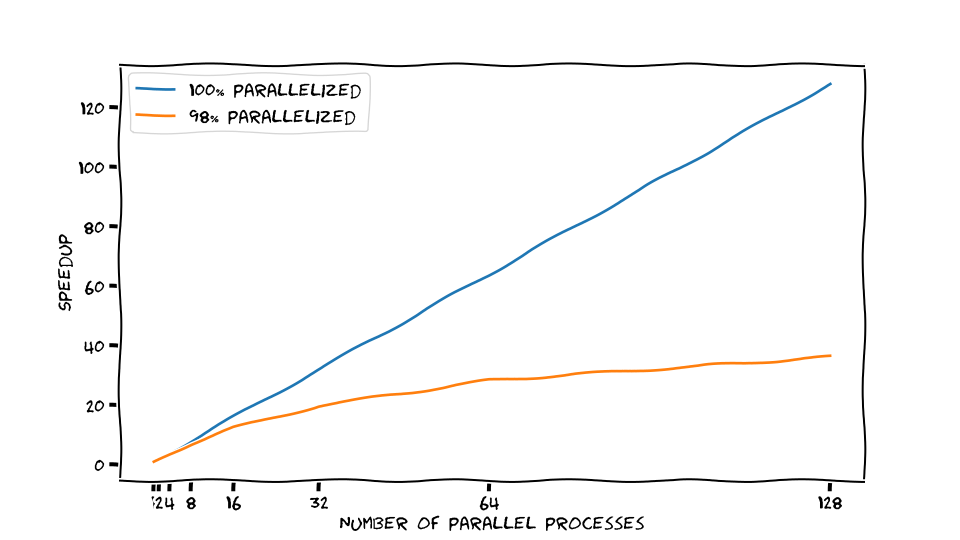
Sketched speedup for a perfectly and 98% parallelized application. Doubling the number of parallel processors makes the perfectly parallel application twice as fast. The 98% parallelized application does not speed up at the same rate.

Speedup is defined by the comparison of wall times $T(N)$ of the application with $N$ parallel processes: \[S(N) = \frac{T(1)}{T(N)}\] Here, $T(1)$ is the wall time for a sequential execution, and $T(N)$ is the execution with $N$ parallel processes. For our raytracer, with $2$ processes, we observe a speedup of $S(2) = \frac{127.218}{67.443} \approx 1.89$ In reality, our application only got $1.89\times$ faster, for the $2$ parallel processes we have spent on it. Ideally, we would have expected a speedup of $2$, so our application does not seem perfectly efficient in terms of using the additional parallel processes to be faster.

We can calculate the efficiency with wich each additional parallel process contributes to the applications speedup: \[\eta(N) = \frac{S(N)}{N}\]

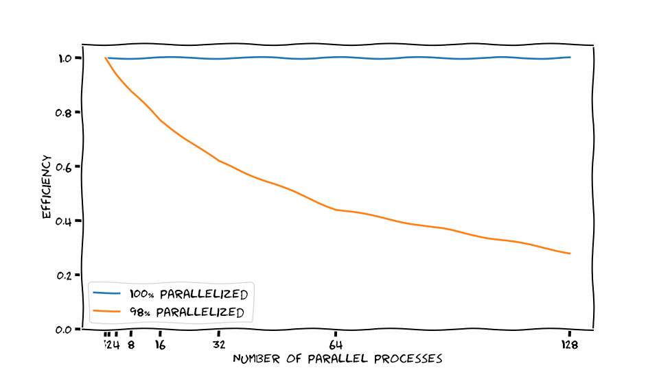
Sketched efficiency for a perfectly and 98% parallelized application. For the perfectly scaling case, each additional parallel process contributes well to solving the calculations faster. For the 98% parallelized application, adding more parallel processes has diminishing returns.

Challenge

Exercise: Calculate Speedup and Efficency

Extend the .csv file of your measurements from above with a speedup and efficiency column. It may look like this:

ntasks,time,speedup,efficiency
1,127.218,1.00,1.00
2,67.443,1.89,0.94
4,32.584,3.90,0.98
8,17.480,7.28,0.91
...

You may want to use any data visualization tool, e.g. python or spreadsheets, to visualize the data.

What number of processes may be a good working point for the raytracer with $800 \times 800$ pixel and $128$ samples per pixel?

Show me the solution

For all of our measurements, the speedup and efficiencies are

ntasks,time,speedup,efficiency
1,127.218,1.00,1.00
2,67.443,1.89,0.94
4,32.584,3.90,0.98
8,17.480,7.28,0.91
16,10.251,12.41,0.78
32,7.257,17.53,0.55
64,8.044,15.82,0.25
128,8.575,14.84,0.12

Plotting the speedup and efficiency helps with identifying a good working point:

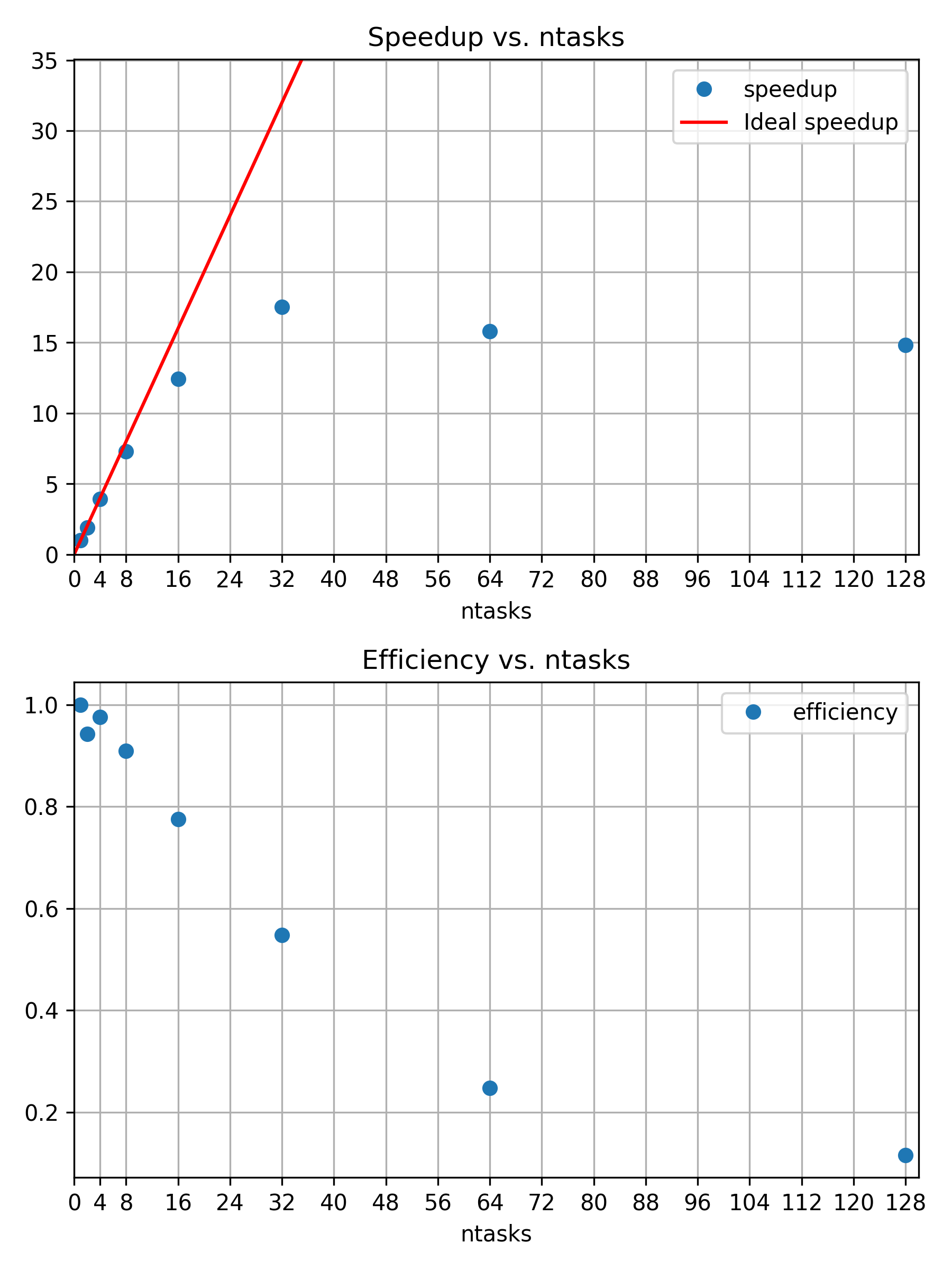
Speedup and efficiency of strong scaling example

The 16th processor is still close to 80% efficient. The corresponding speedup is less than the theoretical optimum, which is visualized by a red line of slope $1$.

There is no exact optimum and the best working point is open for discussion. However, it would be difficult to justify additional cores, if their contribution to speedup is only 50% efficient or even less.

Discussion

Discussion: Why does the Speedup Efficiency drop?

Adding more and more resources is not always speeding up our application. What may be possible reasons for worse speedup efficiency at larger numbers of parallel processors/threads?

Briefly collect and discuss any reasons you can think of.

(Optional) plotting our .csv

If you have experience with python, you can use our python script to create the same plots as above, but for your own data. It depends on numpy, pandas, and matplotlib, so make sure to prepare a corresponding python environment.

The script expects your .csv files to be called strong.csv and weak.csv, and be placed in the same directory.

So far, we kept the workload size fixed to $800 \times 800$ pixels and $128$ samples per pixel for the same scene with three snowman. The diminishing returns for adding more and more parallel processors leads to a famous observation. The speedup of a program through parallelization is limited by the execution time of the serial fraction that is not parallelizable. No application is 100% parallelizable, so adding an arbitrary amount of parallel processors can only affect the parallelizable section. In the best case, the execution time gets reduced to the serial fraction of the application.

An application is said to scale strongly, if adding more cores significantly reduces the execution time.

Callout

Amdahls Law¹

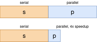
The model behind Amdahls Law: Assume an application consists of serial sections, e.g. reading from a file, and parallelizable sections, e.g. calculations in a loop. Both fractions add up to the whole program, i.e. $s + p = 1$. Here, Speedup through parallelization is inherently limited by only speeding up the parallel sections.

The speedup of a program through parallelization is limited by the execution time of the serial fraction that is not parallelizable. For a given execution time $T(N) = s + \frac{p}{N}$, with $s$ the serial fraction, and $p$, the parallel fraction of the applications execution time, speedup $S$ is defined as \[S(N) = \frac{T(1)}{T(N)} = \frac{1}{s + \frac{p}{N}} \Rightarrow \lim_{N\rightarrow \infty} S(N) = \frac{1}{s}\]

In other words, increasing the number of parallel processes $N$ for an application that only has a serial part that is taking up $1$% of the execution time, will never exceed a speedup of $\frac{1}{s} = \frac{1}{0.01} = 100$. No matter how many processes we will use!

Discussion

Discussion: When should we stop adding CPU cores?

Discuss your previous results and decide on a good working point. How many cores are still usefully reducing the execution time.

What other factors could affect your decision, e.g. available hardware and corresponding waiting times.

If scaling is limited, why are there larger HPC systems? Weak scaling.

For a fixed problem size, we observed that adding more parallel processors can only help up to a certain point. But what if the project benefits from increasing the workload size, i.e. doing more calculations? For example, does a higher resolution, more accuracy, or more statistics, etc., improve our insights and results? In this case, our perspective on efficiency changes and we address a different optimization than before: Doing more calculations with an increasing number of parallel processors. For our raytracer example, increasing the workload corresponds to more pixels, more samples per pixel, and/or a more complex scene.

Weak scaling refers to the scaling behavior of an application for a fixed workload per parallel processing unit, e.g. increasing the number of pixels by the same amount as the number of parallel processors $N$.

Callout

The difference between strong and weak scaling

In the previous discussion about Amdahls Law we kept the total amount of calculations fixed and increased the number of parallel processors $N$. Now, we are transitioning to a different perspective where we increase both, the number total amount of calculations and the number of parallel processors $N$,

In the former, we reach an absolute limit for moderate numbers of $N$ and would not benefit from increasing the number of parallel processes $N$. In the later case, we may benefit solving more calculations and we hope to be back in the business of Supercomputers with an $N$ in the order of thousands!

To scale the workload of the snowman raytracer, we can increase the number of calculated pixels with the same factor with which we increase the number of parallel processors. For one processor we have $800 \times 800 = 640000$ pixel. That means for two processors we need a height and a width of $\sqrt{2 \times 640000} = 1131.371 \approx 1131$. And similarly increasing the number of pixels for $--ntasks=4$ and so on.

The job script could look like this:

BASH

#!/usr/bin/bash
#SBATCH --time=01:00:00
#SBATCH --nodes=1
#SBATCH --mem-per-cpu=3800MB

module load 2025 GCC/13.2.0 OpenMPI/4.1.6 buildenv/default Boost/1.83.0 CMake/3.27.6 libpng/1.6.40

# Create associative array
declare -A pixel
pixel[1]="800"
pixel[2]="1131"
pixel[4]="1600"
pixel[8]="2263"
pixel[16]="3200"
pixel[32]="4526"
pixel[64]="6400"

time mpirun -- ./build/raytracer -width=${pixel[${SLURM_NTASKS}]} -height=${pixel[${SLURM_NTASKS}]} -spp=128 -threads=1 -png "$(date +%Y-%m-%d_%H%M%S).png"

Different ways of scaling workloads: spp

In each scaling study, it is crucial to identify which application parameters affect the execution time. There are often multiple ways.

For the snowman raytracer, instead of changing the total number of pixels, we can multiply the number of parallel MPI processes (${SLURM_NTASKS}) with the samples per pixel (starting from -spp=128). For a single process, the whole $800 \times 800$ pixel picture is calculated in a single MPI process with 128 per pixel. Running with two MPI processes, both have to calculate half the number of pixels, but twice the amount of samples per pixel.

BASH

#!/usr/bin/bash
#SBATCH --time=01:00:00
#SBATCH --nodes=1
#SBATCH --mem-per-cpu=500MB

module load 2025 GCC/13.2.0 OpenMPI/4.1.6 buildenv/default Boost/1.83.0 CMake/3.27.6 libpng/1.6.40

SPP="$[${SLURM_NTASKS}*128]"

time mpirun -- ./build/raytracer -width=800 -height=800 -spp=${SPP} -threads=1 -png "$(date +%Y-%m-%d_%H%M%S).png"

Three snowmen in 800x800 with 128 samples per pixel

Three snowmen in 800x800 with 8192 samples per pixel

In direct comparison, and zooming in really close, you can see more noise in Figure 1, e.g. in the shadows, relative to Figure 2. One could argue that we passed the point of diminishing returns, though. Is a $64\times$ increase in computational cost worth the observed quality improvement? For the samples per pixel, we seem to not benefit much from weak scaling. Larger resolutions, by increasing the number of pixels, may be a more useful dimension to increase in this case.

The usefulness of any computation can only be determined in the context of your scientific goals.

Increasing the resolution may be worth the effort, if we have a use for a larger, more detailed picture. In practice, there is a cutoff, beyond which no reasonable improvement is to be expected. This is a question about accuracy, error margins, and overall quality, which can only be answered in the specific context of each research project. If there is no tangible benefit of increasing the workload, running at a larger number of parallel processes does not serve a purpose, even if the application still exhibits good “weak scaling efficiency”.

If we increase the workload at the rate as our number of parallel processes ($N$) our speedup is defined as \[S_{\text{weak}}(N) = \frac{T(1)}{T(N)} \times N\] since we do $N$ times more work with $N$ processors, compared to our reference $T(N=1)$. Efficiency is still defined as \[\eta_{\text{weak}}(N) = \frac{S_{\text{weak}}(N)}{N} = \frac{T(1)}{T(N)}\]

Challenge

Exercise: Weak scaling

Repeat the previous scaling study and increase the number of pixels accordingly to study the raytracers weak scaling behavior.

Run with 1, 2, 4, 8, 16, 32, 64 MPI processes on single node
Take time measurements and consider running with --exclusive to ensure more reliable results.
Create a .csv file and run the plotting script

ntasks, pixel,    time, speedup, efficiency
     1,   800, 123.162,     ???,        ???
     2,  1131, 122.562,     ???,        ???
     4,  1600,     ???,     ???,        ???
     8,  2263,     ???,     ???,        ???
...

How well does the application scale with an increasing workload size? Do you see a qualitative difference in the resulting .png files and is the increased sample-per-pixel size worth the computational costs?

Show me the solution

ntasks, pixel,    time, speedup, efficiency
     1,   800, 123.162,    1.00,       1.00
     2,  1131, 122.562,    2.01,       1.00
     4,  1600, 124.522,    3.96,       0.99
     8,  2263, 125.606,    7.84,       0.98
    16,  3200, 125.803,   15.66,       0.98
    32,  4526, 130.137,   30.28,       0.95
    64,  6400, 138.636,   56.86,       0.89

The scaling behavior is reaching an asymptotic limit, where each additional processor is contributing with the same efficiency to the increased workload.

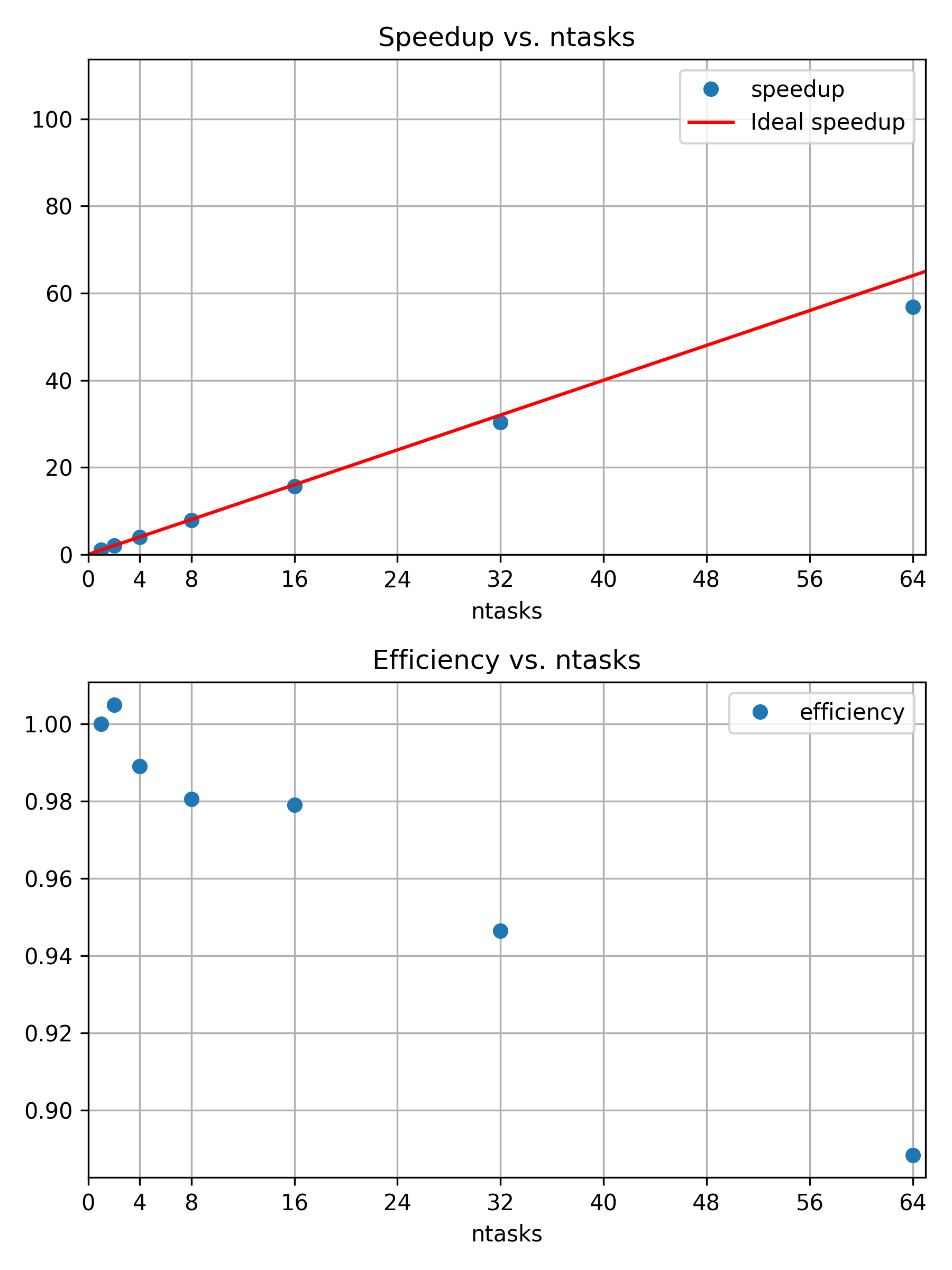
Speedup and efficiency of weak scaling example

Weakly scaling jobs can make efficient use of a huge amount of resources.

The most important question is, if an increased workload is producing useful results. Here, we have the rendered picture of three snowmen in 800x800 with 128 samples per pixel and three snowmen in 6400x6400 with 128 samples per pixel. The second image has a much higher resolution. However, going way beyond $6400 \times 6400$ pixels is probably not very meaningful, unless you are trying to print the worlds largest ad boards or similar.

Callout

Gustafsons Law²

A program scales on $N$ parallel processors, if the problem size also scales with the number of processors. The speedup $S$ becomes \[\text{S(N)} = \frac{s+pN}{s+p} = s+pN = s+(1-s)N\] with $N$ processors, $s$ the serial fraction, and $p$ the parallel fraction of the execution time.

Summary

In this episode, we have seen that we can study the scaling behavior of our application with respect to different metrics, while varying its configuration. Most commonly, we study the execution time of an application with an increasing number of parallel processors. In such a scaling study, we collect comparable walltime measurements for an increasing number of Slurm tasks of a parallelizable and representative job. If a good working point is found, larger scale “production” jobs can be submitted to the HPC system.

If the application has good strong scaling behavior, adding more cores leads to an effective improvement in execution time. We observe diminishing returns of adding more cores to a fixed-size problem, so there is a (subjective) optimal number of parallel processors for a given application configuration. (Amdahls Law)

If increasing the workload size leads to better results, maybe because of improved accuracy and quality, we can study the weak scaling behavior and increase the workload size by the same factor of increasing parallel processors.

A good working point depends on the availability of resources, specifics of the underlying hardware, the particular application, and a particular configuration for the application. For that reason, scaling studies are a common requirement for formal compute time applications to prove an efficient execution of a given application.

We can study the impact of any parameter on metrics like, for example, walltime, CPU utilization, FLOPS, memory utilization, communication, output size on disk, and so on.

Automating Scaling Studies

If you find yourself repeating similar measurements over and over again, you may be interested in an automation approach. This can be done by creating reproducible HPC workflows using JUBE, among other things.

Up to now, we were still working with basic metrics like the wall-clock time. In the next episode, we start with more in-depth measurements of many other aspects of our job and application.

Key Points

Jobs behave differently with increasing parallel resources and fixed or scaling workloads
Scaling studies can help to quantitatively grasp this changing behavior
Good working points are defined by configurations where more cores still provide sufficient speedup or improve quality through increasing workloads
Amdahl’s law: speedup is limited by the serial fraction of a program
Gustafson’s law: more resources for parallel processing still help, if larger workloads can meaningfully contribute to project results

G. M. Amdahl, ‘Validity of the single processor approach to achieving large scale computing capabilities’, in Proceedings of the April 18-20, 1967, spring joint computer conference, in AFIPS ’67 (Spring). New York, NY, USA: Association for Computing Machinery, Apr. 1967, pp. 483–485. doi: 10.1145/1465482.1465560.↩︎
J. L. Gustafson, ‘Reevaluating Amdahl’s law’, Commun. ACM, vol. 31, no. 5, pp. 532–533, May 1988, doi: 10.1145/42411.42415.↩︎

Content from Performance Overview

Last updated on 2026-08-13 | Edit this page

Overview

Questions

Is job wall-time the only way to study job performance?
What are commonly used metrics to describe job performance?
What are common workflows to evaluate performance?
How can I find the bottlenecks in a given job?

Objectives

After completing this episode, participants should be able to …

Create a comprehensive performance overview through dedicated tools.
Explain the difference between sampling and tracing.
Measure utilization and the impact of underlying hardware components.
Determine if their job is affected by a typical performance bottleneck pattern.

Wall-time measurements with time do not tell us why exactly an application is slower than expected. To learn more about the why, we have to measure our applications behavior in more detail and capture the utilization of underlying hardware.

Callout

The performance measurement tool

ClusterCockpit: A job monitoring service available on many clusters in NRW. Sampled measurements of the application are stored and visualized in a timeline for each job. It needs to be centrally provided by your HPC administration team and may not be available to you!

This tool may require access to performance counters, sometimes granted by requesting --exclusive, but it really depends on the system. If something covered in this episode isn’t available or looks different on your cluster, check your cluster documentation or ask your HPC support staff.

Let us set up our performance measurement tool by running an example job with 8 cores. To give the job enough work to be worth measuring, let’s go with $2263 \times 2263$ pixels and -spp=512, we repeat this experiment twice back to back.

A single run finishes quickly and would give ClusterCockpit only a handful of samples to plot, making the timelines look sparse and hard to read. Running it twice stretches the job out to a longer time, giving the sampling-based collectors enough time to gather a richer set of data points, which makes for much clearer plots when we look at the metrics. Additionally, we limit the execution time to 20 minutes to not wait too long, before getting the results. It does not hurt us, if the job gets cut off by the Slurm TIMEOUT, since the measurements will still represent the applications behavior up to that point.

Submit a job that runs for at least $5$ minutes, so it is picked up by cluster cockpit. The job could look like this:

BASH

#!/usr/bin/bash
#SBATCH --time=00:20:00
#SBATCH --partition=intelsr_devel
#SBATCH --ntasks=4
#SBATCH --cpus-per-task=1
#SBATCH --nodes=1
#SBATCH --exclusive

module purge
module load GCC/13.2.0 OpenMPI/4.1.6-GCC-13.2.0 CMake/3.27.6-GCCcore-13.2.0 Boost/1.83.0-GCC-13.2.0 libpng/1.6.40-GCCcore-13.2.0

for i in {1..3}; do
    mpirun -- ./build/raytracer -width=2263 -height=2263 -spp=512 -threads=1 -png "img_${SLURM_JOB_ID}_$(date +%Y-%m-%d_%H%M%S).png"
done

We will call this job 1. Note the use of --exclusive here, which books a whole node for the job. This is important to make sure the performance measurements are not disturbed by concurrent jobs. Additionally, ClusteCockpit collects some metrics only on a per-node basis, so concurrent jobs would make these measurements less usable

Discussion

Exercise: Run a second job with `raytracer_float4`

Submit a second job using the raytracer_float4 executable instead of raytracer — keep the resolution, -spp, core count, repeat count, and --exclusive request all the same as the original job.

We will call this job 2.

Show me the solution

There are other binaries next to the raytracer example, called raytracer_float4, _float8, _float16. We can start one of those in our job script instead:

BASH

#!/usr/bin/bash
#SBATCH --time=00:20:00
#SBATCH --partition=intelsr_devel
#SBATCH --ntasks=4
#SBATCH --nodes=1
#SBATCH --cpus-per-task=1
#SBATCH --exclusive

module purge
module load GCC/13.2.0 OpenMPI/4.1.6-GCC-13.2.0 CMake/3.27.6-GCCcore-13.2.0 Boost/1.83.0-GCC-13.2.0 libpng/1.6.40-GCCcore-13.2.0

for i in {1..3}; do
    mpirun -- ./build/raytracer_float4 -width=2263 -height=2263 -spp=512 -threads=1 -png "$(date +%Y-%m-%d_%H%M%S).png"
done

While the test jobs are running, let’s look into the relationship between computer hardware architecture and performance.

Hardware Architecture & Counters

Broadly categorized, a jobs performance is mostly dependent on

CPU utilization, e.g. how quickly instructions can be send to the processor, how quickly and how much data can be read from memory, and the raw calculation capabilities of the CPU.
Memory utilization may vary in terms of how much data is stored in memory, how often data in memory is written or read, and how quickly the data can be read and written to.
Disk input and output affects jobs that work with amounts of data that exceed available memory capacities.
Network input and output affects applications that rely on remote data, e.g. MPI applications that regularly share results between processes on multiple worker nodes.

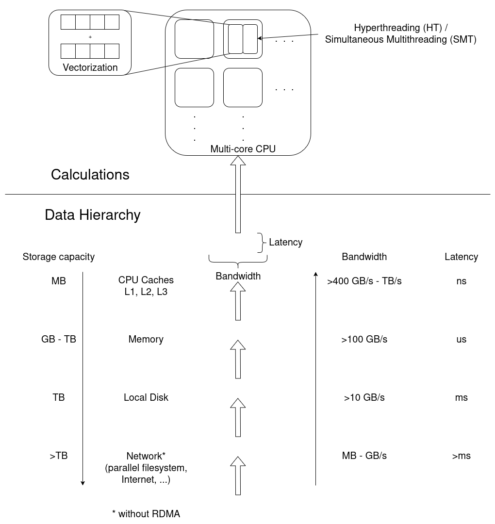
Diagram to visualize the data hierarchy of CPU architectures. Network, local disks, memory, and CPU caches have decreasing amounts of storage capacity, but increasing bandwidths and shorter latencies. Calculations occur in CPUs, possibly in multiple CPU cores, which may have multiple threads each, and even apply vectorized instructions.

Measurement Workflows

To learn how applications utilize the computers hardware, we employ third party tools that read usage metrics from performance counters, often implemented either in the operating system kernels (software) or in hardware.

Dedicated performance measurement tools often employ similar methods and rely on the same sources of information, but they my focus on different issues and use different data processing and visualization methods.

In general there are two approaches to performance measurements:

Sampling: Read out performance counters and the application state at regular intervals during execution
Tracing: Record every event and operation that occurs

Tracing is exact and allows for a very detailed analysis. On the other hand, it results in very large amounts of measurement data that even affects the applications performance during data collection. It may be impractical in some situations.

Sampling on the other hand is less exact and results in a statistical description of the applications behavior. Sampling has a smaller measurement overhead, but may suffer from, for example, slight mis-attributions of measurements to wrong sections of the code and fluctuating results between repeated measurements.

Measurement results are either stored and analysed in a timeline, or aggregated into a final measurement, often called a profile.

General Report

Going back to our Cluster Cockpit results, log in to the ClusterCockpit web interface of your HPC system, as explained in your cluster documentation. Go to My Jobs and click on the job 1 with the same Slurm job id, once it is available

"My Jobs" tab in the ClusterCockpit web UI

As a first step, to go beyond a wall-time analysis, we employ the measurement tool to produce a general overview of our applications behavior. Here, we typically try to answer questions like:

Are available CPU, memory, disk, and network capabilities utilized well?
Dose the jobs performance depend on a particular hardware component?
Is there an obvious contention point that could be eliminated?

First Overview

The job view of a particular job in ClusterCockpit begins with three summary panels for the job.

The Job Info panel summarizes Slurm metadata about the job, e.g. job ID, accounts, start time, duration, etc.

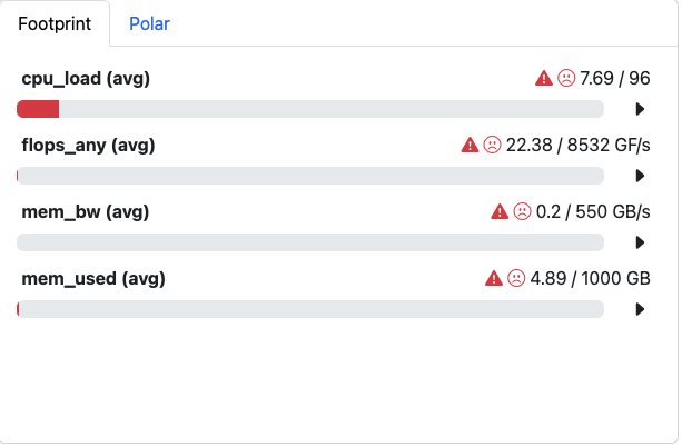
Cluster Cockpit Footprint panel summarizing central job characteristics

The Footprint panel summarizes a preconfigured set of performance characteristics for the job. It categorizes values in a traffic-light system, so yellow and red indicators motivates further investigation. The exact list and type of metrics depends on the ClusterCockpit configuration, which is prepared by the administrator of the service.

Here, all four values are not in acceptable range. We see why:

cpu_load (avg) is shown in red. Since we requested the node with --exclusive, we were given all $96$ cores of the node, but our job only uses $8$ of them. The footprint compares load against the full $96$ cores that are requested by us, so it correctly flags that most of the requested resources are sitting idle. This is underutilization of requested resources.
flops_any (avg) is Floating Point Operations per second. In this case, it is calculated as $22.38 GF/s$, which is far below what the node can theoretically achieve. It can point to anything from not utilizing the hardware features to simply not needing many floating point operations at all.
mem_used (avg) shows the memory utilization of the job. This, together with the bandwidth metric below, is exactly why we requested an exclusive node in the first place: memory- and energy-related hardware counters are not available at a per-core granularity. They are measured at socket level or node level rather than per core, so running exclusively is what keeps them meaningful for our job alone.
mem_bw (avg) is the memory bandwidth, i.e. how much data is transferred to and from memory per second.

Callout

Granularity of Metrics

Not every metric ClusterCockpit shows describes your job. Some describe the whole CPU socket, or even the whole node, regardless of how many cores your job actually occupies. The underlying collectors read hardware performance counters that are simply wired up at a particular level of the machine, and they have no notion of which Slurm job is currently running. This is true regardless of which monitoring tool you use, but it is essential to understand for reading ClusterCockpit correctly.

Metrics come in three granularities:

Core-level: measured separately for each individual CPU core, e.g. cpu_user, ipc, flops_any. These are meaningful for your job even if other jobs share the same node, since each core is attributed to exactly one job.
Socket-level: measured once for an entire CPU socket (which may host several cores of several different jobs), e.g. mem_bw and the package power reading behind the Energy panel (pkg_pwr). If another job shares your socket, its memory traffic or power draw is mixed into your measurement.
Node-level: measured once for the whole compute node, e.g. cpu_load, mem_used and network or filesystem metrics. These are effected by every job on the node, not just yours.

Each metric plot in ClusterCockpit has a small drop-down menu as shown in image below, typically labelled core, socket, or node. This label tells you directly at which granularity that particular chart was measured — a core selection means one line per core of your job, while socket or node means the value is shared with (and possibly polluted by) other jobs. If the drop-down only offers socket or node, treat the value with more caution unless you know the node was exclusively yours

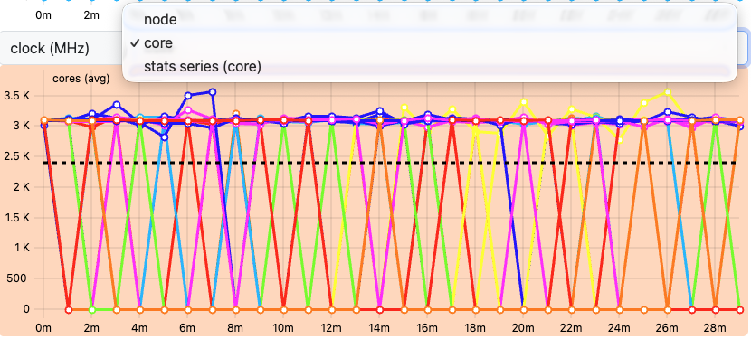
This is precisely why we requested --exclusive when submitting our job earlier in this episode: on a node reserved exclusively for our job, socket- and node-level metrics describe our job alone, since there is nothing else running to mix into the measurement. If you cannot use --exclusive, for example because your allocation only ever needs a fraction of a node, keep an eye on which granularity a given metric is measured at, and treat socket- or node-level values as an upper bound that may include other jobs’ activity rather than a precise reading of your own.

Select Metrics button in the ClusterCockpit job view

More detailed plots for each individual metric are available and can be configured through the Select Metrics button.

In general, the footprint panel gives the most information on what issues our job may have and where to start the investigation. In our case:

We can utilize all $96$ cores instead of just $8$ to make use of the full exclusive allocation.
We can try to improve either flops_any or mem_bw. To know which one actually makes sense to target, we need to look at the next panel, the Roofline plot.

How to read a Roofline Plot

Before looking at our job’s result, here’s what to expect on Roofline plot and how to understand the plot. Here is the example Roofline Plot:

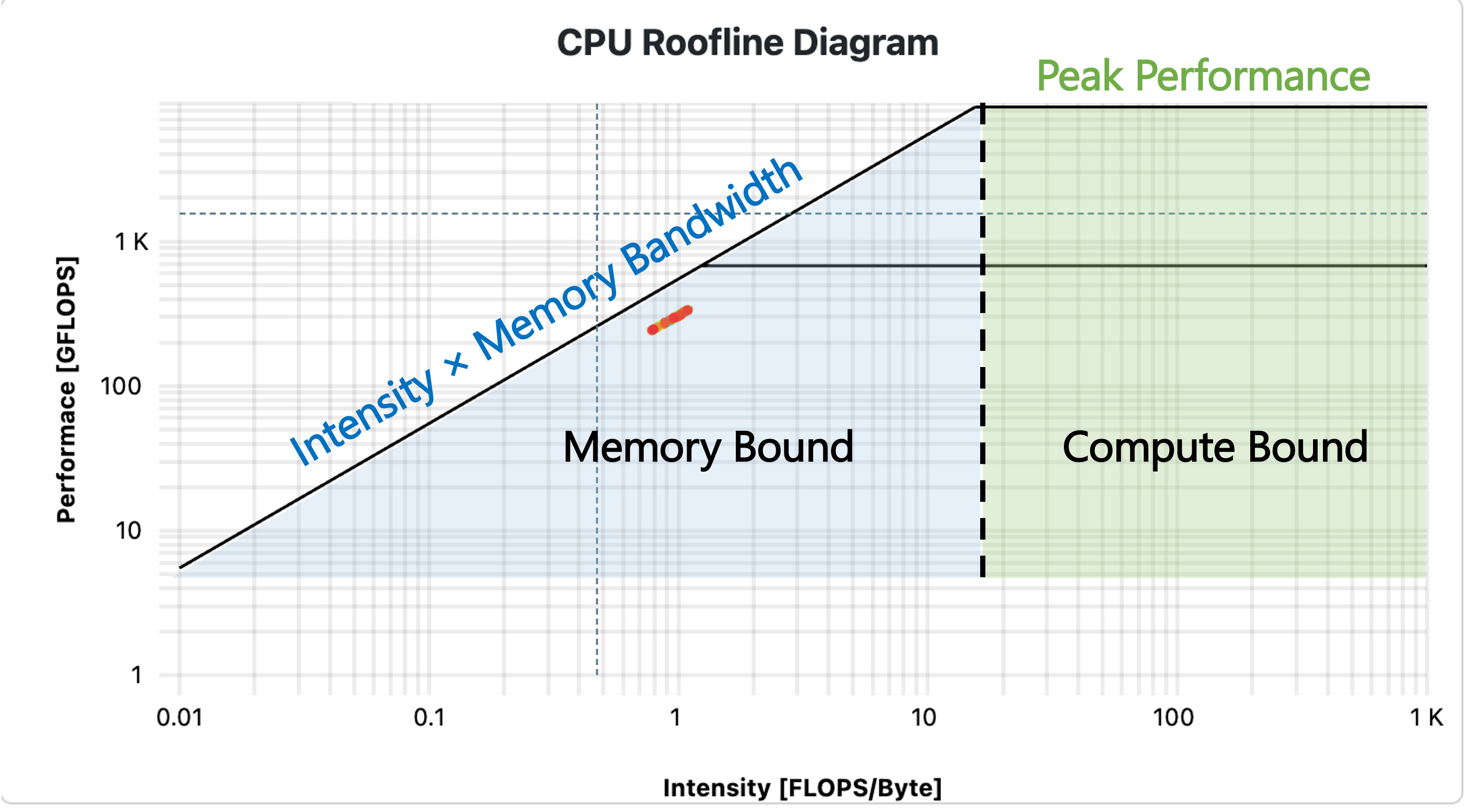
In jobs performing floating point operations on data read from memory, i.e. any numeric operation, which are very common in HPC, a Roofline plot is a common visualization of the jobs performance.

The x-axis is operational intensity: how many floating point operations are performed per byte loaded from memory. The y-axis is achieved performance: floating point operations per second.
A diagonal line marks the maximum performance possible. \[P_{peak} = \min(\text{Memory Bandwidth} \times \text{Operational Intensity},\ \text{Flop/s}_{peak})\]
A job with low intensity i.e. high memory transfers is pinned close to diagonal line: memory is the bottleneck, no matter how fast the CPU could otherwise compute.
The two horizontal lines mark the maximum performance possible if CPU computation itself is the limit: lower line for scalar operations, a higher one once vectorized instructions are used.
Where the diagonal and horizontal lines meet is the knee. Left of the knee = memory bound (data movement is the bottleneck). Right of the knee = compute bound (calculation capability is the bottleneck).
The colored dots show measurements taken at different points in time during the job’s run, following a blue-to-red gradient: blue marks the start of the application, red marks the end. Their position relative to the rooflines shows how close each phase of execution came to the physical performance limits, and how that changed over the runtime.

Discussion

Below is the Roofline plot for our application. 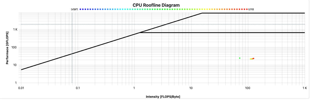Cluster Cockpit Roofline plot of a job

Take a moment to look at where our raytracer’s dot(s) land on the plot.

Is the job compute bound or memory bound? Which side of the knee do the measurements fall on?
Do the dots sit close to the scalar roofline, or closer to the vectorized roofline? What does that tell you about whether the application is actually using vectorized instructions?
Given where the job sits, which metric is more interesting for our next investigation — flops_any, or mem_bw? Which one, if improved, would actually move the dot closer to a roofline?
Does the dot’s position stay roughly constant over the blue-to-red timeline, or does it drift? What might cause a job to move further from (or closer to) the roofline as it runs?

CPU Metrics

CPU performance can be categorized in

Front-end utilization: preparation and scheduling of instructions of program code provided through the cache hierarchy
Computation: Arithmetic and logical operations with various data types, including the utilization of vectorized instructions, etc.
Back-end utilization: loading and storing of data in the cache hierarchy

The front- and backend hardware of a physical CPU core is often duplicated to implement simultaneous multithreading (SMT, also called hyperthreading). Here, the arithmetic logical unit receives data and instructions from two independent threads to achieve a sufficient amount, which is a common limiting factor in everyday calculations. On HPC systems, the benefit of SMT is very much application-dependent. It is often disabled on HPC systems, since code is optimized to maximize computational intensity.

ClusterCockpit captures many dedicated CPU metrics and provides a timeline visualization for each.

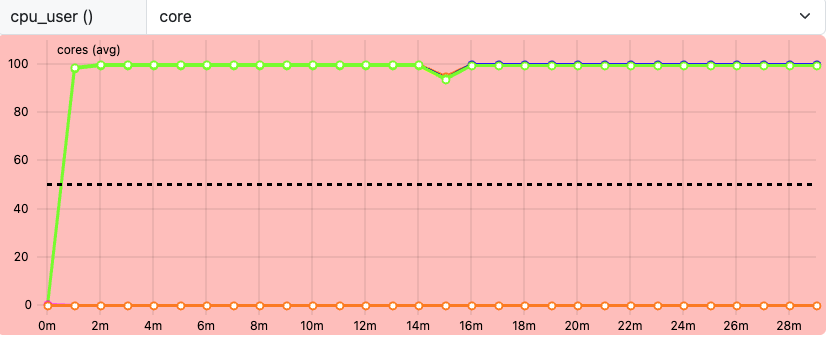
cpu_user shows, per core, the share of CPU time spent executing our application’s own instructions, as opposed to time spent in kernel/system activity or sitting idle. A high cpu_user near $1$ is a good sign: the core is busy, and busy doing our work rather than system overhead. A core sitting noticeably below $1$ is worth a closer look. Some of its time is going to something other than our application’s own instructions, whether that’s kernel activity, waiting, or other overhead. A cpu_user of $0$ means the core was idle for that interval and not running our application at all.

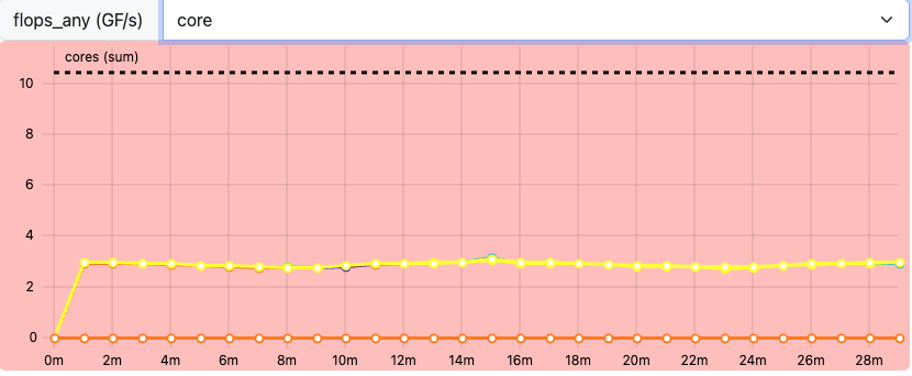
flops_any captures any floating point operation on Intel CPUs, at core-level granularity, with single- and double-precision operations accumulated into the same value. Recall from the Footprint panel that our job’s flops_any (avg) sat at only $22.38$ GF/s, while the node’s theoretical peak is $8532$ GF/s.

That gap looks enormous, but it isn’t a fair comparison yet: the $8532$ GF/s peak is for all $96$ cores of the exclusive node, while our job only ever uses $8$ of them. Scaled down to $8$ cores, the theoretical peak is roughly $711$ GF/s, so $22.38$ GF/s is still well below what our $8$ cores could theoretically achieve, but nowhere near the dramatic 96-core gap the raw numbers first suggest. This isn’t a contradiction of the Roofline plot classifying the job as compute bound either way: compute bound only means the CPU’s calculation capability is the limiting factor relative to how little data is moved, not that the job is issuing many floating point operations specifically.

Challenge

Exercise: Compare `flops_any` between job 1 and job 2

We now have two jobs to compare: our job1 (raytracer) and a job2 run with the raytracer_float4 executable.

Look at the flops_any metric for both jobs. What’s different between them, and why?

Show me the solution

ClusterCockpit flops_any metric for job2

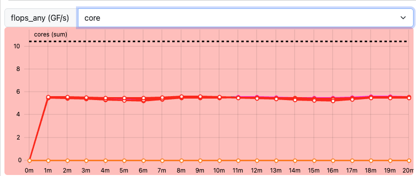
In our measurements, flops_any (avg) per core is close to $3$ GF/s for job 1, and close to $6$ GF/s for job 2, roughly a $2\times$ increase.

raytracer_float4 uses SIMD: float4 corresponds to SSE2 vectorized instructions, where a single instruction operates on $4$ float operands at once, instead of one operand at a time as in the original scalar raytracer.

flops_any counts floating point operations regardless of whether they were issued as scalar or vectorized instructions, each vectorized instruction in job 2 is counted as $4$ floating point operations rather than $1$. As a result, flops_any (avg) for job 2 is noticeably higher than for job 1. For the same amount of work done, the vectorized version issues far fewer instructions to do it, and each one accomplishes $4\times$ as much.

This is also a good moment to connect back to the Roofline plot: job 2’s dots sit slightly higher on the plot than job 1’s, and also shift further right along the x-axis — since computing more FLOPs per byte loaded raises the operational intensity too. They don’t touch the upper, vectorized roofline yet — that would become more visible if we used the full node instead of just $8$ of its $96$ cores.

Our raytracer performs plenty of integer, branching, and memory-addressing work per byte loaded, which does not count towards flops_any. This is why a low flops_any is not necessarily a red flag here. On top of that, our original raytracer is not vectorized. It issues one scalar floating point operation at a time rather than operating on multiple values per instruction, which further caps how high flops_any can climb regardless of how well the rest of the code performs.

Memory Metrics

Memory utilization is characterized in terms of used capacity, bandwidth and access latencies.

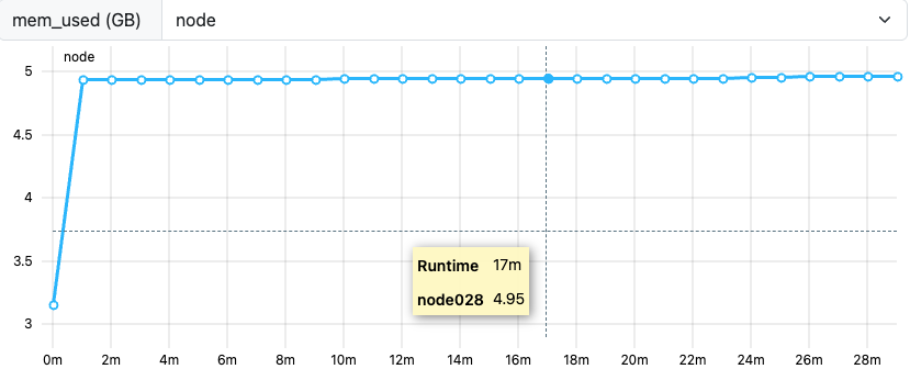
mem_used sits at approximately $5$ GB for our job, shown as an almost flat, straight line across the runtime, which is a good sign. A flat line means memory consumption is stable once the application has allocated what it needs. A slanted, steadily increasing line instead would be a warning sign of a memory leak: memory that is allocated but never freed, growing continuously over the job’s runtime instead of leveling off.

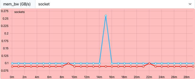
mem_bw is a socket-level metric. It measures how much memory is transferred to and from a given CPU socket per second, not per individual core. Since our node has multiple sockets, you’ll typically see a different mem_bw value reported for each socket. This difference depends entirely on which cores on each socket are actually active and running part of the application: a socket with more of our job’s cores running on it will show higher memory traffic than a socket with fewer (or none) of them active.

Energy

Depending on the ClusterCockpit configuration, an energy demand is displayed below the job info panels. This measurement is highly dependent on hardware configurations of your HPC systems, so the estimates may vary. They are often based on CPU package power measurements, which are unlikely to cover the whole energy demand of the node, e.g. omitting disks, fans, etc. In other cases, the energy may be estimated from power supply measurements and scaled to CPU activity to get a more accurate estimate.

These estimates often still not include network, parallel filesystem components and cooling of the clusters. Nevertheless, the estimate is a great tool to identify the scale of the jobs energy demand.

Miscellaneous

Typically, many more measurements and perspectives on the data are available for each tool.

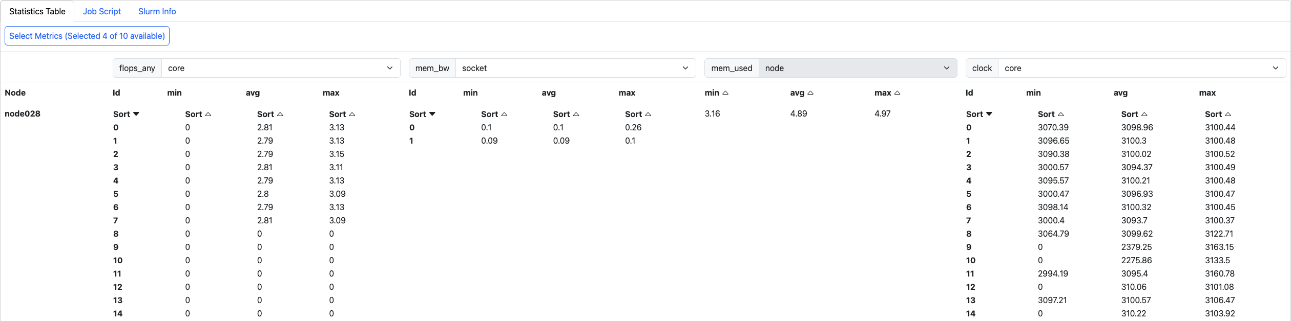
ClusterCockpit provides a detailed statistics table covering all measurements involved with a job. Alongside this table, you can also see your job script and Slurm info, which tells you how much of each resource was actually allocated to your job. The statistics table itself shows the max, min, and avg values for whichever metrics have been configured for your ClusterCockpit deployment.

How to identify a bottleneck?

Challenge

Exercise: Match application behavior to hardware

Which parts of the computer hardware may become a point of contention for these application patterns:

Calculating matrix multiplications
Reading data from processes on other computers
Calling many different functions from many equally likely if/else branches
Writing very large files (TB)
Comparing strings for matches
Constructing a large simulation model
Reading thousands of small files for each iteration

Maybe not the best questions, also missing something for accelerators.

Show me the solution

CPU (FLOPS), maybe the cache hierarchy if matrix elements do not align well to cache sizes
I/O (network)
CPU (Front-End), difficult to prepare instructions in time
I/O (disk), bandwidth limited
CPU (Back-End), getting strings through the caches
Memory (capacity)
I/O (disk)

Summary

Dedicated performance measurement tools are helpful to create reports of the general job behavior. These tools either trace every event, or sample the application and hardware state at regular intervals. Many tools are available, but some may have to be set up by the HPC system administrators, or rely on valid licenses.

The relationship between a job and the execution on physical hardware can become a very deep topic. One of these topics is the correct mapping of job processes to the requested number of CPU cores, addressed in the next episode.

Key Points

Performance tools measure data as regular samples or by tracing every event
The data is either processed and visualized in a timeline or aggregated in a final profile
Job performance relates closely to contention points in physical hardware
- CPU utilization (front-end, ALU, back-end), multithreading, vectorization
- Memory utilization (capacity, bandwidth, latency)
- Disk I/O
- Network I/O

Content from Pinning

Last updated on 2026-08-13 | Edit this page

Overview

Questions

What is “pinning” of job resources?
How can pinning improve the performance?
How can I see, if pinning resources would help?
What requirement hints can I give to the scheduler?

Objectives

After completing this episode, participants should be able to …

Define the concept of “pinning” and how it can affect job performance.
Name Slurms options for memory- and cpu- binding.
Use hints to tell Slurm how to optimize their job allocation.

The benchmark code used in this episode

Let us first prepare a so-called benchmark for doing some pinning experiments in this episode. In a HPC context, a benchmark is a software that implements and runs CPU- and memory-intensive computations in a well-measurable way. Many different benchmarks exist. Here, we employ the STREAM benchmark, because it is deliberately designed to mimic computations that are memory-bandwidth limited.

The STREAM benchmark may already be available on your system. Check the module environment. If not, it can be installed with:

BASH

# download, it is only a single C-program
wget https://www.cs.virginia.edu/stream/FTP/Code/stream.c
# compile, may need appropriate module to make gcc available, enable OpenMP
gcc -O3 -fopenmp -DSTREAM_ARRAY_SIZE=100000000 -DNTIMES=20 stream.c -o stream

This creates the executable stream.

Running `stream`

To get aquainted with the output of stream, run it:

BASH

./stream

An sample output is:

OUTPUT

-------------------------------------------------------------
STREAM version $Revision: 5.10 $
-------------------------------------------------------------
This system uses 8 bytes per array element.
-------------------------------------------------------------
Array size = 100000000 (elements), Offset = 0 (elements)
Memory per array = 762.9 MiB (= 0.7 GiB).
Total memory required = 2288.8 MiB (= 2.2 GiB).
Each kernel will be executed 20 times.
 The *best* time for each kernel (excluding the first iteration)
 will be used to compute the reported bandwidth.
-------------------------------------------------------------
Number of Threads requested = 192
Number of Threads counted = 192
-------------------------------------------------------------
Your clock granularity/precision appears to be 1 microseconds.
Each test below will take on the order of 12271 microseconds.
   (= 12271 clock ticks)
Increase the size of the arrays if this shows that
you are not getting at least 20 clock ticks per test.
-------------------------------------------------------------
WARNING -- The above is only a rough guideline.
For best results, please be sure you know the
precision of your system timer.
-------------------------------------------------------------
Function    Best Rate MB/s  Avg time     Min time     Max time
Copy:          179291.6     0.014355     0.008924     0.019452
Scale:         184755.8     0.013567     0.008660     0.015317
Add:           175990.9     0.015244     0.013637     0.016602
Triad:         172339.1     0.015706     0.013926     0.020396
-------------------------------------------------------------
Solution Validates: avg error less than 1.000000e-13 on all three arrays
-------------------------------------------------------------

Understanding the output

The benchmark reports the achieved memory bandwidth for four simple operations:

Copy:   a[i] = b[i]
Scale:  a[i] = q * b[i]
Add:    a[i] = b[i] + c[i]
Triad:  a[i] = b[i] + q * c[i]

These are operations that make up the main work in numerical codes when they loop over large arrays. Improving code efficiency involves minimizing the overhead associated with accessing the memory of such large arrays during computations. This is where pinning (or binding) will come into play later in this episode. The reported Best Rate (MB/s) is the highest sustained memory bandwidth achieved for each operation.

The first notable metric is the “Number of Threads” (requested and counted, here 192). This should appear given that stream was compiled with OpenMP (-fopenmp). We will treat threads in more detail soon. The other output of interest is the bandwidth in MB/s reported at the bottom for the four types of array operations, copy, scale, add and triad. The higher the bandwidth, the faster these array operations can complete.

Setting up the HPC kitchen: CPUs, processes, threads, tasks

We first want to agree on some terminology. This is motivated by the fact that in HPC the same words can mean slightly different things depending on whether you are talking about the operating system, the scheduler (Slurm), or in the context of a parallel programming model (MPI or OpenMP). While this episode is called “Pinning”, you will notice that many pinning-related command options contain the string “bind”, also in Slurm. Hence, we will also use the synonym “Binding” in the following.

What is a CPU in a pinning/binding context?

Let us clarify some potential confusion around the word “CPU”, as it is somewhat overloaded. Hardware vendors often use “CPU” to mean the whole processor chip. That chip contains multiple independent execution units:

A core is the physical execution unit on the chip — the actual hardware that runs instructions.
A thread is the logical execution unit exposed by a core. If simultaneous multithreading (SMT) is off, one core provides exactly one thread, so the two are the same thing. If SMT is on, one physical core provides two (or more) threads, each independently schedulable.

This physical-vs-logical distinction matters because the number of logical execution units (threads) can be larger than the number of physical cores actually present.

In Linux and Slurm, CPU refers to a thread - logical execution unit - not the physical processor chip. And:

We will use quite a few Slurm commands below. Slurm command options often contain “cpu”, for example --cpus-per-task. This is because a CPU in Slurm is: 1 logical execution unit = 1 Slurm-CPU.
A Slurm-CPU is a schedulable execution unit visible to the operating system.
In general: 1 Slurm-CPU = 1 physical CPU core, but not always, sometimes with SMT enabled: 2 or more Slurm-CPUs constitute 1 physical CPU core.
The Slurm option --cpus-per-task determines how many threads Slurm allocates.

Show details

Historically, CPU refers to the physical processor chip. For example, a compute node might have two CPU sockets (two processor chips). If each socket hosts 32 physical cores, we have:

2 physical CPUs (sockets) = 2 x 32 cores = 64 cores = 64 Slurm-CPUs

However, the physical CPU hardware can pretend to have more cores than physically present. This is called Simultaneous Multithreading (SMT), or Hyperthreading for Intel processors. Then,

2 physical CPUs (sockets) = 2 x 32 cores x 2 SMT threads = 128 logical CPUs = 128 Slurm-CPUs

Therefore, on systems without SMT, a Slurm CPU corresponds to a physical core. On systems with SMT enabled, multiple logical execution units map onto a physical core. People then also talk about hardware threads, A hardware thread is a feature of the processor that allows a core to execute more than one software thread at a time. With SMT,
1 Slurm CPU = 1 hardware thread, and
2 Slurm CPUs = 2 hardware threads = 1 physical core.
Be aware that “thread” is another expression being a bit overused. From now on, we will refer to thread as something only on the software layer. This will be explained below.

Processes

Time to run our stream program in an “HPC-way”. We are now on a HPC compute node. You may be on the login node, the landing point when you ssh-ed from your own machine. In case, you cannot run jobs on the login node, you will need to allocate some resources first:

BASH

salloc --ntasks=2 --cpus-per-task=24 --nodes=1 --mem=5G

Now we use Slurm’s tool srun for running parallel jobs. Launch the following two runs:

BASH

# if you did not do the `salloc`: add the option `--mem=4G` after each `srun`.
srun --ntasks=1 ./stream
srun --ntasks=2 ./stream

In the first run, the operating system creates one process which will be associated with stream. This process is an isolated entity as it does not directly share the following things with other processes:

virtual memory,
process ID (PID),
file descriptors.

Think of a process resembling a large kitchen. This kitchen has its own ingredients, utensils, recipes and storage space. Other kitchens do not have direct access to it.

When running the second job with --ntasks=2, Slurm commissioned two such kitchens. Again, they work independently. Therefore you see the stream output twice.

Challenge

Multiple tasks

When running srun --ntasks=2 ./stream, you may have noticed differing outputs for the two bandwidth summaries (copy, scale, add ,triad). Why are these not identical?

Give me a hint

As in the kitchen analogy, the two tasks (kitchens) run independently, that is, they do not even know about each other.

Show me the solution

The two stream tasks denote two independent processes that may also occupy different (Slurm-)CPU resources. Hence, with multiple CPUs, their runtimes and bandwidth outcomes will never be exactly identical.

Tasks

In the above srun commands, Slurm uses the options --ntasks, and not something like --nprocesses. A task is Slurm’s term for an independent unit of work that the scheduler starts, places on resources and manages. In most cases: 1 task = 1 process.

Back to the kitchen analogy. Imagine the stream computing job would be a catering order. Then, Slurm would be the event manager. It manages the resources you requested, which may be one (--ntasks=1) or two (--ntasks=2) kitchens.

Show details

Slurm uses the term “task” because it is a scheduler concept rather than an operating-system concept. While in most HPC applications, one task corresponds to one process, Slurm is more general by treating a task as something overarching a process, some kind of workload to be scheduled onto (Slurm-)CPUs. In other words, the Slurm scheduler doesn’t manage kitchens directly. Instead, it acts as the event manager making sure the workload runs on the available resources requested via --ntasks, and other options.

Now, what about the cooks working in a kitchen? One kitchen can employ one or multiple cooks, in other words, a process can have one or more threads.

Threads

Threads live inside a process and

share the same memory (kitchen storage space),
can access the same variables (ingredients and utensils),
execute concurrently (multiple cooks working simultaneously).

A thread is also referred to as an execution stream within a process that shares memory with other threads in the same process. So the threads are like the cooks being busy in the same kitchen. They can

share the ingredients,
share the utensils,
can cooperate.

Threads may sometimes get in each other’s way, unless they are told not to move around the kitchen by “pinning” them to their work area. We will get to that.

So let’s assign four CPUs to one task:

BASH

srun --ntasks=1 --cpus-per-task=4 ./stream

where now the output for “Number of Threads” will most likely show the number 4. The stream runtime is programmed such that it detects four available CPUs and therefore creates four threads by default.

Multiple cooks: OpenMP

In case you want to try again, put time in front of every srun and check the parallel against the sum of the sequential runtimes.

The stream program is an OpenMP-parallel program. The large loops of array operations are distributed over OpenMP-threads. The thread number can be set via the environment variable OMP_NUM_THREADS:

BASH

export OMP_NUM_THREADS=4
srun --ntasks=1 ./stream

Show details

The Slurm option --cpus-per-task determines how many CPUs Slurm allocates, while OMP_NUM_THREADS determines how many OpenMP threads the application creates. Slurm does not automatically force OpenMP to obey --cpus-per-task. Therefore, users should normally set

BASH

export OMP_NUM_THREADS=$SLURM_CPUS_PER_TASK

after setting CPUs/task via Slurm directives. This sets number of OpenMP threads = number of CPUs. Otherwise, ending up with number of OpenMP threads > number of CPUs would involve an oversubscription of the allocated CPUs.

Challenge

Understanding `OMP_NUM_THREADS`

When you do

BASH

export OMP_NUM_THREADS=4
srun --ntasks=1 --cpus-per-task=3 ./stream

what is the actual count stream reports under “Number of Threads”.

Give me a hint

Remember that stream is an OpenMP-parallel program.

Show me the solution

The count is likely reported as Number of Threads counted = 4. Since stream is an OpenMP-parallel program, setting OMP_NUM_THREADS=4 will be evaluated inside the program. However, Slurm only allocated 3 CPUs via --cpus-per-task=3, which is fine but will oversubscribe the CPU resources.

Challenge

Understanding `OMP_NUM_THREADS` more

In case you did the previous challenge, now run this:

BASH

srun --ntasks=1 --cpus-per-task=3 ./stream

What is the actual count reported under “Number of Threads”?

Give me a hint

In the previous challenge you set OMP_NUM_THREADS. What happened to it?

Show me the solution

Your earlier setting export OMP_NUM_THREADS=4 is still active, unless you have changed the terminal. Hence, the count is still reported as Number of Threads counted = 4. If you do

BASH

unset OMP_NUM_THREADS
srun --ntasks=1 --cpus-per-task=3 ./stream

this will indeed produce Number of Threads counted = 3.

Multiple kitchens: MPI

Before, we assigned multiple threads to one process, that is, we put four cooks into one kitchen. Now suppose, the catering job is so large that one 4-cook kitchen is not enough. This leads to the MPI programming model. Assume the workload requires running two independent kitchens. In fact, we have already done this:

BASH

unset OMP_NUM_THREADS # reset in order to undo earlier settings
srun --ntasks=2 ./stream

where each task is a separate MPI process. MPI-parallel programs involve data exchange between processes (or Slurm tasks). Note that stream it is not programmed to have this feature. However, like every program, it can be run as multiple independent process instances.

Multiple cooks + kitchens: OpenMP + MPI

Parallel programs can also combine the OpenMP and MPI models, sometimes referred to as a hybrid model. So let’s now run such a hybrid “2-kitchens, 4-cooks-per-kitchen” job:

BASH

srun --ntasks=2 --cpus-per-task=4 ./stream

This will involve a total of 8 CPUs.

Challenge

Requesting resources for a hybrid parallel program

You want to request resources for a hybrid OpenMP - MPI parallel program. The estimated workload consists of two processes where each process itself involves three threads. What are the two options submitting an srun command for this?

Give me a hint

Remember that a process is almost always equivalent to a Slurm task. Also, OpenMP uses the environment variable OMP_NUM_THREADS to set the thread count.

Show me the solution

BASH

# Option 1)
srun --ntasks=2 --cpus-per-task=3 ./stream
# Option 2)
export OMP_NUM_THREADS=3
srun --ntasks=2 ./stream

Managing the kitchen: The Linux scheduler

By now, we have gained some decent understanding about tasks and threads and how they make up a parallel run. So we are almost ready to see how to control CPU alignment in parallel runs via pinning. There is one more thing useful to know about.

In our kitchen analogy, we referred to Slurm as the event manager, who takes care of the whole catering job without getting involved with the cooks (CPUs) inside the kitchen(s). However, on the lower kitchen level, there is actually another manager. This is the Linux scheduler. Similar to rotating cooks around the kitchen’s different workstations, where a workstation equates a (Slurm-)CPU, the Linux scheduler may migrate threads between CPUs during execution.

Thread migration happens by default because Linux is designed to optimize overall system responsiveness and throughput, not necessarily the performance of a single process.

Show details

How can we observe thread migration? Let’s first create another version of our benchmark. This is a version that will run a bit longer:

BASH

gcc -O3 -fopenmp -DSTREAM_ARRAY_SIZE=100000000 -DNTIMES=100 stream.c -o stream_long

Now open a second terminal on the same compute node where you have been running stream and type

BASH

srun --pty --overlap --jobid=<id> /bin/bash
watch -n 0.5 'ps -eLo pid,tid,psr,comm | grep stream_long

The watch command keeps an eye on repeated calls to ps which then greps for running stream processes. Back in the original terminal, employ 12 CPUs by running the new version, stream_long:

BASH

srun --pty --overlap --jobid=<id> /bin/bash
export OMP_NUM_THREADS=12
./stream_long

Now, observe the 12 processes showing up in the second terminal. The numbers in the third column are likely to change occasionally. The manpage of ps refers to that number as the “processor that process is currently assigned to”, which in our context is the CPU number. Threads are being moved around when it changes.

To optimize a selected process entails removing the overhead due to its moving threads. This requires extra directives to keep the cooks at their workstations, so they don’t bump into each other, that is, to pin or bind them.

Binding 1: CPU affinity

Pinning, or binding, is the assignment of processes or threads to specific CPU resources so that the operating system does not freely move them between CPUs. This is also called CPU affinity. In the run

BASH

unset OMP_NUM_THREADS # reset in order to undo earlier settings
srun --ntasks=1 --cpus-per-task=3 --cpu-bind=cores ./stream

the option --cpu-bind=cores binds a task and its threads to the Slurm CPUs allocated to it. On systems without SMT/Hyperthreading, these CPUs correspond to physical cores. For example, suppose the above run allocated CPUs 48-50. Then Slurm will create an affinity mask like: Allowed CPUs = {48,49,50} for that task.

Challenge

Displaying information about the CPU architecture: `lscpu`

The command lscpu gathers CPU architecture information. Give it a try and see how many CPUs are reported. The end of the output will show something about “NUMA”. Can you figure out the number of NUMA nodes on your system? Any idea what this is?

Give me a hint

lscpu will first report the CPU architecture, then number of CPUs. You will see that CPUs are grouped into “NUMA nodes”.

Show me the solution

An example output of lscpu is as follows (some output truncated):

OUTPUT

Architecture:                x86_64
  CPU op-mode(s):            32-bit, 64-bit
  Address sizes:             46 bits physical, 57 bits virtual
  Byte Order:                Little Endian
CPU(s):                      192
  On-line CPU(s) list:       0-191
Vendor ID:                   AuthenticAMD
  Model name:                AMD EPYC 9654 96-Core Processor
    CPU family:              25
    Model:                   17
    Thread(s) per core:      1
    Core(s) per socket:      96
    Socket(s):               2
[ ... text truncated ... ]
NUMA:
  NUMA node(s):              8
  NUMA node0 CPU(s):         0-23
  NUMA node1 CPU(s):         24-47
[ ... text truncated ... ]
  NUMA node7 CPU(s):         168-191

Here, the CPU architecture consists of two sockets with 96 physical cores per socket, totaling 192 CPUs. We further see 8 NUMA nodes, each listing CPU ranges. NUMA nodes appear to be some regions dividing the CPUs into groups with 24 consecutive CPU numbers. So these NUMA regions seem to resemble something like “areas of jurisdiction” over the CPU entirety.

Non-Uniform Memory Access (NUMA)

Non-Uniform Memory Access (NUMA) is a computer memory design used in multiprocessor systems. Memory access time depends on where the memory is located relative to the accessing processor. In a NUMA system, the architecture is divided into multiple regions called NUMA nodes. A single compute node can contain several NUMA nodes. Each NUMA node contains one or more cores along with the portion of the system’s memory that is local to it - meaning that CPU can access it faster than memory attached to a different NUMA node. Memory isn’t exclusive to a NUMA node, though: a core can still access another NUMA node’s memory, just at higher latency and/or lower bandwidth, which is precisely what makes access “non-uniform” rather than a fixed cost regardless of location.

Your personal laptop may have only one node, while a HPC system is likely to have more.

Binding 2: Memory affinity

On NUMA systems, memory attached to nearby CPUs can be accessed faster than memory from distant CPUs. Moreoever, when a thread repeatedly runs on the same CPU, data already stored in the CPU’s cache can be reused. On the other hand, if the operating system moves the thread to another CPU, some of that advantage due to data locality may be lost. Therefore, CPU affinity goes hand in hand with memory affinity to keep computation and data close together. The run

BASH

srun --ntasks=1 --cpus-per-task=3 --mem-bind=local ./stream

tries to allocate memory close to the CPUs running the task, that is, within the NUMA node of those CPUs. In such a context, people also talk about minimizing memory access latency.

Show details

Latency in computing refers to the time delay between the initiation of an action and the resulting output or response. Therefore, it represents a “wait time”, rather than the speed of a data transfer (bandwidth). Latency is measured in milliseconds or microseconds, while bandwidth is measured in bits per second.

Performance metric	Meaning	Measured in
latency	wait time	ms, $\mu$s
bandwidth	maximum rate of data transer	bps, Mbps, Gbps

Before pinning, understand Slurm’s configuration

The CPU/memory-binding behaviour is not the same across different HPC systems. For example, the srun documentation cautions that the --mem-bind option is “used only when the task/affinity plugin is enabled and the NUMA memory functions are available.” Further it says, “Note that the resolution of CPU and memory binding may differ on some architectures.” It is thus recommended to determine the specific configuration of your system via a self-reporting run:

BASH

srun --ntasks=2 --cpus-per-task=4 --cpu-bind=verbose,none --mem-bind=verbose,none ./stream

where Slurm’s output (omitting the stream output) may be:

OUTPUT

cpu-bind=MASK - computenode14032, task  0  0 [447219]: mask 0x3fffc0000000000 set
cpu-bind=MASK - computenode14032, task  1  1 [447220]: mask 0x3fffc0000000000 set
mem-bind=NONE - computenode14032, task  0  0 [447219]: mask 0xff
mem-bind=NONE - computenode14032, task  1  1 [447220]: mask 0xff

In this output, the first two lines correspond to the CPU masks. The mask essentially shows which CPUs a task is allowed to use. No need to decrypt the hexadecimal output after “mask” for now. The fact that these masks are identical for both tasks, here 0x3fffc0000000000, indicates that both tasks were allowed to run on the same set of CPUs.

The memory binding information in the last two lines shows which NUMA nodes are available for memory allocation. Here, the output mem-bind=NONE shows that memory allocation was unrestricted across all NUMA nodes.

Now try with CPU-binding enabled:

BASH

srun --ntasks=2 --cpus-per-task=4 --cpu-bind=verbose,cores ./stream

telling Slurm to try to give each task its own set of cores. Most likely, you will then see different mask codes, like in our example:

OUTPUT

cpu-bind=MASK - computenode14032, task  0  0 [460428]: mask 0x3c0000000000 set
cpu-bind=MASK - computenode14032, task  1  1 [460429]: mask 0x3c00000000000 set

which is what we wanted.

Finally, let’s make this cryptical mask output human-readable:

BASH

srun --ntasks=2 --cpus-per-task=8 --cpu-bind=verbose,cores \
     bash -c 'grep Cpus_allowed_list /proc/self/status'

Voilà

OUTPUT

cpu-bind=MASK - computenode14032, task  0  0 [459142]: mask 0x3fc0000000000 set
cpu-bind=MASK - computenode14032, task  1  1 [459143]: mask 0x3fc000000000000 set
Cpus_allowed_list:	42-49
Cpus_allowed_list:	50-57

Now we can see how the different masks correspond to non-overlapping CPU sets.

Probing Slurm’s default behaviour will help understand what to expect when enforcing CPU/memory binding.

Giving Slurm a hint

You can advise Slurm to bind tasks according to application hints. Let’s look at two hint types that are closely related to CPU- and memory-binding:

BASH

srun --ntasks=1 --cpus-per-task=4 --hint=compute_bound ./stream

The option --hint=compute_bound tells Slurm that the application is expected to spend most of its time performing computations.

BASH

srun --ntasks=1 --cpus-per-task=4 --hint=memory_bound ./stream

The option --hint=memory_bound tells Slurm that the application is expected to spend much of its time moving data between memory and CPUs.

Again, the exact behavior of --hint will be site-dependent. Some clusters may ignore certain hints, while others use them to influence CPU placement and affinity settings.

Moreover, while hints provide guidance to the scheduler, they do not guarantee a particular placement. On some systems, the default placement may already be well suited to the application, resulting in no observable performance difference.

Investigate your system by cross-comparing the above two runs against a third one without hints:

BASH

srun --ntasks=1 --cpus-per-task=4 ./stream

Show details

On most HPC systems, the default Slurm configuration already keeps tasks reasonably close to their memory. Therefore, there may be only little performance difference between the default execution and runs that use CPU/memory binding explicitly or via hints.

Controlling NUMA: `numactl`

NUMA nodes are interconnected, allowing CPUs to access both their own memory and that from other nodes. The tool numactl can alter the default memory-access behavior of the Linux scheduler. This can be useful for studying the potential benefit of binding before launching production runs.

You can get an overview over the NUMA nodes of the machine where you run:

BASH

numactl --hardware

This shows the whole node inventory, adding some details to the earlier lscpu output. On an 8-node architecture, it could look like this:

OUTPUT

available: 8 nodes (0-7)
node 0 cpus: 0 1 2 3 4 5 6 7 8 9 10 11 12 13 14 15 16 17 18 19 20 21 22 23
node 0 size: 192453 MB
node 0 free: 176208 MB
node 1 cpus: 24 25 26 27 28 29 30 31 32 33 34 35 36 37 38 39 40 41 42 43 44 45 46 47
node 1 size: 193529 MB
node 1 free: 186718 MB
[ ... text truncated ... ]
node 7 cpus: 168 169 170 171 172 173 174 175 176 177 178 179 180 181 182 183 184 185 186 187 188 189 190 191
node 7 size: 193421 MB
node 7 free: 173933 MB
node distances:
node     0    1    2    3    4    5    6    7
   0:   10   12   12   12   32   32   32   32
   1:   12   10   12   12   32   32   32   32
   2:   12   12   10   12   32   32   32   32
   3:   12   12   12   10   32   32   32   32
   4:   32   32   32   32   10   12   12   12
   5:   32   32   32   32   12   10   12   12
   6:   32   32   32   32   12   12   10   12
   7:   32   32   32   32   12   12   12   10

One can see the assignment of the total of 192 CPUs to 8 nodes, in addition to each node’s memory available. The trailing output “node distances” shows a matrix with memory access latency between node pairs.

Show details

When you run numactl --hardware, the node distance matrix lets you select two nodes given by a row-column pair, and find the associated node distance. Node distance is related to the memory access latency when CPUs of different nodes exchange data. Staying on the same node has the lowest latency (10 in the above example), which you find on the diagonal of the matrix. Further, the matrix is symmetric, indicating that on node A, fetching data from node B has the same latency as the reverse way.

Investigating binding via `numactl`

Before executing production runs, it may be useful to investigate potential latencies on your NUMA system. The tool numactl allows for a more fine-grained control because one can deliberately place computation and memory on different NUMA nodes.

So let’s put stream to work once more. Placing both CPU and memory on node 0 is done as follows:

BASH

numactl --cpunodebind=0 --membind=0 ./stream

The two options --cpunodebind and --membind are to some degree the counterparts of the srun options --cpu-bind and --mem-bind. To be more accurate:

--cpunodebind restricts execution to CPUs belonging to a NUMA node.
--membind allocates memory from a specific NUMA node.

Compare the above run with one where we put the CPUs on a different node:

BASH

numactl --cpunodebind=N --membind=0 ./stream

By setting N>0, CPUs are placed on nodes away from 0, while memory stays on 0. Can you see a correlation between increasing N and bandwidth?

Challenge

Observing thread count on NUMA nodes

First and foremost unset OMP_NUM_THREADS
Compare the output for “Number of Threads” between the run numactl ./stream and a corresponding run with CPU-binding to node 0. You may see a different “Number of Threads”. If that is the case, which one is smaller and why?

Give me a hint

CPU-binding to node 0 is done using the option --cpunodebind=0.

Show me the solution

CPU-binding to node 0, without worrying about memory-binding, is done via

BASH

numactl --cpunodebind=0 ./stream

Generally, the thread count is the number of (logical) CPUs available to the process.

First run, without binding, numactl ./stream: This will involve all CPUs available to the process, which may encompass multiple nodes.
Second run, with binding, numactl --cpunodebind=0 ./stream: This will restrict to the CPUs of node 0.

In most cases, when your system has multiple (NUMA) nodes, the binding call will report a smaller count because fewer CPUs are accessible.

Challenge

Test different memory placement

Figure out the NUMA node number N which is farthest away from node 0 and perform two numactl runs with different memory placement. Let each run use 4 threads. Also, measure the runtime of the two runs. What do you observe in terms of performance and how would you explain differences?

Give me a hint

The most distant node N probably corresponds to the maximum node number. Either lscpu or numactl --hardware report node numbers.

Show me the solution

Assuming that N=7, launch one run on node 0 and the second on node 7.

BASH

export OMP_NUM_THREADS=4
time numactl --cpunodebind=0 --membind=0 ./stream
time numactl --cpunodebind=7 --membind=0 ./stream

The most likely outcome is that the second run will exhibit a smaller bandwidth as well as a longer runtime. The reason is memory access lateny, which increaes when computation and data storage happen on different nodes.

We have gained some overview over Slurm’s binding options as well as the kinds of lateny studies that can be performed using numactl. Note that many more parameters exist for controlling binding behaviour. The optimal parameter set depends on your application and the employed HPC system.

Key Points

A Slurm-CPU is a schedulable execution unit visible to the operating system.
A process usually equates a Slurm task and involves $\ge 1$ (Slurm-)CPUs.
OpenMP threads are software threads created by an application.
- It is common to run one OpenMP-thread per CPU.
Pinning, or binding, is to keep computation and data close together in order to improve performance through minimized latencies.
- The CPU- and memory-binding options of srun control resource allocation and placement of Slurm jobs.
- srun --cpu-bind ... controls where Slurm runs tasks, i.e., where computation runs.
- srun --mem-bind ... controls where Slurm allocates memory, i.e., where data is allocated.
The benefit of CPU and memory placement strongly depends on the application, cluster configuration and hardware.
On NUMA systems, CPU- and memory often go together to keep computation and data close to one another.
Hints provide guidance to Slurm about the expected characteristics of an application.
- srun --hint=compute_bound ... may be beneficial for applications that require many CPU resources.
- srun --hint=memory_bound ... may be beneficial for applications that are limited by memory bandwidth.
Memory-intensive applications are often more sensitive to NUMA locality than compute-intensive applications. The stream program is such a case.
numactl provides fine-grained control over CPU and memory placement.

Content from Performance of Accelerators

Last updated on 2026-08-13 | Edit this page

Overview

Questions

What are accelerators?
How do they affect my jobs performance?
How can I measure accelerator utilization?

Objectives

After completing this episode, participants should be able to …

Understand difference of performance measurements on accelerators (GPUs, FPGAs) to CPUs.
Understand how batch systems and performance measurements tools treat accelerators.

Introduction

Run the same example workload on GPU and compare.

Summary

Leading question: Performance optimization is a deep topic and we are not done learning. How could I continue exploring the topic?

Key Points

Tools to measure GPU/FPGA performance of a job
Common symptoms of GPU/FPGA problems

Content from Next Steps

Last updated on 2026-08-13 | Edit this page

Overview

Questions

What are other patterns of performance bottlenecks?
How to evaluate an application in more detail?

Objectives

After completing this episode, participants should be able to …

Find collection of performance patterns on hpc-wiki.info
Identify next steps to take with regard to performance optimization.

To be precise: Numerical efficiency

This has been moved from Introduction as it seems to be an abrupt transistion into Numerical efficiency.

Computational inefficiency is not limited to unnecessarily slow implementations. It can also arise when calculations are performed with a higher numerical precision than required for the scientific objective.

In scientific computing, numerical precision determines how accurately numbers are represented and processed by the CPU, for example through single-precision or double-precision floating-point arithmetic.

Higher numerical precision generally increases computational cost, memory usage, and data movement. Lower precision, on the other hand, can improve performance and reduce memory consumption, but may also reduce numerical accuracy and stability.

Choosing an appropriate numerical precision is therefore an important aspect of computational efficiency and depends strongly on the requirements of a given application.

Challenge

Compare numerical results

Our sum.bash implementation also demonstrates how numerical methods and implementation details can affect computational accuracy.

When running the two summation methods from the previous challenge, compare the final numerical results. Which result appears more accurate, and why? Is the inaccurate result smaller or larger than the expected value?

Give me a hint

Think again about the airplane analogy. Which scenario is more prone to small losses accumulating over time? 1. Passengers repeatedly handle their own individual baggage items. 2. Baggage is handled collectively in a single coordinated operation.

Show me the solution

The external loop implementation sum.bash and the internal bc one-liner may produce results similar to

OUTPUT

333833499.99999999999667056674 # bc, external loop (sum.bash)
333833500                      # bc, internal loop (one-liner)

where the exact floating-point representation may vary slightly between systems. The implementation in sum.bash repeatedly evaluates expressions involving logarithms and exponentials:

BASH

e(2 * l($i))

These operations introduce small numerical rounding errors during every loop iteration. Since the result is accumulated repeatedly, the rounding errors also accumulate over time. The one-liner implementation instead computes the powers directly inside a single bc execution context and therefore avoids much of the repeated conversion and evaluation overhead.

As a result, the value produced by sum.bash is typically slightly smaller than the mathematically expected result due to accumulated truncation and rounding effects. Although bc supports arbitrary precision arithmetic, the effective numerical precision still depends on how calculations are performed and how intermediate results are represented.

Next Steps

hpc-wiki.info - I/O - CPU Front End - CPU Back End - Memory leak - Oversubscription - Underutilization

Summary

Key Points

There are many profilers, some are language-specific, others are vendor-related, …
Simple profile with exclusive resources
Repeated measurements for reliability

All in One View

Overview

Questions

Objectives

Background

Measuring sleep with time

BASH

BASH

OUTPUT

Why does time sometimes produce different output?

BASH

BASH

BASH

BASH

BASH

Benchmarking and profiling

BASH

BASH

BASH

OUTPUT

BASH

OUTPUT

Time for a date

BASH

OUTPUT

Epoch time

BASH

OUTPUT

Building a stopwatch with date

BASH

Give me a hint

BASH

Show me the solution

BASH

Part 1: An inefficient job example

BASH

BASH

BASH

Identify the inefficient pieces

Give me a hint

Show me the solution

Let’s pull out our stopwatches

Give me a hint

Show me the solution

BASH

BASH

BASH

BASH

Speeding things up

BASH

Evaluate the runtime improvement

Give me a hint

Show me the solution

BASH

CPU-bound versus memory-bound

Part 2: About HPC power consumption

The more the merrier: Parallel resources

Measuring parallel runtime: core-hours

Other HPC resource types

A typical HPC computing job

How many core-hours does this job involve?

Give me a hint

Show me the solution

What are watt-hours?

Power-consuming hardware pieces

So what’s next?

Submit your first raytracer job with Slurm

BASH

Give me a hint

Show me the solution

OUTPUT

Overview

Questions

Objectives

Getting a feel for the size of your cluster

BASH

OUTPUT

Available partitions depend on the HPC system

Show me the solution

BASH

Measuring `sleep` with `time`

Time for a `date`

Building a stopwatch with `date`

How much `--mem` do I get?

The `seff` tool

`seff` may not be available

The `sacct` tool