Welcome to this workshop
Overview
Teaching: 10 min
Exercises: 0 minQuestions
What is the purpose of this training?
What are the learning goals and objectives?
What will this workshop not cover?
What next steps should be taken after this course?
Objectives
Contextualising Data Science, AI and ML for Biomedical Researchers
Understanding the scope and coverage of the topics within this workshop
Getting access to complementary and additional resources
Being aware of the next possible steps to take after this workshop
Outline
- Setting the scope and purpose of this workshop
- Learning goals and objectives
- Prerequisites
- Schedule
- Next steps
- Extras (list of extra materials, e.g. Glossary)
Data Science for Biomedical Researchers
Biosciences and biomedical researchers regularly combine mathematics and computational methods to interpret experimental data. With new technologies supporting the generation of large-scale data as well as successful applications of data science, the use of Artificial Intelligence (AI) in biomedicine and related fields has recently shown huge potential to transform the way we conduct research. Recent groundbreaking research utilising AI technologies in biomedicine has led to an enormous interest among researchers in data science as well as AI approaches to extracting useful insights from big data, making new discoveries and addressing biological questions. It is more important than ever to engage researchers in understanding best practices in data science, identifying how they apply to their work and making informed decisions around their use in biomedicine and related fields.
Glossary
Short definitions of selected terms that are used in the context of this workshop:
- Artificial Intelligence (AI): A branch of computer science concerned with building smart machines capable of performing tasks that typically require human intelligence. Definition by Builtin
- Best Practices: Set of procedures that have been shown by research and experience to produce optimal results and that are established or proposed as a standard suitable for widespread adoption. Definition by Merriam Webster
- Computational Project: Applying computer programming and data science skills to scientific research.
- Computational Reproducibility: Reproducing the same result by analysing data using the same source code (in a computer programming language) for statistical analyses.
- Data Science: An interdisciplinary scientific field to extract and extrapolate information from structured or unstructured data using statistics, scientific computing, scientific methods, processes, algorithms and systems, while integrating domain and discipline-specific knowledge. Definition on Wikipedia
- Machine Learning (ML): A subset of artificial intelligence that gives systems the ability to learn and optimize processes without having to be consistently programmed. Simply put, machine learning uses data, statistics and trial and error to “learn” a specific task without having to be specifically coded for the task. Definition by Builtin
- Reproducibility: The results obtained by an experiment, an observational study, or in a statistical analysis of a data set should be achieved again when the study is replicated by different researchers using the same methodology. Definition on Wikipedia
Over the last decade, several tools, methods and training resources have been developed for researchers to learn about and apply data science skills in biomedicine, often referred to as biomedical data science. However, to ensure that data science approaches are appropriately applied in domain research, such as in biosciences, there is a need to also engage and educate scientific group leaders and researchers in project leadership roles on best practices.
The Data Science for Biomedical Scientists project helps address this need in training by equipping experimental biomedical scientists with computational skills. In all the resources developed within this project, we consistently emphasise how computational and data science approaches can be applied while ensuring reproducibility, collaboration and transparent reporting. The goal is to maintain the highest standards of research practice and integrity.
What is biomedical data science?
The term “data science” describes expertise associated with taking (usually large) data sets and annotating, cleaning, organizing, storing, and analyzing them for the purposes of extracting knowledge. […] The terms “biomedical data science” and “biomedical data scientist” […] connote activities associated with the creation and application of methods to new and large sources of biological and medical data aimed at converting them into useful information and knowledge. They also connote technical activities that are data-intensive and require special skills in managing the large, noisy, and complex data typical of biology and medicine. They may also imply the application of these technologies in domains where their collaborators previously have not needed data-intensive computational approaches. Russ B. Altman and Michael Levitt (2018). Annual Review of Biomedical Data Science
In this training material for Introduction to Data Science and AI for senior researchers, we introduce data science and Artificial Intelligence (AI). Providing contexts and examples from biomedical research, this material will discuss AI for automation, the process of unsupervised and supervised machine learning, their practical applications and common pitfalls that researchers should be aware of in order to maintain scientific rigour and research ethics.
Targeted measures and opportunities can help build a better understanding of best practices from data science and AI that can be effectively applied in research and supported by senior leaders. Senior leaders, in this context, can be academics or non-academics working in advisors, experts or supervisor roles in research projects who want to lead rigorous and impactful research through computational reproducibility, reusability and collaborative practices.
Target audience
Experimental biologists and biomedical research communities, with a focus on two key professional/career groups:
- Group leaders without prior experience with Data Science and ML/AI - interested in understanding the potential additionality and application in their areas of expertise.
- Postdoc and lab scientists - next-generation senior leaders, who are interested in additionality, but also the group more likely to benefit from tools to equip them with the requirements to enable the integration of computational science into biosciences.
Learning Outcomes
At the end of this lesson (training material), attendees will gain a better understanding of:
- data science and AI practices
- using AI for automation
- the process of unsupervised and supervised machine learning
- successful examples and applications of machine learning and other types of AI in biomedical research
- common pitfalls and ethical concerns to consider to maintain scientific rigour and integrity
Modular and Flexible Learning
We have adopted a modular format, covering a range of topics and integrating real-world examples that should engage mid-career and senior researchers. Most senior researchers can’t attend long workshops due to lack of time or don’t find technical training directly useful for managing their work. Therefore, the goal of this project is to provide an overview (without diving into technical details) of data science and AI/ML practices that could be relevant to life science domains and good practices for handling open reproducible computational data science.
We have designed multiple modular episodes covering topics across two overarching themes, that we refer to as “masterclasses” in this project:
- Introduction to Data Science and AI for senior researchers (THIS training material)
- Managing and Supervising Computational Projects
Each masterclass is supplemented with technical resources and learning opportunities that can be used by project supervisors or senior researchers in guiding the learning and application of skills by other researchers in their teams.
Do I need to know biology for this training material?
The short answer is no!
Although the training materials are tailored to the biomedical sciences community, materials will be generally transferable and directly relevant for data science projects across different domains. You are not expected to have already learned about AI/ML to understand what we will discuss in this training material.
In this training material, we will introduce data science, AI and related concepts in detail. The training material “Managing and Supervising Computational Projects” is developed in parallel under the same project that discusses best practices for managing reproducible computational projects. Although those are helpful concepts, it is not required to go through that training material to understand the practices we discuss in this training material.
Both the materials discuss problems, solutions and examples from biomedical research and related fields to make our content relatable to our primary audience. However, the best practices are recommended and transferable across different disciplines.
Prerequisites and Assumptions
In defining the scope of this course, we made the following assumptions about the target audiences:
- You have a good understanding of designing or contributing to a scientific project throughout its lifecycle
- You have identified a computational project with specific questions that will help you to reflect on the skills, practices and technical concepts discussed in this course
- have a computational project in mind for which funding and research ethics have been approved and comprehensive documentation capturing this information is available to share with the research team.
- This course does not cover the processes of designing a research proposal, managing grant/funding or evaluating ethical considerations for research.
Mode of delivery
Each course has been developed on separate repositories as standalone training materials and will be linked and cross-referenced for coherence purposes. This modularity will allow researchers to dip in and out of the training materials and take advantage of a flexible self-paced learning format.
In the future, these courses could be coupled with pre-recorded introductions and training videos (to be hosted on the Turing online learning platform and The Turing Way YouTube channel).
They can also be delivered by trainers and domain experts, who then mix and match lessons from across the two courses and present them in an interactive workshop format.
Next Steps after this Training
After completing this course we recommend these next steps:
- Go through the “Managing and supervising computational Projects” course (unless already completed)
- Explore the set of resources provided at the end of each lesson for a deep dive into the topics with real-world examples
- Establish connections with other courses and training materials offered by The Alan Turing Institute, The Crick Institute, The Carpentries, The Turing Way and other initiatives and organisations involved in the maintenance and development of this training material
- Connect with other research communities and projects in open research, data science and AI to further enhance theoretical and technical skills
- Collaborate with other scholarly experts such as librarians, research software engineers, community managers, statisticians and experts with specialised skills in your organisation who can provide specific support in your project.
In this course, we are introducing data science, AI and related concepts. Another workshop materials developed under the Data Science for Biomedical Scientists project, Managing and Supervising Computational Projects, discusses best practices, tools, and strategies of project management in reproducible computational projects. Although both courses were developed to complement each other they can also be booked separately. Both courses discuss challenges, solutions and examples of machine learning and AI applications within biomedical research and related fields. The recommendations are transferable across many other disciplines within Life Sciences.
Funding and Collaboration
Data Science for Biomedical Scientists is funded by The Alan Turing Institute’s AI for Science and Government (ASG) Research Programme. It is an extension of The Crick-Turing Biomedical Data Science Awards that strongly indicated an urgent need to provide introductory resources for data science in bioscience researchers. This project extension will leverage strategic engagement between Turing’s data science community and Crick’s biosciences communities.
Pulling together existing training materials, infrastructure support and domain expertise from The Alan Turing Institute, The Turing Way, The Carpentries, Open Life Science and the Turing ‘omics interest group, we will design and deliver a resource that is accessible and comprehensible for the biomedical and wet-lab biology researchers.
This project will build on two main focus areas of the Turing Institute’s AI for Science and Government research programmes: good data science practice; and effective communication with stakeholders. In building this project, we will integrate the Tools, practices and systems (TPS) Research Programme’s core values: build trustworthy systems; embed transparent reporting practices; promote inclusive interoperable design; maintain ethical integrity and encourage respectful co-creation.
Exercise/Discussion/Reflection
- What is your primary motivation to learn about the potential of data science and AI in your research field?
- What do you hope to learn by the end of this course?
License
All materials are developed online openly under CC-BY 4.0 License using The Carpentries training format and The Carpentries Incubator lesson infrastructure.
Key Points
This workshop is developed for mid-career and senior researchers in biomedical and biosciences fields.
This workshop aims to build a shared understanding of data science and AI in the context of biomedicine and related fields.
Without going into underlying technical details, the contents provide a general overview and present selected case studies of biomedical relevance.
Data Science, AI, and Machine Learning
Overview
Teaching: 30 min
Exercises: 3 minQuestions
What is Data Science and Artificial Intelligence?
What is Machine Learning and how do they apply in biomedical research?
What are some relevant examples of Deep Learning and Large Language Models?
Objectives
Gaining an overview and general understanding of Data Science, AI, and ML in the biomedical context
Being able to differentiate the different types of ML in a biomedical context with examples for Deep Learning and Large Language Models
An overview of Data Science
Data Science is an interdisciplinary field that involves using statistical and computational techniques to extract knowledge and insights from large and complex data sets by applying advanced data analytics, Artificial Intelligence (AI), and Machine Learning (ML). Its process is a series of workflow steps that include data collection, mining, cleaning, exploratory data analysis, modelling, and evaluation. Combining principles and practices from mathematics, statistics, computer engineering, and other fields, Data Science has a wide range of applications in healthcare, finance, marketing, and social sciences, and is becoming increasingly important in biomedical research.
AI is increasingly used in biomedical research, with astonishing claims about the efficiency of AI and ML, and has lately caught extensive interest and concern of policymakers and the general public. Where it is being applied in the Life Sciences and Healthcare, researchers are expected and requested to have a thorough understanding of the potential positive and negative implications, also to explore possible use in underrepresented fields in the future. Therefore, this workshop provides an overview, guidelines, and a roadmap for the big-picture view of what AI is, how it can be used in research, and how to critically assess common challenges. While AI and ML can significantly increase the speed and efficiency of biomedical research workflows in data processing and analysis beyond the capability of the human brain, there are several limitations to what AI can achieve. Any generated output should always be treated with care and tested for biases with cautious interpretation and conclusion.
Besides the benefits that Data Science applications and tools provide, we will address as well related ethical concerns such as privacy, data security, and bias and treat them as integral parts of the workflow and interpretation.
In this workshop, we describe the problems we can solve with Artificial Intelligence and how that is achieved. Without going into underlying technical details, we focus on a general overview and present selected case studies of biomedical relevance.
An Introduction to Artificial Intelligence
Artificial Intelligence (AI) could be defined as anything done by a computer that would require intelligence if performed by a person. This is a useful but limited definition as it is difficult to properly define intelligence objectively. Instead, AI comprises task performances by machines (digital computers or computer-controlled robots) that aim to mimic human intelligence for problem-solving, decision-making, as well as language understanding and translation. AI is often utilised for speech recognition, computer vision, image labelling, spam filtering, robotics, smart assistants, and natural language processing. Its benefits include reduced statistical errors, reduced costs, and an increase in overall performance efficiency
The first kinds of AI were Simulations, which use equations to run a model forward from a given state.
The next kind is Symbolic AI, which was used to beat the grand chess master in the 90s and works by calculating many eventualities in order to find the best solution.
The most recent type and one that has made huge leaps in recent years is Machine Learning.
Regardless of the type of AI, we are far from computers ‘understanding’ the world or problems.
Types of AI
Simulation
Also known as “running the equations”, this may not seem like real AI. Simulations allow you to make predictions, which requires some sort of intelligence!
Predicting knowing where the planets will be in the solar system months or years in advance is possible because we know how the solar system works and can numerically simulate its working.
Similarly, in cell automata we can set the rules of infection and susceptibility and watch how disease spreads between the neighbours over time steps. In this case, the susceptible cells are in blue, infected cells are white, and removed cells are red. We can adjust the model of the disease and the cell population to test the effects of disease spread.
To create a simulation, you need to know exactly how the “world” works, also known as a model or a theory. Whether its Newtonian physics or the rules of infection or exactly the properties of stresses and strains on a steel bridge. You then need to know how the world is in a specific instance, so the model can be run forwards and learn what happens later. This knowledge is then captured by the computer.
Research examples
At the Turing Institute, there are many research projects that involve simulations and are clustered under Harnessing the Power of Digital Twins. These projects look at the major challenge of coping with uncertainty in our knowledge of the world.
- https://www.turing.ac.uk/research/harnessing-power-digital-twins
- https://www.turing.ac.uk/research/research-projects/ecosystems-digital-twins
- https://www.turing.ac.uk/research/research-projects/digital-twins-built-environment
- https://www.turing.ac.uk/research/research-projects/real-time-data-assimilation-digital-twins
Symbolic AI
When we think of well-known AI cases, we might think of Deep Blue, a chess-playing AI from the 1990s. The first time AI beat a reigning world champion was in 1997, where Kasparov was defeated. To understand how AI like Deep Blue works, we can use an easier game to demonstrate how it works.
- https://www.britannica.com/topic/Deep-Blue
- https://en.wikipedia.org/wiki/Deep_Blue_(chess_computer)
In the game ‘Noughts and Crosses’ (also known as ‘tic-tac-toe’), the objective is to alternate between two players, each of whom wants to get three of their counters in a straight line. Using computational power, the AI can calculate all the probabilities of each possible move, and use this to determine the best move to make.
- https://softwareengineering.stackexchange.com/questions/336015/building-a-simple-ai-for-noughts-crosses-game
- https://codereview.stackexchange.com/questions/138943/naughts-and-crosses-human-vs-computer-in-python
- https://www.101computing.net/a-python-game-of-noughts-and-crosses/
Chess and noughts and crosses are micro-domain games, an extremely limited “world” that the computer works within. The position of the chess piece can be described precisely and completely. The rules of the movement and the end goal is well defined and unambiguous.
Trying to use this kind of AI to recognise handwriting doesn’t work. Imagine trying to completely describe the way 7 is written, the rules are too rigid and brittle to distinguish 1s and 7s, and may miss all the 7s with a slash through them. The machine does not “understand” the task, or know what handwriting is, the criteria for the solution is to match what the human labeler would classify the handwritten digit. It couldn’t possibly hope to recognise a cat.
Introduction to Machine Learning
With machine learning humans do not need to bother anymore to try and find and apply rules. Instead, the computer finds its own rules. You start with a large dataset of known examples of the task we are trying to do. In this case, 60,000 examples of handwritten digits, each one the same size. With this data set, it is labelled by a human and so every digit is “known”. This becomes the training data set for the machine. When given a new, unknown example, the machine can look through the known examples to find the groups that the new digit most likely fits within. There are more complexities than this brief description, but machine learning fundamentally works this way. For all sorts of tasks, “big data” is becoming critical for machine learning.
Machine learning is already changing the way the world works. We can design novel architecture and quickly and cheaply ensure it will be structurally sound; your iPhone will find all photos of your kids with only a few examples; we can optimal driving directions within seconds, taking into account the current and predicted road conditions. It is amazing, and only possible through breakthroughs and year-on-year advances in principles, algorithms, and computer hardware.
As a subset of Data Science, Machine Learning (ML) involves using algorithms and statistical models to extract patterns from data and make predictions based on those patterns without being explicitly programmed. Machine Learning makes use of data to improve computing performance on a given set of tasks, whereby ML algorithms are trained on sample data to make predictions or decisions. Common applications of Machine Learning algorithms include email filtering, speech recognition, and computer vision, while they are also increasingly used for task optimization and efficiency in agriculture and medicine. In biomedical research, Machine Learning has been described to accelerate research in areas such as viral infection, cardiovascular disease, and breast cancer. Analysing large datasets and identifying patterns can help researchers better understand disease mechanisms and develop new treatments. Applications of ML algorithms include image and speech recognition, fraud detection, and natural language processing.
Subsets of ML can be grouped into 4 different types of machine learning:
1) Supervised Learning: Training a model on labelled data, where the correct output is known, to make predictions on new, unseen data. Examples: classification and regression tasks.
2) Unsupervised Learning: Training a model on unlabeled data, the correct output is unknown, to find patterns or structure in the data. Examples: clustering and dimensionality reduction; Data mining and explorative data analysis
3) Semi-supervised Learning: Developments within Deep Learning and Large Language Models have given rise to an extensive list of applications to automate and scale data performance and processing
4) Reinforcement Learning: Training a model to make decisions in an environment by rewarding or punishing the model based on its actions. Used in robotics and game-playing applications. With the release of Chat GPT-3 in early 2023, Large Language Models gained the interest and engagement of the general public and mainstream user base.
Chatbots do not ‘understand’
Siri and Alexa can answer simple instructions but use scripted interactions, there is not an understanding of the world like fictional intelligent robots. There is currently nothing close to Artificial General Intelligence, and we wouldn’t know where to start in building it. The idea that a computer “understands” a problem is in a narrow, technical sense, not the way a human understands.
Based on the seemingly interactive tone of a conversation, chatbots can fool us into thinking there is understanding.
“I had not realized … that extremely short exposures to a relatively simple computer program could induce powerful delusional thinking in quite normal people.”
Author of Eliza, the first chatbot*
Some Examples of AI in:
Biomedical research
- medical imaging analysis,
- drug discovery,
- predictive analytics,
General healthcare
- personalized medicine,
- virtual nursing assistants,
- disease diagnosis,
- treatment planning,
- clinical decision-making
- patient monitoring,
- AI-powered chatbots and virtual assistants to provide patients with personalised care
References
- National Academy of Engineering. 2018. Frontiers of Engineering: Reports on Leading-Edge Engineering from the 2017 Symposium. Washington, DC: The National Academies Press. doi: https://doi.org/10.17226/24906.
- https://medicine.yale.edu/news-article/david-van-dijk-the-role-of-machine-learning-in-biomedical-discovery/
- https://www.nature.com/articles/s41598-020-75715-0 // Unsupervised and supervised learning with neural network for human transcriptome analysis and cancer diagnosis
- Polanski, J. Unsupervised Learning in Drug Design from Self-Organization to Deep Chemistry. Int. J. Mol. Sci. 2022, 23, 2797. https://doi.org/10.3390/ijms23052797
Exercises:
- How comfortable are you with AI/ML practices in relation to your research field: (A) Not comfortable, (B) somewhat comfortable, (C) comfortable, (D) very comfortable.
- Reflect on (and discuss) the potential benefits, limitations, and biases of AI and ML if applied to your current research projects.
- What are examples of successful and promising AI applications in your research field?
- What are the potential risks and negative outcomes if your team would overly rely on the results generated by AI/ML?
Key Points
There are three main types of AI: Simulations, Symbolic AI, Machine Learning
Computers are very unlikely to ever replace human cognizance and intellect.
Simulation AI uses equations to run a model forwards from a given state.
Symbolic AI was used to beat the grand chess master in the 90s and works by calculating many eventualities in order to find the best solution.
The most recent type and one that has made extensive progress in recent years is Machine Learning.
In the next episodes, we will consider what tasks AI can do and its role in scientific research.
The ethical implications of AI are bias, privacy, and accountability and require continuous monitoring and correction addressed specifically to the applied context. See Episode 05 for Limitations and potential biases of Machine Learning models, as well as their ethical implications.
AI for Automation
Overview
Teaching: 10 min
Exercises: 2 minQuestions
How is AI used for automating tasks in biomedical experimental setups?
What are examples of biomedical AI-driven software packages and what can they be used for?
Objectives
Learning about biomedical examples of AI automation
Developing case studies for your research
Outline:
In the previous episode, we discussed the history of AI and the three broad categories – simulation, symbolic AI, and machine learning. When it comes to applications of machine learning and AI in biomedical and life sciences, we can divide those by application into two main categories: automation and insight.
In this episode, we will look at the following:
- AI applications to automate analytical processes
- Case studies/ Examples: Entrez, QUPATH, MicrobeJ, Cellpose, DeepLabCut
Using Automation in Research:
For automation, AI is used to replace tasks that would take a researcher a long time to do manually, in order to speed up workflow outputs. This can be invaluable during data processing, freeing up a researcher’s time for other tasks and possibly removing human error.
Automating Tasks
Automation is ubiquitous to our everyday experiences in working with computers–from simply typing words to creating figures, or spellcheck and autocorrect while messaging. Using AI can optimise tasks that are necessary for research or experimentation.
For example, the field of computer vision is about automating the task of counting and/or distinguishing visual elements in images or photographs. Computer vision methods are being applied in biomedical image data, for counting cells on a slide or tracking a mouse’s locomotion on video.
Many open-source tools have been produced and are already in use across the biomedical sciences. In this episode, we will introduce a range of open-source AI tools. Contrary to proprietary software, which is often rigid and opaque, open-source tools are developed in close collaboration with and contributions by their user community.
Not being at the cutting edge of AI development doesn’t mean we can’t also benefit from the AI tools that can assist with research tasks.
Case Study: The Molecular Biology Database Entrez
Website: Last edit from 2004: https://www.ncbi.nlm.nih.gov/Web/Search/entrezfs.html redirect from https://www.ncbi.nlm.nih.gov/Entrez/ to https://www.ncbi.nlm.nih.gov/search/ // https://www.tutorialspoint.com/biopython/biopython_entrez_database.htm

The ability to search and look up molecular biology databases is an example of automation.
Entrez is an online search system provided by NCBI. It provides access to nearly all known molecular biology databases with an integrated global query supporting Boolean operators and field search. It returns results from all the databases with information like the number of hits from each database, records with links to the originating database, etc.
Some of the popular databases which can be accessed through Entrez are listed below −
- Pubmed
- Pubmed Central
- Nucleotide (GenBank Sequence Database)
- Protein (Sequence Database)
- Genome (Whole Genome Database)
- Structure (Three Dimensional Macromolecular Structure)
- Taxonomy (Organisms in GenBank)
- SNP (Single Nucleotide Polymorphism)
- UniGene (Gene Oriented Clusters of Transcript Sequences)
- CDD (Conserved Protein Domain Database)
- 3D Domains (Domains from Entrez Structure)
Case Study: QUPATH
Website: https://qupath.github.io/ // documentation: https://qupath.readthedocs.io/en/0.4/ //
Reference: Bankhead, P., Loughrey, M.B., Fernández, J.A. et al. QuPath: Open source software for digital pathology image analysis. Sci Rep 7, 16878 (2017). https://doi.org/10.1038/s41598-017-17204-5
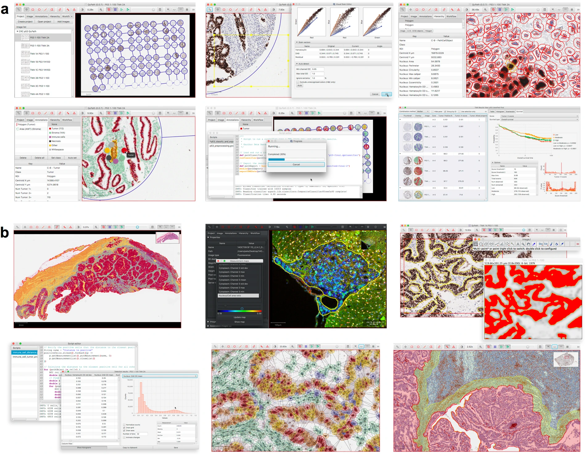
Qupath is a tool using machine learning to work with image analysis in the growing field of “digital pathology”. Scanners can quickly produce tens of gigabytes of image data of tissue slides, and traditional manual assessment is no longer suitable. As a result, automation through software provides a much faster solution.
In recent years, a vibrant ecosystem of open source bioimage analysis software has developed. Led by ImageJ, researchers in multiple disciplines can now choose from a selection of powerful tools, such as Fiji, Icy, and CellProfiler, to perform their image analyses. These open source packages encourage users to engage in further development and sharing of customized analysis solutions in the form of plugins, scripts, pipelines or workflows – enhancing the quality and reproducibility of research, particularly in the fields of microscopy and high-content imaging. This template for open-source development of software has provided opportunities for image analysis to add considerably to translational research by enabling the development of the bespoke analytical methods required to address specific and emerging needs, which are often beyond the scope of existing commercial applications.
Bankhead, P., Loughrey, M.B., Fernández, J.A. et al. QuPath: Open source software for digital pathology image analysis. Sci Rep 7, 16878 (2017). https://doi.org/10.1038/s41598-017-17204-5
Case Study: MicrobeJ
Website: https://www.microbej.com/
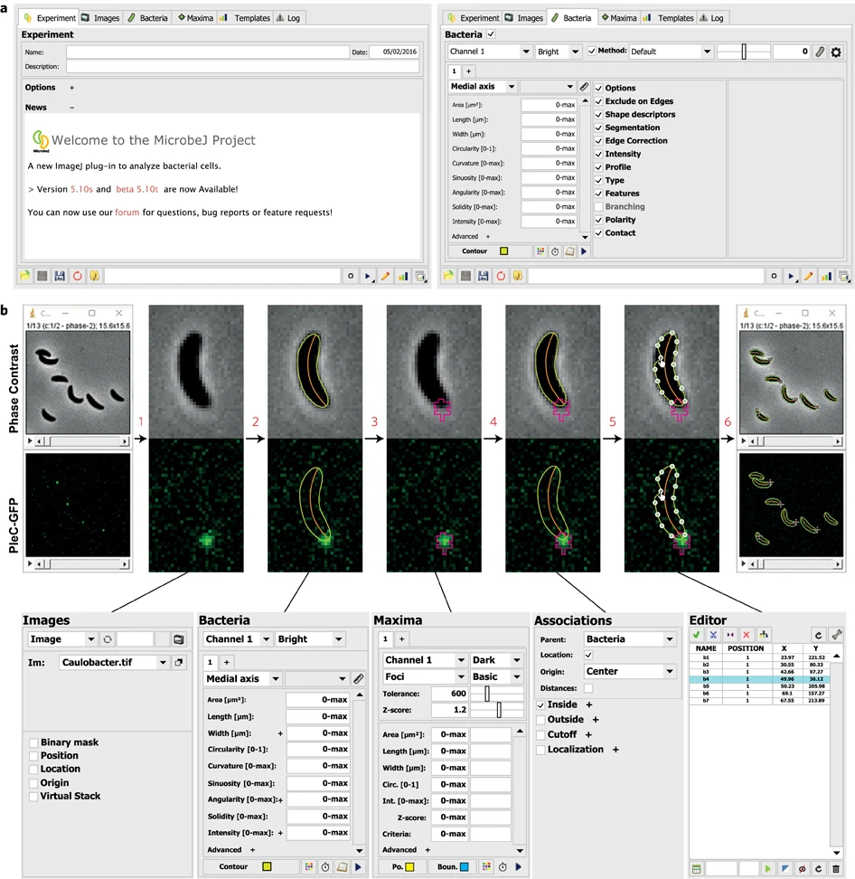
MicrobeJ is a plug-in for the open-source platform ImageJ. MicrobeJ provides a comprehensive framework to process images derived from a wide variety of microscopy experiments with special emphasis on large image sets. It performs the most common intensity and morphology measurements as well as customized detection of poles, septa, fluorescent foci and organelles, determines their subcellular localization with subpixel resolution, and tracks them over time.
Ducret, A., Quardokus, E. & Brun, Y. MicrobeJ, a tool for high throughput bacterial cell detection and quantitative analysis. Nat Microbiol 1, 16077 (2016). https://doi.org/10.1038/nmicrobiol.2016.77
Case Study: Cellpose
Website: https://www.cellpose.org/
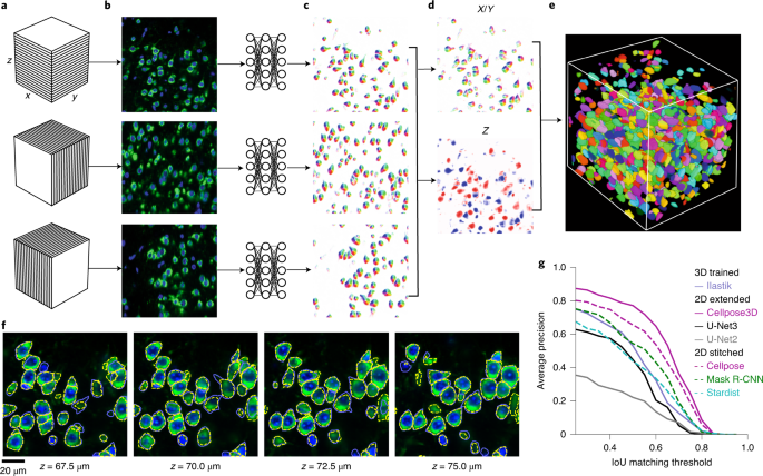
A generalist, deep learning-based segmentation method called Cellpose, which can precisely segment cells from a wide range of image types and does not require model retraining or parameter adjustments. Cellpose was trained on a new dataset of highly varied images of cells, containing over 70,000 segmented objects. We also demonstrate a three-dimensional (3D) extension of Cellpose that reuses the two-dimensional (2D) model and does not require 3D-labeled data. To support community contributions to the training data, we developed software for manual labelling and for the curation of automated results. Periodically retraining the model on the community-contributed data will ensure that Cellpose improves constantly.
Stringer, C., Wang, T., Michaelos, M. et al. Cellpose: a generalist algorithm for cellular segmentation. Nat Methods 18, 100–106 (2021). https://doi.org/10.1038/s41592-020-01018-x
Case Study: DeepLabCut
Website: http://www.mackenziemathislab.org/deeplabcut // https://github.com/DeepLabCut/DeepLabCut // https://deeplabcut.github.io/DeepLabCut/docs/standardDeepLabCut_UserGuide.html
Quantifying behaviour is crucial for many applications in neuroscience, ethology, genetics, medicine, and biology. Videography provides easy methods for the observation and recording of animal behaviour in diverse settings, yet extracting particular aspects of a behaviour for further analysis can be highly time-consuming.
DeepLabCut offers an efficient method for 3D markerless pose estimation based on transfer learning with deep neural networks that achieves excellent results (i.e. you can match human labelling accuracy) with minimal training data (typically 50-200 frames). We demonstrate the versatility of this framework by tracking various body parts in multiple species across a broad collection of behaviours. The package is open source, fast, robust, and can be used to compute 3D pose estimates.
Nath, T., Mathis, A., Chen, A.C. et al. Using DeepLabCut for 3D markerless pose estimation across species and behaviours. Nat Protoc 14, 2152–2176 (2019). https://doi.org/10.1038/s41596-019-0176-0
Exercises
- What tasks can be automated (and how) in your research workflow?
- Which of the presented use cases could be applied in your own experimental setup? If not, why?
Key Points
Despite not being at the cutting edge of AI development we can still benefit from elevated efficiency and accuracy of research data processing.
Examples of AI applications for automation include database search, image analysis and motion tracking
While not every researcher works with generating AI algorithms and models, there are plenty of tools with numerous applications in research that use machine learning. Automating tasks results in larger data sets and less manual work, and it is worth joining the online communities that work on the tools showcased here.
AI for Data Insights
Overview
Teaching: 0 min
Exercises: 0 minQuestions
How is AI used for data insights in biomedical experimental setups?
What types of data insights can be generated?
Objectives
Learning about examples of unsupervised and supervised ML applications in biomedical research
Adapting selected types of AI applications for data insights to inform your own research
Using AI in Research: Insight
We previously discussed using AI in tools for automating data such as data collection and classification. However, AI can also be used to give insights into data that is not posisble for humans.
Breakthroughs using AI in research are commonly discussed but should be considered with scepticism and a critical approach. In general, however, the ability for computers to process and analysis connections on a larger scale means it is possible for AI to find results.
We will discuss a range of examples.
Clustering: Letting the Machine Classify Data

Up until this point, we have looked at examples where humans have classified the data (handwritten digits, whether something counts as a cell, the difference between a duck and a goose) but a group of machine learning techniques called “unsupervised machine learning” does not use human labels, but can still find patterns in the data.
For example, by providing huge data sets and the connections between them, for example the “multiomics” of millions of cells, the machine can determine clusters within the data and how groups may be similar and disparate to each other. For this reason, machine learning classifications can provide insight into a dataset that would not be possible through human manual effort.
Using this kind of machine learning does not require a labelled data set, instead, the machine is allowed to find clusters using given parameters, such as how many it should find or how distinct groups need to be.
Xiao, Yi, et al. “Multi-omics profiling reveals distinct microenvironment characterization and suggests immune escape mechanisms of triple-negative breast cancer.” Clinical cancer research 25.16 (2019): 5002-5014.
Principal Component Analysis: When you have too many dimensions
Increasingly, with large datasets that cover the multiple -omics or collect hundreds or thousands of variables from biological specimens, it can be impossible to see the connections and interactions between them. Machine learning can help by collapsing down the complexity into manageable (but artifical) variables that sufficiently describe the data.
In principal component analysis, you could take some measurements of fish such as their length and height. By combining the data from hundreds of fish, you can use PCA to determine two new variables, which account for most of the variation in your dataset. The first is the scale of the fish (large vs small) and then the aspect ratio or “stubbyness” of the fish (stubby vs slender). You can use these two new variables, scale and stubbyness to describe the full variation in your data set, and so separate out your fish into:
- Stubby and large
- Stubby and small
- Slender and large
- Slender and small

Favela, Luis. (2021). The Dynamical Renaissance in Neuroscience. Synthese. 10.1007/s11229-020-02874-y.
Which is far more meaningful for understanding the morphology than separating out fish into bins of height and length values.
This example is simplistic because the data set only has two variables, but for data sets with hundreds of variables it can be very difficult to determine which variables are the most critical for understanding the diversity within your specimens. The combination of your variables into a principal component space can capture most of the variation in your dataset, and elucidate patterns that were not visible in the original data space.
Neural Networks: the black box
Neural networks can be used to infer predictions from data by learning from known examples. They are an example of “supervised machine learning”, unlike the previous examples, which means a large training dataset of labelled data is required before any predictions can be made.
If you have the a lot of different markers from one group of people who are known to have a disease and from another group of people without the disease, you can ask the machine to guess on a new series of people which group they may belong to. Or, you could build a neural network that learns the drug interaction effects on people with certain microbiome populations.
Case Study: Alpha Fold
Alpha Fold is a famous example of an extremely complex neural network approach to solving protein folding. It is not fully known how Alpha Fold works, but the gist is familiar, which is teaching itself how molecules interact with eachother by using a very large training dataset of known proteins.
Solving protein folding has been a hotly contested task. The predictive powers of machines in protein folding has not shown much improvement with less than 50% matching power in 1994, which improved to around 60% in the last decade. Alpha Fold was a game changer, with results of 90% last year.
How Neural Networks Work
How the machine makes these predictions is not very easy to unpick, which is why these methods are known as black box. We can therefore use a toy example from TensorFlow Playground to understand how they work.
With a very difficult dataset it can be impossible to know the “rules” behind what separates orange from blue.
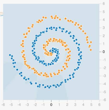
We start with a series of “properties”, or regions that could be used to classify the data. It is clear each of the following properties (regions) is not sufficient to classify our dataset.
![]()
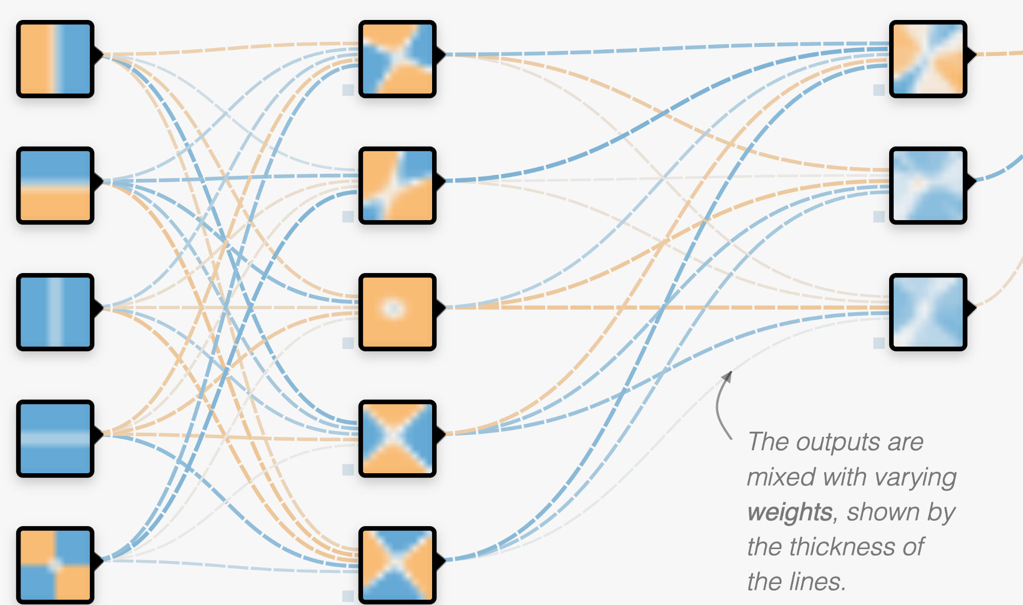
We can combine these regions together to make a new “layer”. The “neurons” in the neural network are combinations of the properties with varying weights (thickness of the lines). The model hasn’t learnt anything yet, and so the regions in this layer are currently randomised.
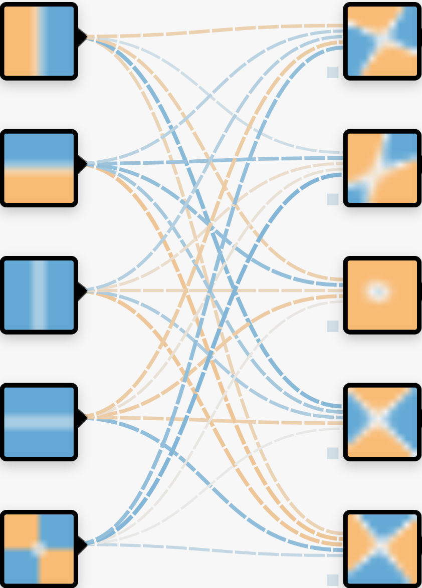
There is usually further layers which combine each of these with different weights as well. The number of these neurons can be vast, which is why it is difficult to know what is happening within the layers of the network or how they are defined.
Then, using the labelled training data set, the neural network rapidly alters the weights throughout the network to redefine itself. After it adjusts the weights it checks how well it is doing at classifying the data set, and adjusts itself accordingly to try and improve. Depending on the complexity of the take, this could take many hours or thousands of hours of computing.
Luckily, this toy example only takes a few seconds, so we can watch its progress.
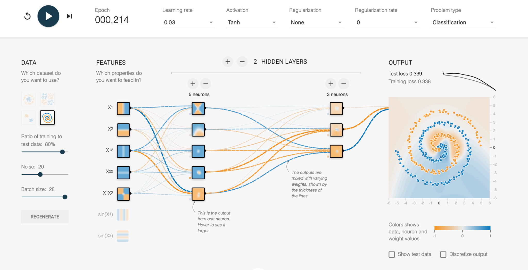
In the first increment, we see the vague blue and orange background as the network tries out its initial configurations. This is a start, where the middle of the data set is classified correctly, but the error is a high number (Test loss = 0.339 out of 1).
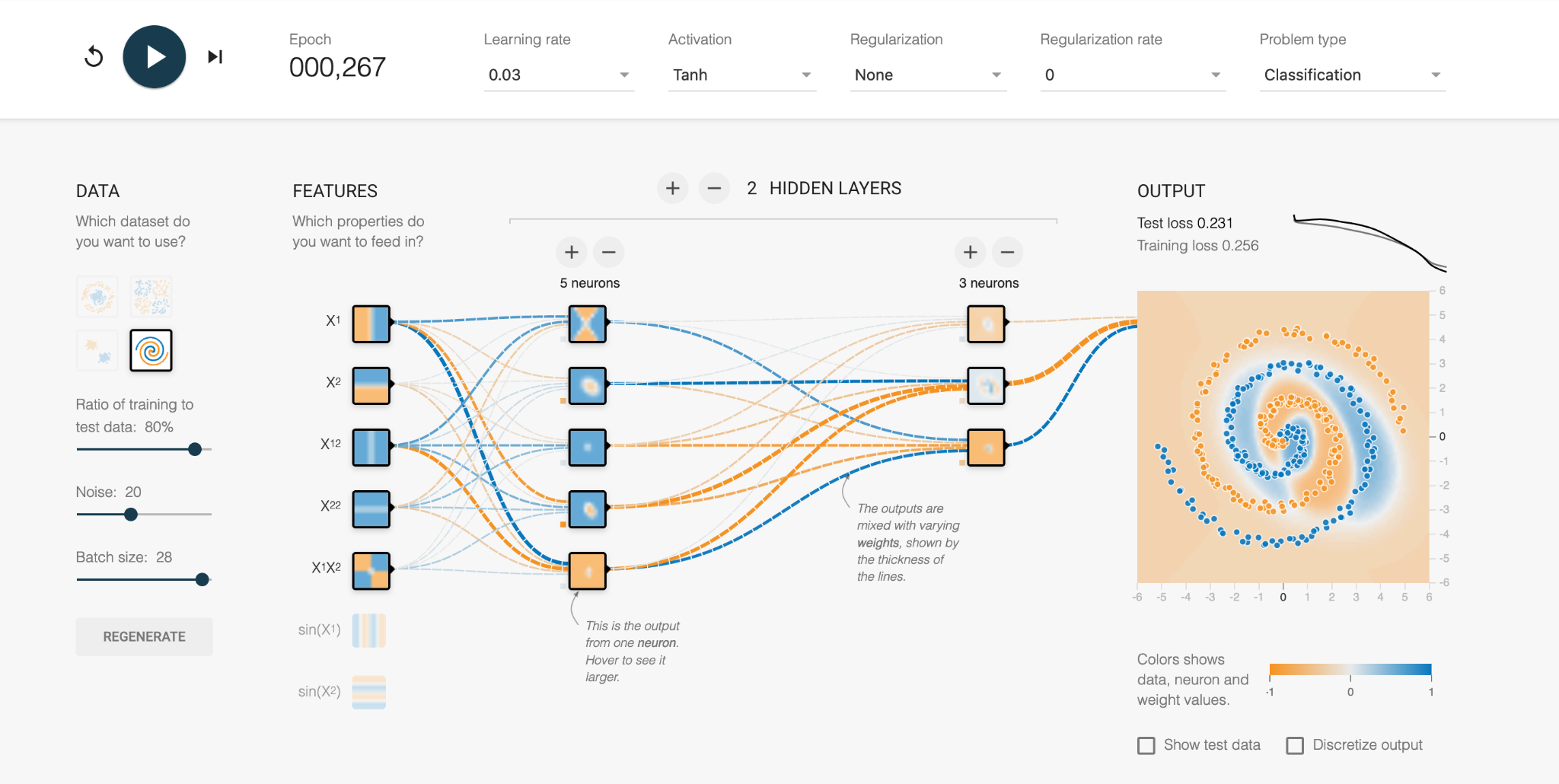
With further refinement, we can see the weights between the neurons are changed through trial and error, and the orange and blue regions more closely fit the actual data. The numerous mistakes mean the error is still high.
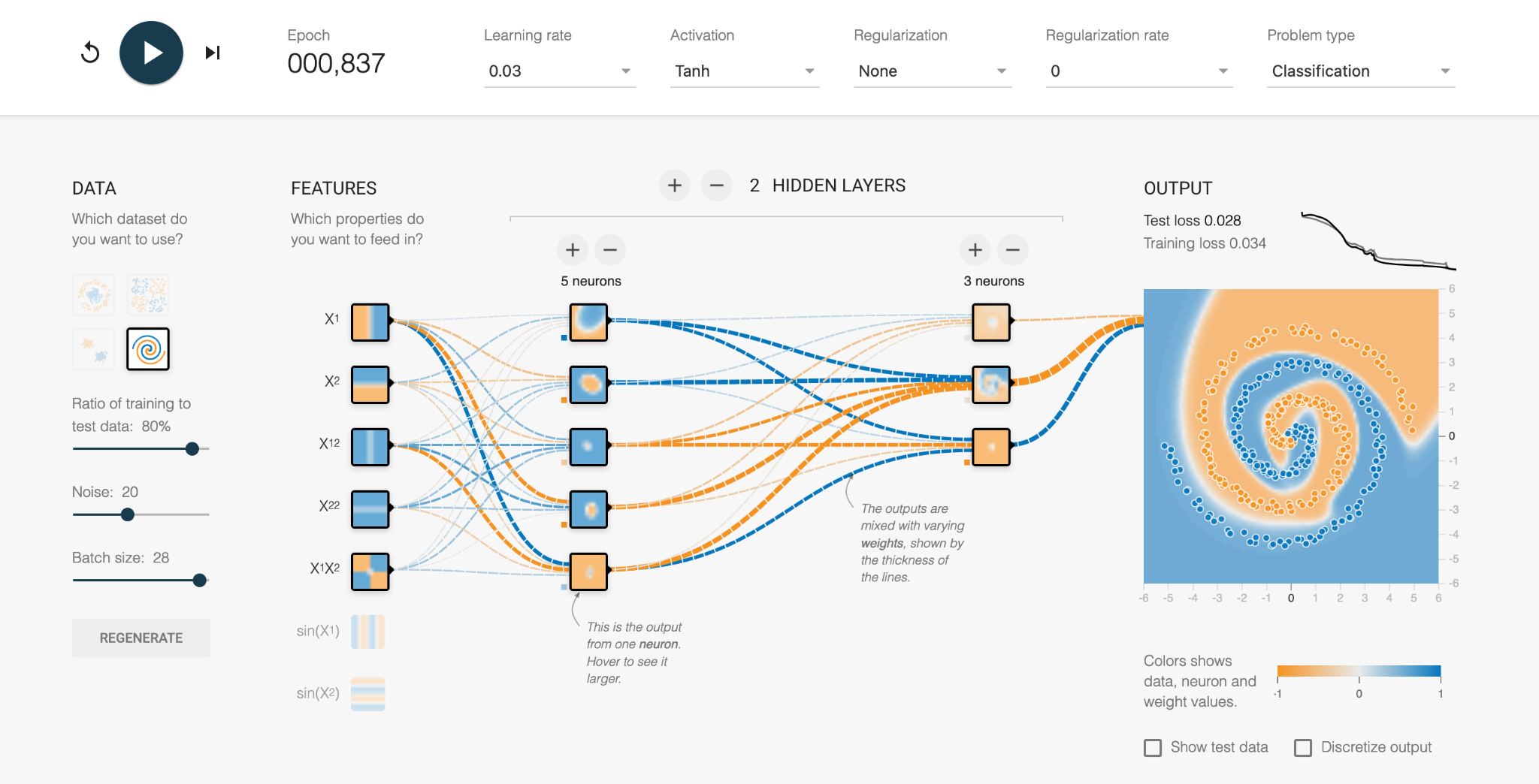
Eventually the network learns the complex boundary definitions of the two data types and produces a solution (Test loss = 0.028). We can look at each of the neurons and see what region it is personally responsible for, and whether it is -1 or +1 in the final combined solution.
It’s not usually this simple to “take a look” at the inner workings of a neural network, which is why a lot of scepticism and caution is required for using them, as discussed in the next episode. Interpretation and explainability of neural network predictions are very active areas of research.
Conclusions
Very large, multiconnected data sets can be too complex for humans to manually find insight, and so AI can step in and assist in more and more ways. Some methods are easier to understand and query than others, but using AI to assist human analysis is becoming a helpful tool in research.
Exercises
- What kind of data are you producing in your experimental setups?
- Which of the presented AI applications could further inform your research results interpretation?
Key Points
Very large, multiconnected data sets can be too complex for humans to manually find insight; hence AI can facilitate a scaled approach to data processing in various ways.
While some methods are easier to understand and query than others, AI applications can enhance human analysis.
Examples of A-facilitated methodologies for data insights include classification, clustering, and identifying connections in big data sets”
Problems with AI
Overview
Teaching: 0 min
Exercises: 0 minQuestions
What are the common pitfalls of using machine learning?
What are common limitations and pitfalls in ML applications?
What are conscious and unconscious biases that might influence ML algorithms?
How can data privacy and data security be ensured?
Who is responsible and accountable for any ethical issues implied by ML utilisation?
Objectives
Recognise the shortcomings and common problems with machine learning
Recognising the shortcomings and common challenges with ML algorithms
Knowing how to address and report common AI shortcomings
Being knowledgeable about responsibilities and accountabilities with regard to AI applications at your institute
Drafting a guideline to cover relevant ethical aspects in the context of your research field
Problems with AI
Limitations and ethical considerations of AI in biomedical research
When the Machine Learns Something Unexpected
The neural network used to distinguish wolves and huskies seen below got 8/10 of the following correct. The two mistakes are on the bottom row, the 2nd and 4th from the left.
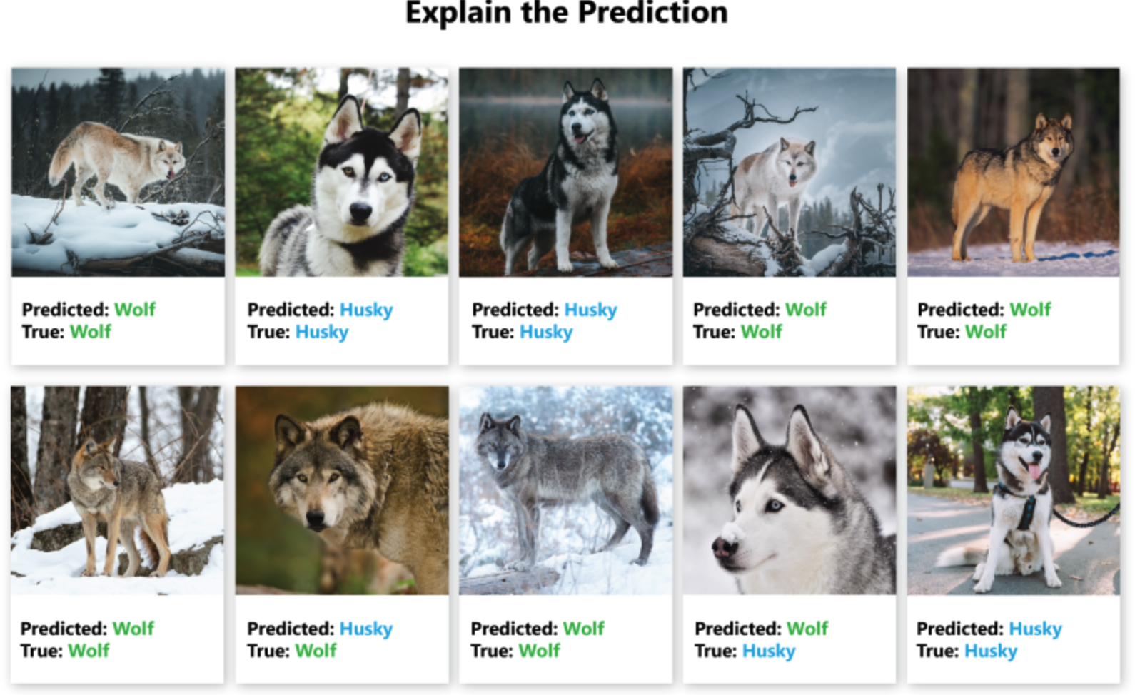
*Besse, Philippe & Castets-Renard, Céline & Garivier, Aurélien & Loubes, Jean-Michel. (2018). Can Everyday AI Be Ethical? Machine Learning Algorithm Fairness (English version). 10.13140/RG.2.2.22973.31207. *
We can’t easily see the neural network layers that explain how the model is distinguishing between wolves and huskies. However, for image data, we can use a pixel attribution method to highlight the pixels that were relevant for a certain image classification by a neural network. Here is another example of a husky falsely classified as a wolf by the neural network.

We can see the neural network is not using any of the pixels related to the canine, but instead looking at the background for the presence of snow to classify it as a wolf.
In the same way, the model may instead use unexpected and inappropriate signals in the data to provide an answer. A real-life example of this happened with a recent machine learning model used to distinguish cases of covid that were clinically severe versus moderate from X-rays, In the training data, the most severe covid patients were lying down during their chest X-rays, and so the model learnt to distinguish x-rays of people lying down.
Biased Data Leads to Biased Algorithms
Machine learning bias, also sometimes called algorithm bias or AI bias, is a phenomenon that occurs when an algorithm produces results that are systemically prejudiced due to erroneous assumptions in the machine learning process.
Where Does the Data Come From?
Data is not a natural resource, but the product of human decisions. Whether we are conscious of it or not, there are always humans involved when we speak about data creation. Data creation can be, for instance, collecting information or the tracking of historical information, organising information in specific categories, and measuring and storing information as data on digital infrastructure.
When we find a data collection enriched with metadata information or specific labels, we always need to remember that someone has either directly provided those labels or those have been automatically assigned by a tool trained on other manual labels.
To give a specific example, the famous ImageNet dataset, a central component for the development of many well-known image recognition pipelines in the last ten years, relies on two pillars: - a taxonomy developed since 1985 as part of the lexical database WordNet, which provides a top-down hierarchical structure of concepts (“chair” is under Artifact->furnishing->furniture->seat->chair) - an enormous amount of cheap workforce provided by Amazon Mechanical Turk. ImageNet is not an abstract resource, but the result of a gigantic effort and the specific representation of the World of 1) the people who have designed WordNet, 2) the researchers who have decided which WordNet categories are included and which are not in ImageNet and 3) the many, many annotators who have selected which images associate to concepts like “brother”, “boss”, “debtor”, “cry baby”, “drug-addict” and “call girl”, all included both in WordNet and ImageNet (at least until 2019).
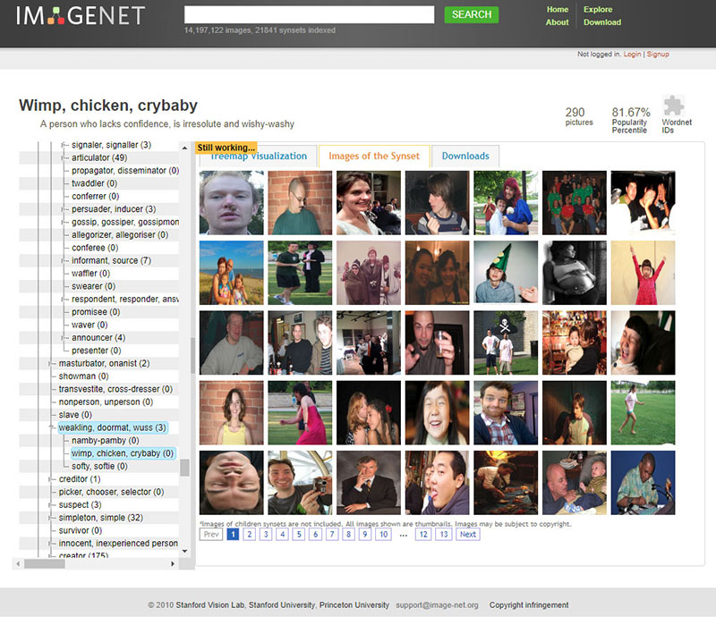
https://excavating.ai/
As researchers collect data that can go on to train machine learning models, there can be similar pitfalls. Labelling data sets can be open to human bias, where two people may differ on how to label a set of examples. In addition, even without human bias, there can be artefacts from how data was collected. In training a machine learning model to differentiate cancer tissue from normal tissue, if the cancer samples were all photographed from a lab in Germany and the controls were taken from a lab in Birmingham, the model may simply pick up differences in lighting and microscopes between the different data sets. It is therefore critical to consider the data that AI is using to train and where it came from.
Snake Oil: AI is not Magic
Professor Narayanan described how companies are using AI to hire candidates based on just a 30-second video. They dish out a blueprint with scores based on different aspects such as speech patterns that have been grasped from that video. These scores are then used to decide whether that candidate is a suitable hire or not.
Given enough data, a machine learning model can improve and be made reliable. However, in the case of ethical, and social dilemmas such as public policing or criminal prediction, anomalies emerge and can prove fatal.
Princeton’s Narayanan outlines the difference between AI innovations we can trust versus those we can’t:
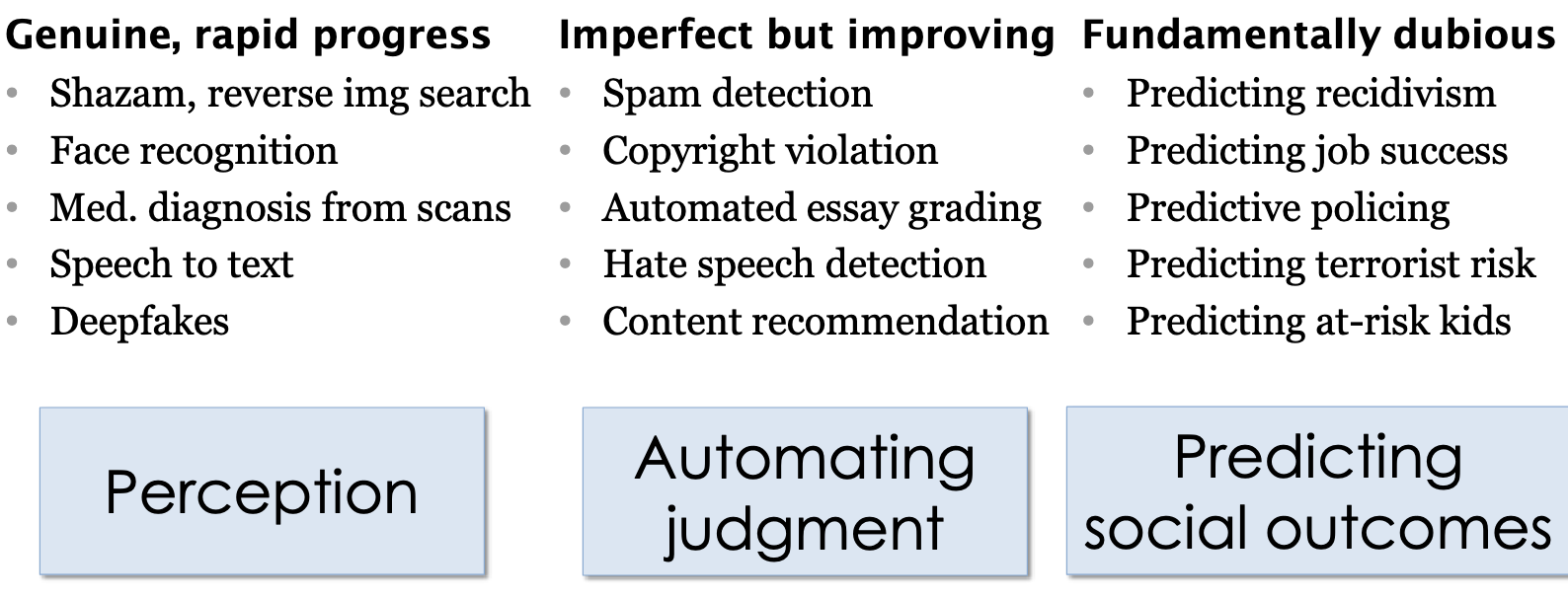
In the above cases, which are fundamentally dubious, as the professor likes to call them, the ethical concerns will be amplified with inaccuracies in model output.
In research, we are vulnerable to similar unfounded claims from machine learning, whether for describing new results or even applications to medical care. Approaching the results of machine learning with scepticism is important.
Read more: https://www.cs.princeton.edu/~arvindn/talks/MIT-STS-AI-snakeoil.pdf
Overfitting: Too Good to be Useful
A good machine learning model generalises well to data beyond its training data. When given data it has never encountered before, it creates sensible outputs. It is tempting to train a model so the error margins on the training data are minimal, but this leads to overfitting issues that we see in other statistical models.
Several techniques can help prevent overfitting. One way to avoid overfitting is to never validate a model using data from the training data set and to allow for some error in the model. Another way is to regularise the model, by encouraging simpler models that can capture most of the patterns within the training data, rather than complex models that can almost “memorise” the training data, which often provides poor predictions on unseen data. Other approaches look at selecting only a subset of important features contributing to the model performance.
Segmenting the data and repeating the training-validation process, for instance, via K-fold cross-validation, is a way to detect overfitting and optimise the parameters of an AI model. A combination of these techniques will likely be needed to effectively minimise overfitting and ensure the generalisation power of an AI model.
Further Reading
UKRIO: AI in research – resources
Exercises
- Think of examples in your research field, where AI applications might be problematic and lead to possible misinterpretation of the results
- Look through your institutional resources that provide ethical guidelines and define responsibilities
- Who might be authorities at your research institute that can be consulted and informed about ethical concerns about AI application?

Key Points
Machine learning should be used with scepticism to prevent biased results
We are vulnerable to unfounded claims from ML, whether for describing new results or even applications to medical care.
ML should be used with scepticism to prevent biased results.
A combination of data cleaning techniques is needed to effectively minimise limitations and ensure generalisation power of any AI model.
Beware of any biases and privacy/security concerns by enacting full transparency and accountability in the documentation and reporting of AI applications.
Practical Considerations for Researchers
Overview
Teaching: 30 min
Exercises: 20 minQuestions
What are the necessary steps before research data can be processed through ML pipelines?
What types of data cleaning can be applied to prepare raw data for ML?
Objectives
Understanding your data through Exploratory Data Analysis (EDA)
Gaining experience in data cleaning and preparation before running machine learning pipelines
Learning how to responsibly report AI-generated results
Practical considerations of conducting research with machine learning algorithms
Whether you are conducting your own research with machine learning (ML) algorithms, or reading about other work that has used them, there are some helpful ideas that can help you understand what work you might be undertaking or how to correctly interpret others’ research. This chapter aims to provide an overview of what is expected when such research and how results should be reported.
Data preparation is 90% of the work
If you are going to be building ML pipelines for your own research, then you should know that the vast majority of your time will be spent analyzing your datasets and preparing them for the (usually) few lines of code that will run your ML algorithm. So why is so much time often spent on data preparation?
You might be dealing with complex data structures
Depending on your research area, you will be in receipt of data that has been collected and curated in numerous different ways. If you work with data collected in a hospital setting, perhaps within one clinic you can expect to be working with excel spreadsheets fraught with multiple tables per spreadsheet, numbers interpreted as dates, and ad-hoc notes in random cells. Perhaps you might be more fortunate to work with a .csv file that contains one table per file. If you are working with more centralized data you will likely be working with relational databases that require you to merge tables together and aggregate them, usually with a database query language such as SQL.
If you are working with genetic data then you will have come across terms such as FASTQ, FASTA, BAM, SAM and VCF. These are all specialized forms of plain text files that contain various representations of genetic sequence data.
 |
|---|
| A FASTA file to contain nucleotide sequences. For whole genome sequencing expect millions of lines in such a file - the FASTA file for the human reference genome is ~ 3Gb in size. |
 |
|---|
| A Variant Call Format (VCF) File. All but the last 5 lines contain metadata about the file, and the “data” are only contained in the last 5 lines. |
It is probably not surprising that many of these file types are not directly usable with an ML algorithm, and code must be written to parse them into a format that can. We haven’t even touched on the fact that image and unstructured text (e.g., in natural language processing) are often sources of data for ML pipelines. How would you send the words you are reading right now into an ML algorithm to decide if the source is fact or fiction? How do you parse image data, a grid of pixels split into Red, Green and Blue channels into a .csv like structure?
 |
|---|
| Image data can be represented in various forms. Here the image is represented by three matrices: Red, Green and Blue, shown in the middle. Entries represent the intensities of pixels; Those matrices can be flatten and reshaped into an image vector. |
Data quality can be poor
Biomedical data is almost never collected for AI/ML algorithms, and most of the time not even for research. Most primary and secondary care is collected at point of care, and certain clinical codes (prescriptions) have monetary incentives for collection, but other (symptom tracking) do not. Lab tests are only reported to provide care to patients. Even if downstream research is kept in mind during data collection, are data standards in place such as data dictionaries that multiple sites can follow?
The variable nature of data quality mainly falls into two categories: systematic and random error.
Systematic errors are the weakness of oversight in methodological design or execution. Examples might include:
-
Research units submitting genetic data to a consortium might be using different sequencers or reference genomes. How do we harmonize the inherent differences in output data that will arise?
-
There are a disproportionate amount of a certain group of people in a cohort study. If we are predicting risk of an event in the population, how might this skew our results and how do we correct for this?
-
Missing data or incongruous data being collected due to poorly set out guidelines for field staff.
-
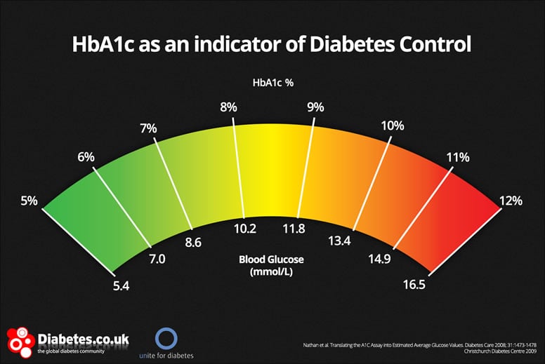
HbA1c is commonly reported on two different scales (m/mmol and %) that share a very similar value distribution. What if one field researchers are using different scales? This is incredibly difficult (likely impossible to disentangle).
Random errors are those that occur due to chance and usually cannot be accounted for at the point of collection, but only through correction or “cleaning” after that data has been collected. Human error in data collection is the most easily understood source of random error, but also medical equipment, sequencers, image software all have some source of random error. Examples of random error might include:
-
Clinicians might enter an incorrect prescription date or blood pressure value. Could we using a limit of normality to detect infeasible blood pressure values in a patient record? The author writing this chapter has worked with primary care databases that accidentally replaced the BMI column with today’s date i.e. a BMI of 20222104!
-
Patient identifiers such as NHS number are incorrectly entered and therefore “sharing” medical events with someone else in error. This can result in people appearing to have died and then pick up their hayfever prescription a month later, or people assigned as male on their birth certificate going on to give birth multiple times.
-
A clinician mistypes the word “epilepsy” as “eplispey”. Can ML algorithms deal with misspellings to determine people who are suffering from epilepsy?
Fantastic errors and where to find them
Between dealing with complex data and the errors that they might contain you will need to ensure that as much error has been removed as possible and you harmonize your data into a “final” dataset that can be passed to an ML algorithm. The saying “garbage in, garbage out” is exactly the situation we are trying to avoid when we send data into an ML algorithm. Exploratory Data Analysis (EDA) largely accounts for a type of (usually automated) analysis to pick up errors in your data. For example, a quick visualization of data, using one line of code from a cardiology clinic shows that some people have cholesterol values of zero:
featurePlot(x=data[1:7,], y=disease_status, plot="density")
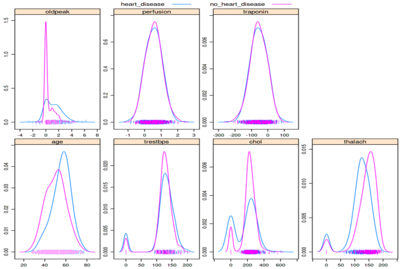
Can you spot the bimodal peaks in the “chol” and “trestbps” features? These zero values likely indicate these data weren’t collected or not entered and leaving the values as zero can greatly skew the results of any analysis, including training an ML algorithm
A simple density plot like the one above can be very effective at quickly spotting discrepancies, including values that are extreme such as 0 or a blood pressure of 999. It should be stressed though that these types of errors are quite easy to detect and are usually found during a first pass of the data. Some of the previous sources of error we have discussed can be far more difficult to spot - the example of incorrect input of an NHS number is particularly nasty given that the data doesn’t look extreme unless you are looking for people that have died and then seemingly come back to life. The only way to discover issues with your data is to spend time querying it and trying to anticipate what might arise. Over time you will want to develop unit tests that automatically test for such errors in your data, and this is where a lot of the time is spent in the data preparation phase.
Dealing with missing data
Missing data is a common challenge in data analysis that arises when information is absent for certain observations or variables. This missingness can occur anytime during the project or data lifecycle, such as during data collection, manual data entry or poorly designed data collection/reuse plans. Tools like data visualization, summary statistics and Python/R scripts to detect/identify gaps in data can help spot and visualise missing values. Any missing information from the data set used in the project should be reported through appropriate documentation.
We won’t be diving into this topic, but encourage our learners to check out the following learning resources to understand different kinds of data missingness and how to best handle them in their projects:
- Heymans, Martijn W. and Jos W. R. Twisk. “Handling missing data in clinical research.” J. Clin. Epidemiol., vol. 151, 1 Nov. 2022, pp. 185-8, doi:10.1016/j.jclinepi.2022.08.016.
- Effective Strategies for Handling Missing Values in Data Analysis, Nasima Tamboli, Analytics Vidhya
Exercises
- What are the kinds of raw data in your research and how do they need to be prepared for ML Applications?
- Which steps in the presented data preparation workflow can you apply to your research?
Key Points
90% of Machine Learning is data preparation.
It is easy to misrepresent machine learning results.
Learning techniques such as building confusion matrices, ROC curves, and common metrics will help you interpret most ML results
Practical Considerations: Reporting Results
Overview
Teaching: 30 min
Exercises: 20 minQuestions
How do research results differ with regards to Supervised versus Unsupervised Learning?
What are best practices for responsible reporting results from ML pipelines?
Objectives
Understanding typical outputs from supervised and unsupervised ML algorithms
Knowing how to present ML-derived results responsibly
Reporting results from machine learning pipelines
As with any other statistical analysis you can expect to report various metrics that communicate your results obtained from a machine learning (ML) pipeline. You may have heard of p-values, adjusted R-squared and the t-statistic used in methods such as a t-test or chi-squared-test. Supervised (regression and classification) and unsupervised ML algorithms have distinct metrics that you will be reporting:
- Supervised algorithms:
- Accuracy
- Sensitivity
- Specificity
- Precision
- Recall
- F1 score
- Mean Squared Error (MSE)
- Root Mean Squared Error (RMSE)
- Mean Absolute Error (MAE)
- Unsupervised algorithms
- Total within sum of squared error
- Gap statistic
- Silhouette value
- Akaike Information Criterion
Reporting results in regression (supervised)
While there are many techniques that fall under the term “regression” such as linear/multiple, logistic, poisson or Cox proportional-hazards, they all aim to fit a line of best fit to the data, and so here we describe metrics that relate to describing how “good” a line of best fit is.
Most regression metrics are derived from a “residual” - the distance of a line of fit to a data point. Some some data points fall below the line of fit and some fall above the line of fit, so to ensure the residuals don’t cancel out, we take the square of the residual and arrived at the “sum of squared residuals”.
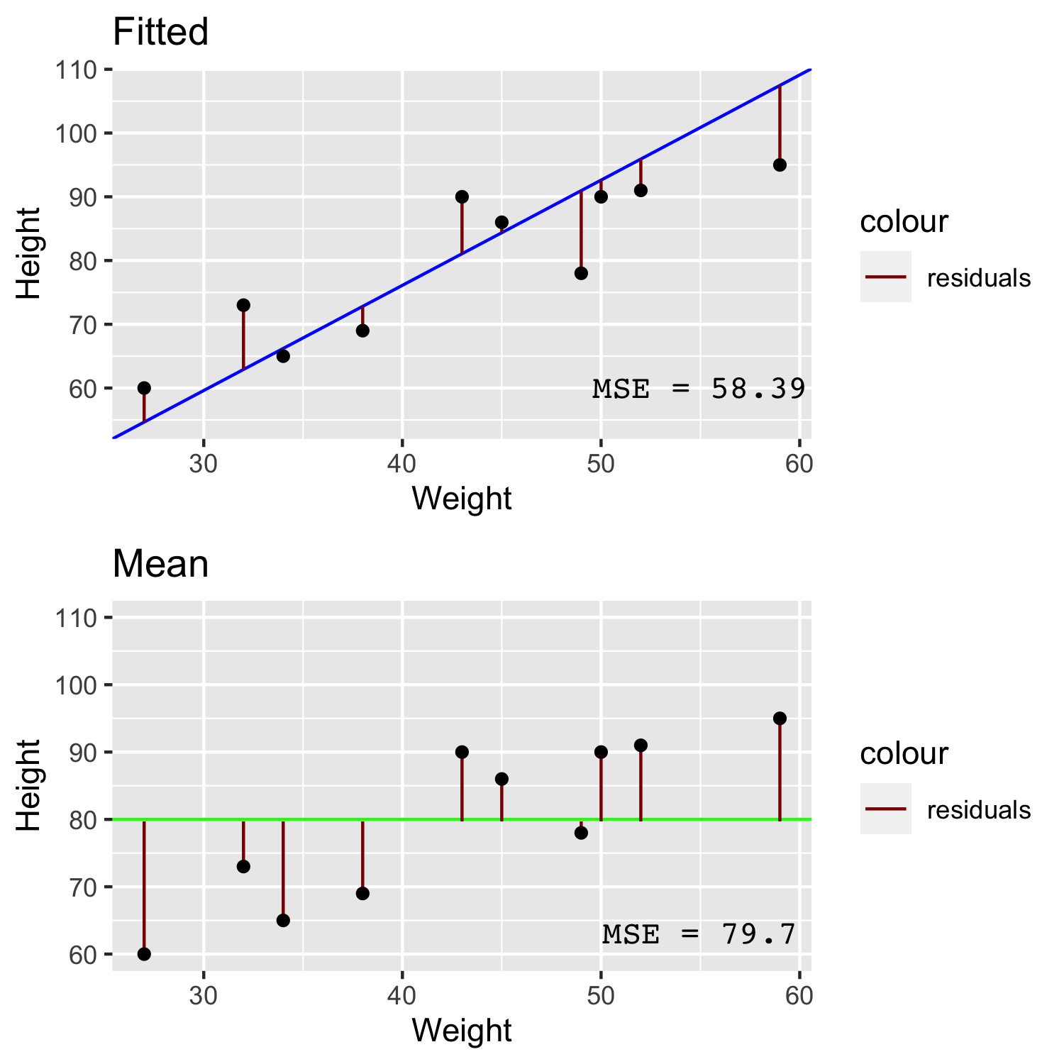
In the image above we can see that for a line that has been fitted to the data with linear regression (blue) has quite small residuals (red) compared to the larger residuals of a line comprised simply of the mean height (green). The Mean Squared Error (MSE) is simply the sum of squared residuals divided by the number of data points. By taking the root of the MSE we get the Root Mean Squared Error (RMSE). If you were to take the absolute value of the residual instead of the squared residual then you will arrive at the Mean Absolute Error (MAE).
You might point out that each of these three measures appear quite similar, however if you consider that case of having a higher number of outliers, the RMSE or MAE are better metrics to use over MSE because the MSE will be inflated due to squaring the large residuals of outliers.
Reporting results in classification (supervised)
Supervised learning can be divided into two types of problems: regression and classification. Regression is used for the prediction of continuous variables, and classification aims to classify something into specific categories, and often into just two categories (binary). Here, we mainly focus on classification tasks.
When training a supervised algorithm we can compare its predictions to the ground truth and therefore say if it is correct or incorrect. These leads to the first staple of reporting in supervised learning: the confusion matrix.
Training, Testing and the Confusion matrix
When we report results from supervised classification, we are only interested in calculating metrics from the test data - the training data is used only to train the model. From the test data, we can use our trained model to make predictions and compare to the actual classes of each item in the test set. For N number of classes (e.g. N=2 for predicting cancer vs no cancer), a confusion matrix is an NxN matrix that records how many the algorithm classified correctly and incorrectly by visualizing the actual classes against the predicted classes.

However many classes there are, a confusion matrix reports 4 types of outcome:
- True Positives - The classifier predicts a positive case i.e. cancer, and that person does actually have cancer.
- True Negative - The classifier predicts a negative case i.e. no cancer, and that person doesn’t actually have cancer.
- False Positives - The classifier predicts a positive case i.e. cancer, but that person doesn’t actually have cancer.
- True Positives - The classifier predicts a negative case i.e. no cancer, but that person does actually have cancer.
These 4 components can be used to calculate the most common metrics in supervised classification: accuracy, sensitivity and specificity.
- Accuracy - The percentage of correct classifications in the dataset.
- Sensitivity - The percentage of positive cases correctly identified. Sometimes called the True Positive Rate (TPR).
- Specificity - The percentage of negative cases correctly identified. Sometimes called the True Negative Rate (TNR)
Performance metrics are problem-dependent. For example, if your primary aim is to pick up as many COVID-19 cases as possible to reduce spread, sensitivity will tell you how well your algorithm does, not accuracy. If it is important to be as sure as possible that someone will likely develop disease because it will likely cause harm in other ways i.e. developing mental health issues due a diagnosis of dementia, specificity can help you prioritize when to label someone with the disease. Therefore, it is important to know how to trade sensitivity with specificity. This is where the Receiver Operator Characteristic (ROC) Curve can help.
In some use-cases, such as information retrieval tasks, a task where you want to retrieve relevant documents or records from the population, we often talk about the precision and recall of a model rather than specificity and sensitivity. For example, if we wrote an ML algorithm to scan clinic letters for people with epilepsy, we know that most of the population do not have epilepsy and so “no epilepsy” won’t be explicitly recorded. The recall is described by out of all the possible epilepsies in the population, what percentage does the algorithm pick up? This is exactly the same as sensitivity! This tells us the model’s ability to recall as many epilepsies as possible from the population. However, we can also ask how many of just the people in the population who have known epilepsy, how many are identified as such by the model? This is this precision of the model and unlike recall being the same as sensitivity, precision is not the same as specificity.
K Crossfold Validation
Instead of using a simple train/test split to report our results, it is common to use a method called crossfold validation. Here we can split the data into X% training data and Y% for test data (an 80/20 split is quite common) K times (K=10 is also quite common). Note that when we talk about K crossfold validation the “test sets” in each fold are called validation sets. The reason for doing K crossfold validation is because if we only chose K=1 it might turn out that the test data by chance contains some unrepresentative data points compared to the data as a whole (or more importantly in a real world population scenario). So by repeating the sampling process we aim to use all data point in at least 1 test set. Another reason to do this is to help select the best hyperparameter values during training (again, we might get lucky or unlucky with just one training set).
But there are two extremely important things to remember when using K crossfold validation. The first is that we only ever split the training data up into subsequent K splits i.e. we should always hold out a completely separate test set that never gets used during crossfold validation and biases the training process. Therefore you should think of K crossfold validation as something that happens during training. This leads onto the second important thing to note: the validation sets from each fold are not your final results - they are merely there to show you how stable a model is and to find the best hyperparameter values. Once we know our values and stability we discard all of the individual folds and re-train our model with all of the training data, and then use the held out test data to report our results.
The following diagram should help you visualize an ML experiment that used K crossfold validation:

ROC Curves
In addition to predictions (e.g. “disease” or “not disease” labels), some ML algorithms provide a numerical score (in some cases a probability) that measures the quality of the prediction. Whatever this numerical range is, we can choose a threshold of when to classify someone as having a disease. If we move the threshold one way we will increase sensitivity, and if we move it the other direction we will increase specificity. This means we could visualize all the resulting sensitivities and specificities for each threshold we choose. This powerful visualization is called a ROC Curve and we can use it to choose a threshold for a desired sensitivity, knowing how much specificity we would have to sacrifice.
| <p align="center">
 </p> |
| :–: |
| Receiver Operator Characteristic (ROC) Curve. The y-axis shows True Positive Rate (TPR), also called sensitivity or recall. The x-axis is False Positive Rate (FPR) or 1 - specificity. The ROC curve plots the FPR against TPR for various thresholds, i.e., the points along the blue curve.|
</p> |
| :–: |
| Receiver Operator Characteristic (ROC) Curve. The y-axis shows True Positive Rate (TPR), also called sensitivity or recall. The x-axis is False Positive Rate (FPR) or 1 - specificity. The ROC curve plots the FPR against TPR for various thresholds, i.e., the points along the blue curve.|
The orange dashed line shows the ROC curve of a purely random classifier. For such classifiers, sensitivity = 1 - specificity (or TPR = FPR) at all points. The blue curve shows the TPR vs FPR at all threshold values, and the closer a ROC curve is to the top-left of the graph (TPR=1, FPR=0) better. We can also calculate the Area Under the Curve (AUC) that allows us to see the total aggregated measure of TPR and FPR over all thresholds and is often reported along with accuracy.

With consideration to the orange “line of chance”, we can draw the opposite (black line), where this line crosses the ROC curve and is the point that the default confusion matrix is calculated from. However, if we move the threshold, we can obtain a different confusion matrix. From the blue curve we have marked a further point on the graph - one that trades away some specificity for an increase in sensitivity. This point will provide us with different values in our confusion matrix in which we will see more True Positives, but also more False Positives.
Calibration of predictions from over or under sampled datasets
ROC curves are most effective when we have equal proportions of the classes i.e. balance. Most situations are not balanced i.e. only 1% of people have epilepsy, and so we need to be interested in optimizing on both sensitivity and precision (which of those classified as epilepsy are actually epilepsy and how many of the possible epilepsies can the algorithm detect). We can swap out the specificity (False Positive Rate) in the ROC Curve for precision and re-plot. This is more commonly known as a Precision-Recall Curve, where Recall is just another term for sensitivity or True Positive Rate.

In the previous chapter we considered approaches to deal with imbalanced data - namely random undersampling and SMOTE to improve accuracy. This gives rise to a problem in that these methods can greatly effect predicted class probabilities, and you might only be interested in the class probability rather than the binary decision (this is far more useful in the author’s opinion!). Logistic regression is a perfect example - it is just a regression technique until you impose a threshold of class probability to classify into a binary outcome. It is entirely possible to have a good “classifier” but still have strange predicted class probabilities i.e. after oversampling the majority class, the predicted probability profile distribution of healthy controls are artificially shifted closer to that of those who went on to develop some disease, but an appropriate threshold might still be able to discriminate between both groups well. The problem is that you could end up telling someone who might not ever develop the disease that they have a high probability of developing the disease, even though the class label predicts them not to develop it. Is there an all purpose method to ensure whatever probabilities the model outputs, we can assess and calibrate them to what we expect in the population?
#####The Brier Score
The Brier Score compares the difference (mean squared error) between the predicted probability distribution. We can quickly see if a model is over-estimating or underestimating risk in the population.

We can see that the random forest classifier in the above image is not well calibrated to the reference (black dotted line) as it deviates far away at very low and very high probabilities, indicating that the model is favouring scoring someone as either very low risk or very high risk. In comparison the logistic regression model is better calibrated and more likely to predicted risk in those other than clear cut low or high risk (which in some cases describe the population accurately, hence an accurate classifier even though it is poorly calibrated). However, if your model is poorly calibrated you can scale the predicted probabilities using methods such as Isotonic Regression and Platt Scaling.
Here are two interesting resources on risk calibration and the role of thresholds for classification: https://bmcmedicine.biomedcentral.com/articles/10.1186/s12916-019-1466-7 https://www.fharrell.com/post/classification/
Reporting results in Unsupervised analysis
While Supervised learning focusses on optimizing metrics such as accuracy, sensitivity and specificity, Unsupervised learning doesn’t have the ground truth to compare predictions to. As mentioned in previous chapters, the aims of unsupervised learning is to allow an algorithm to find hidden groups, or clusters from the dataset and therefore we are interested in providing metrics that show us an appropriate number of hidden clusters.
Total Within Cluster Sum of Squared Error
Most algorithms require you to run the cluster analysis with different values of K, the number of clusters, and then calculate the error within each cluster by measuring the squared (and square rooted) distance between the each datapoint and it’s cluster center. We take the square root of the squared distance to avoid adding minus numbers. For example if we run the algorithm with 4 clusters we can calculate the error for each cluster, and sum them to get the total within cluster sum of squared error.
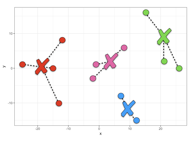
It is up to you to try out different values of K and then comparing the total within cluster sum of squared error in which you are trying to find the value of K that minimizes the error. What values of K should be tried? Firstly it is pointless trying K=1 because you have not learned anything from the data. Secondly you would not set K=N, the number of datapoints because while this would end up with zero error (each datapoint is it’s own cluster so 0 distance between them), we also don’t learn anything. There needs to be a preferable range that is usually between K=2 to K=10. This may change in some cases e.g. using cluster analysis to determine how many unique patient pathways there might be for starting medication following a diagnosis - there are only a finite number of treatment regimes and so K would at least be limited by that upper bound. Once you have decide a range you will want to visualize your results
Elbow plot
A common visualization of error analysis in unsupervised learning is the Elbow Plot. We plot K vs the total within sum of squared error and look for the “elbow” - the point at which error has reduced sufficiently before it begins to plateau within increasing K.
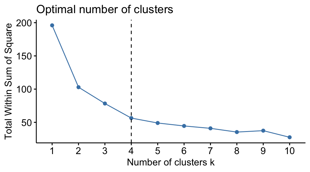
As you can see, because there isn’t a nice upper bound to aim for such as 100% accuracy, choosing the optimum value of K is more open to interpretation. Sensible choices appear to be in the range of 2-4, in which it is up to you and your team of experts to discuss what the implications of splitting your cohort of patients, genes etc into 2-4 groups.
We could also plot the cluster membership against various features in the data. In the figure below, with K=3 we can see that the 3 clusters separate well across the feature “Flavanoids”, but not across the feature “Ash”, indicating that Flavanoids is an important feature in the clustering process.
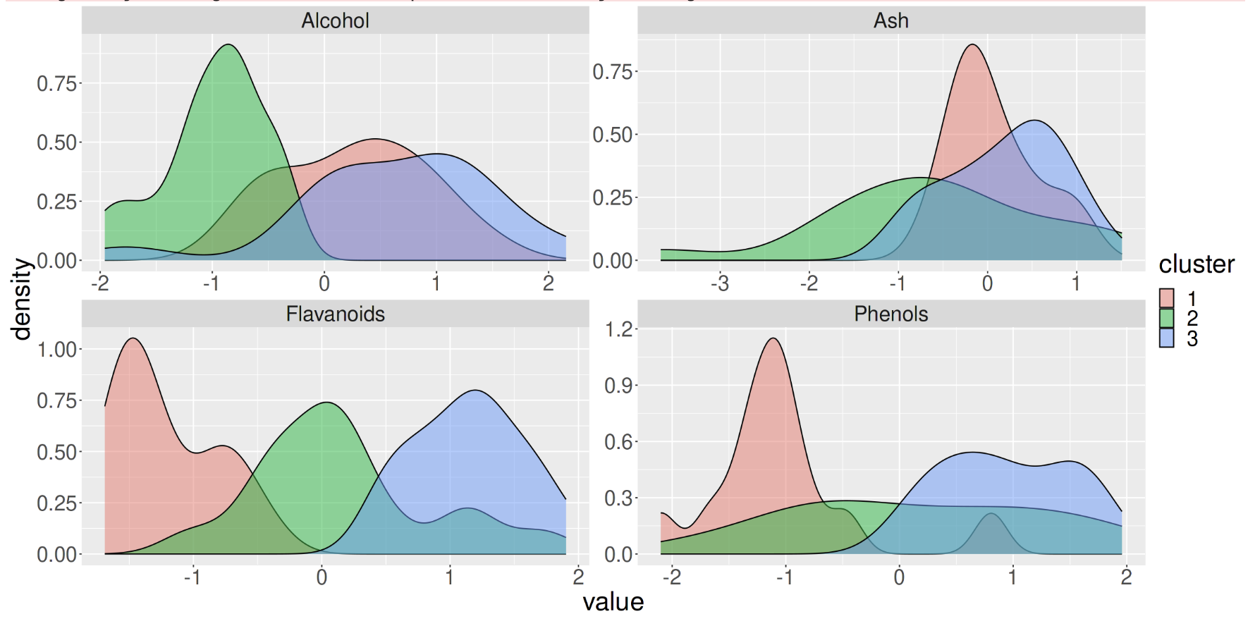
It’s at this point that the results of unsupervised analysis can be carried out with metrics just as in supervised analysis, but also should involve some form of Exploratory Data Analysis (EDA) to help you determine what are the optimum number of clusters for your purposes.
Conclusions
Just like any other statistical analysis, ML results comprise of presenting certain metrics to assess the utility of a model. Supervised learning optimizes against a ground truth and so we can use metrics such as accuracy and sensitivity where the goal is to achieve 100% in such metric. Unsupervised learning is more nuanced because we don’t have aground truth - while we optimize against the total sum of squared error (and the many other variations on this theme), we often have to rely on exploratory analyses in conjunction with our use case to decide what an optimum number of clusters are.
Exercise
- Discuss with your colleagues which of the Supervised and Unsupervised Analyses might be applied to answer a research question in your field.
- What are the respective limitations and possible misinterpretations?”
Key Points
Just like any other statistical analysis, ML results comprise of presenting certain metrics to assess the utility of a model.
While Supervised Learning focusses on optimizing metrics such as accuracy, sensitivity and specificity, Unsupervised Learning is used to find hidden groups.
Supervised learning optimizes against a ground truth and so we can use metrics such as accuracy and sensitivity where the goal is to achieve 100% in such metric.
Unsupervised learning is more nuanced because we don’t have a ground truth - while we optimize against the total sum of squared error (and the many other variations on this theme), we often have to rely on exploratory analyses in conjunction with our use case to decide what an optimum number of clusters would be.
Common frameworks can be used to present your work and ensure they are consistent within ML-facilitated research.
ML intends to deploy a model in a real-world setting and as such you should report its predictive power and limitations accurately.