Organizing Camera Trap Data
Overview
Teaching: 60 min
Exercises: 30 minQuestions
How can we use program R and package camTrapR to organize camera trap data?
Objectives
Perform camera trap organizational steps like renaming files
Extract exif data from camera traps
Combine dataframes with locational information
In camera trapping studies, it’s common to have a lot of camera photos, sometimes thousands or even millions of images that need to be processed and formatted for analysis tasks. Camera trap data organization requires careful management and data extraction that can be greatly assisted by the use of programming tools, like program R and Python.
In general, if we want to organize our data from raw camera trapping data, there will also be other files including GPS locations, and camera operations data including start-times, end times and any issues encountered that may have interrupted camera data capture such as repairs.
We will begin this module by first organizing and formatting our camera trap data that have already been sorted for the snow leopard species. Our goal is to sort these images by individual, and so our first steps will be processing and organizing the raw camera trap information.
First, set the working directory for the workshop where the snow leopard data have been downloaded, which is essentially a folder of your camera trap imagery.
#Set working directory
setwd("YourWorkingDirectory/CarpentriesforCameraTraps/")
#Make sure to have ExifTool installed and bring in the camtrapR package
library(camtrapR)
Set the file path of your image directory
# raw image location
wd_images_raw <- file.path("2012_CTdata")
One of the first steps that we want to perform is a data quality check. Make sure that each of the file folders has the name of the camera trap station, often including the name and number. In our case we have cameras with names like “C1_Avgarch_SL”, which indicates that this camera station was numbered 1, and at a location named Avgarch. These names are consistent across data tables such as the GPS coordinates and camera operations information, making it easier to merge this information.
Since SD cards often name files sequentially like “IMG_1245.jpg”, then there may be more than one file with this name within the multitude of camera trap photos we have captured. Our goal is to give each image a unique filename that uses the location, date/time, and a sequential number, so that the photo filenames are unique. To do this, the folder names have to have the location information because the new image names will have the camera trap location as an identifier.
To create a new directory for our copied data we can use the dir.create function.
In our case, we will name the new folder 2012CameraData_renamed
#create directory
dir.create("2012CameraData_renamed")
Then, set the file.path to an object, which eventually will be used for adding the renamed images.
#get the file path for the new directory and store in an object
wd_images_raw_renamed <- file.path("2012CameraData_renamed")
A quick fix before we rename. Some camera trap models (like Reconyx) do not use the standard Exif metadata information for the date and time, which makes it not possible to read directly, so we use the fixDateTimeOriginal function in the camTrapR package.
#fix date time objects that may not be in standard Exif format
fixDateTimeOriginal(wd_images_raw,recursive = TRUE)
Renaming camera trap files is possible using the imageRename function. Here we specify the input and output directories.
There are additional parameters for whether the directories contain multiple cameras at the station, like an A and B station opposing each other (hasCameraFolders). In our case, our folders do have subdirectories, but they are not specific to a substation, so we will set this to false.
Additional parameters include whether the camera subdirectories should be kept (keepCameraSubfolders), and we do not have extra station or species subdirectories we can also keep this as FALSE. We will set copyImages to TRUE because we want these images to go into a new directory.
#rename images
renaming.table2 <- imageRename(inDir               = wd_images_raw,
                               outDir              = wd_images_raw_renamed,
                               hasCameraFolders    = FALSE,
                               keepCameraSubfolders = FALSE,
                               copyImages          = TRUE)
Next, we will create a record table or dataframe of the exif information, that includes station, species, date/time, and directory information.
If you followed the setup instructions carefully, then you should have no issues with ExifTool which has the backbone tools for extracting exifs. However, you may need to install it. https://exiftool.org/
First you can check if you have the tool installed:
Sys.which("exiftool")
If not, then you can configure it using the path information for where the tool was placed on your computer. It does not need installation, but it does need to be found on your computer.
# this is a dummy example assuming the directory structure: C:/Path/To/Exiftool/exiftool.exe
exiftool_dir <- "C:/Path/To/Exiftool"
exiftoolPath(exiftoolDir = exiftool_dir)
Moving onto our exif extraction. There are parameters to allow the extracted exif dataframe to include available species information, to be sorted from the directory, for example your data may be sorted with this structure: (Station/Species) or (Station/Camera/Species). In our case, we only have one species, snow leopard images, so we will not use these extra settings, although the parameters are available if your data has species folders.
#create a dataframe from exif data that includes date and time
rec.db.species0 <- recordTable(inDir  = wd_images_raw_renamed,
                               IDfrom = "directory")
After inspecting the dataframe, we can see there is a Species column with the wrong information in it, so let’s tell the dataframe which species and genus we are working with.
#change the species column contents
rec.db.species0$Species <- "uncia"
rec.db.species0$Genus <- "Pathera"
To save this table to a csv file we can write this to file, so we have the raw exif data if we need it.
#write the Exif data to file
write.csv(rec.db.species0, "CameraTrapExifData.csv")
Now we have the exif data finished and in a dataframe format.
Next we are going to bring in the data from the GPS coordinates. By loading the Metadata with the GPS coordinates and camera function dataframe into the program.
#load the camera trap GPS and camera function information
WakhanData<-read.csv("Metadata_CT_2012.csv")
We can check out the syntax of the geometry column of our metadata
#look at the synatx of the geometry column for GPS coordinates
WakhanData$Loc_geo[1]
When we inspect these data, two empty rows have no information, so we’ll have to clean this up a bit. There are several ways of doing this, for one, we can use the complete.cases function. This will remove any rows with NA values anywhere in the matrix.
If your data are complete, this is fine. If they are not then this will subset your dataframe. For our purposes this is fine.
#remove the two rows with missing data
WakhanData<-WakhanData[complete.cases(WakhanData),]
Another factor can see that the location column with the coordinates has a format with the coordinates in one string. So, to fix this we need to do a bit of work to get it into the format that we want. To do this we can use the substr function to get a substring of the data out of the string. Since they are all the same format we can simply pull out the numbers that we want using the place of the characters in the string. For example, to get the lattitude coordinates, we need to pull out the 5th to 11th characters in the string.
# double check the substring of the UTM coordinates to extract
substr(WakhanData$Loc_geo, 5,11)
We can assign these new strings to new columns in our dataframe.
#add the Easting and Northing data to new X and Y columns
WakhanData$X<-substr(WakhanData$Loc_geo, 5,11)
WakhanData$Y<-substr(WakhanData$Loc_geo, 13,nchar(WakhanData$Loc_geo[1]))
Great so we have our Latitude and Longitude coordinates. Let’s now we want to merge the dataframe with the exif data and the dataframe with the GPS coordinates and camera infromation together. Before we can do that, we need to make sure that there is a column in both that match completely. So let’s have a check and see if the trap names in the record table are the same in the GPS coordinates table.
#add the check the camera trap station names between the two dataframes
unique(rec.db.species0$Station)
unique(WakhanData$Trap.site)
From this result we can see nearly all of the camera traps are different because there is an extra _SL at the end of the names, so we can remove it. We can use the stringr package and function str_remove to apply a removal.
#remove characters "_SL" from the record table station names
library(stringr)
rec.db.species0$Station<-str_remove(rec.db.species0$Station, "_SL")
We can use the setdiff function to determine if any of the trap names are still different. Oftentimes, there are misspellings.
#check if the site names are the same
setdiff(unique(rec.db.species0$Station), unique(WakhanData$Trap.site))
We find two cameras have different names. To fix this, we can use the str_replace function in the stringr package
#replace bad station names with correct spellings
WakhanData$Trap.site<-str_replace(WakhanData$Trap.site,"C5_Ishmorg" , "C5_Ishmorgh")
WakhanData$Trap.site<-str_replace(WakhanData$Trap.site,"C18_Khandud" , "C18_Khundud")
setdiff(unique(rec.db.species0$Station), unique(WakhanData$Trap.site))
Now, there is one more problem with our dataset, and that is that our coordinates are only in UTM coordinate system, and we actually need them in a Lat/Long coordinate system to upload them to the Whiskerbook format.
To work with the spatial formats and convert these coordinates, we will use the sf package. We can first create a few objects of the coordinate systems that we will be using.
#load sf package and set coordinate systems to objects
library(sf)
#The coordinate information for Lat/Long is  EPSG:4326
wgs84_crs = "+init=EPSG:4326"
#The coordinate information for UTM is  EPSG:32643
UTM_crs = "+init=EPSG:32643"
Next, we want to create a shapefile of points of our GPS coordinates that is in the UTM coordinate system.
#convert the GPS coordinates into shapefile points
WakhanData_points<-st_as_sf(WakhanData, coords=c("X","Y"), crs=UTM_crs)
Lets plot them to make sure we did it right and that we did not confuse our X and Y coordinates.
plot(WakhanData_points[,"Year"])
Here we will convert the coordinate system to WGS84 using the st_transform function, which is our handy function for transforming coordinate systems.
#convert the coordinate system from UTM to lat long WGS84
WakhanData_points_latlong<-st_transform(WakhanData_points, crs=wgs84_crs)
Now, we will extract the coordinates from the new transformed points, and put them into an dataframe object named WakhanData_points_latlong_df
WakhanData_points_latlong_df<- st_coordinates(WakhanData_points_latlong)
We will rename the columns of the new dataframe object, Lat and Long.
colnames(WakhanData_points_latlong_df)<-c("Lat","Long")
Then, we can simply add these columns back to the original dataframe.
WakhanData <-cbind(WakhanData, WakhanData_points_latlong_df)
Now that we have the coordinates in the format that we want, then we can merge the two dataframes (for the exif data and the metadata) together using the merge function. We can set the columns we want to match on using the by.x and by.y arguments, and in our case, the column name in the exif data for “Station” is the same as the column name in the metadata for “Trap.site”. They have the same location names in these two columns that will match exactly. We are simply telling the program what those station names are.
Then set the all=FALSE because some of the records in the datatable with the GPS coordinates, we do not have camera data for so we do not need them in the final dataframe. The all argument can be set to true to include all records in both tables, but in this case we only want to merge the data from the first table that matches the second table.
#merge the record table to the GPS coordinates
final_CameraRecords<-merge(rec.db.species0, WakhanData, by.x="Station", by.y="Trap.site", all=TRUE)
Now let’s save this file for later.
#write the file to csv
write.csv(final_CameraRecords, "SnowLeopard_CameraTrap.csv")
Challenge: Renaming Files and changing CRS
Answer the following questions:
What would we do for renaming our files if we had A and B camera stations or species names subfolders? What would our code look like
What if our data were in the Namdapha National Park? What CRS would we use, and how would we code this in R?
Answers
The imageRename function in the camtrapR function allows for subdirectory folders to be organized separately. See the help for imageRename function ?imageRename to find out the station directories can have subdirectories “inDir/StationA/Camera1” to organize two cameras per station.
The Namdapha National Park is in Northeastern India, and is WGS 1984 UTM Zone 4N the EPSG code is 32604 “+init=EPSG:32643”
Key Points
Load camera trap data into R with the camtrapR package
Rename photos according to trap location and date, then copy to a new folder
When character strings between two dataframes do not match the str_replace() function can replace or change parts of the strings for a column in a dataframe
Spatial objects can be projected using the st_transform() function
Organizing Whiskerbook
Overview
Teaching: 60 min
Exercises: 30 minQuestions
How can we properly organize the data for batch import into Whiskerbook?
Objectives
Create a xlsx file in the format suitable for upload to the Whikerbook interface
First, set the working directory to the tutorial directory.
Then, read in the camera trap data compiled in the previous lesson into this session.
SnowLeopardBook<-read.csv("SnowLeopard_CameraTrap.csv")
Load the Whiskerbook template downloaded from the website to assist in preparing batch import files. This file contains the header column names that are necessary for the program to import the data and fields successfully.
Whiskerbook_template<-read.csv("WildbookStandardFormat.csv")
We will expand the empty dataframe with NA values to populate the dataframe with as many rows as there are data from our camera trap records.
#first make sure there are enough rows in the template
Whiskerbook_template[1:nrow(SnowLeopardBook),]<-NA
Challenge: Whiskerbook
Answer the following questions:
- What are some of the original fields in this Whiskerbook template that may be useful?
Using our camera trap data, subset the data by columns that will be used for the Whiskerbook upload. There are some obvious things in the template and some not so obvious. We will go through which ones are needed below, first lets make a subset of the camera trap data and metadata to use.
SnowLeopardBook<-SnowLeopardBook[,c(2,3,4,5,6,12,15,16,17,27,28)]
Now, with the template formatted correctly, we can simply add the data from the camera trap dataframe to the template.
#then add data from the camera trap dataframe to the template
Whiskerbook_template$Encounter.locationID<-SnowLeopardBook$Station
Whiskerbook_template$Encounter.mediaAssetX<-SnowLeopardBook$FileName
Whiskerbook_template$Encounter.decimalLatitude<-SnowLeopardBook$Lat
Whiskerbook_template$Encounter.decimalLongitude<-SnowLeopardBook$Long
Whiskerbook_template$Encounter.year<-SnowLeopardBook$Year
Whiskerbook_template$Encounter.genus<-SnowLeopardBook$Genus
Whiskerbook_template$Encounter.specificEpithet<-SnowLeopardBook$Species
Whiskerbook_template$Encounter.submitterID<-"YOUR_WHISKERBOOK_USERNAME"
Whiskerbook_template$Encounter.country<-"Afghanistan"
Whiskerbook_template$Encounter.submitterOrganization<-"WCS Afghanistan"
Since the dates in our camera trap dataset are not formatted properly for the Whiskerbook template, then we need to fix it a bit.
We will pull out the information for month and day from the date objects and fill in new columns withg the name Encounter.month and Encounter.day.
#fix dates
SnowLeopardBook$Date<-as.Date(SnowLeopardBook$Date)
Whiskerbook_template$Encounter.month<- format(SnowLeopardBook$Date, "%m")
Whiskerbook_template$Encounter.day<- format(SnowLeopardBook$Date, "%d")

#we can simply use the substr function we learned about earlier to pull out the first two characters in the time string to get the hours only.
Whiskerbook_template$Encounter.hour<-substr(SnowLeopardBook$Time, 1,2)
The Whiskerbook template requires that the data are put into a format with the image names of each encounter in one row.
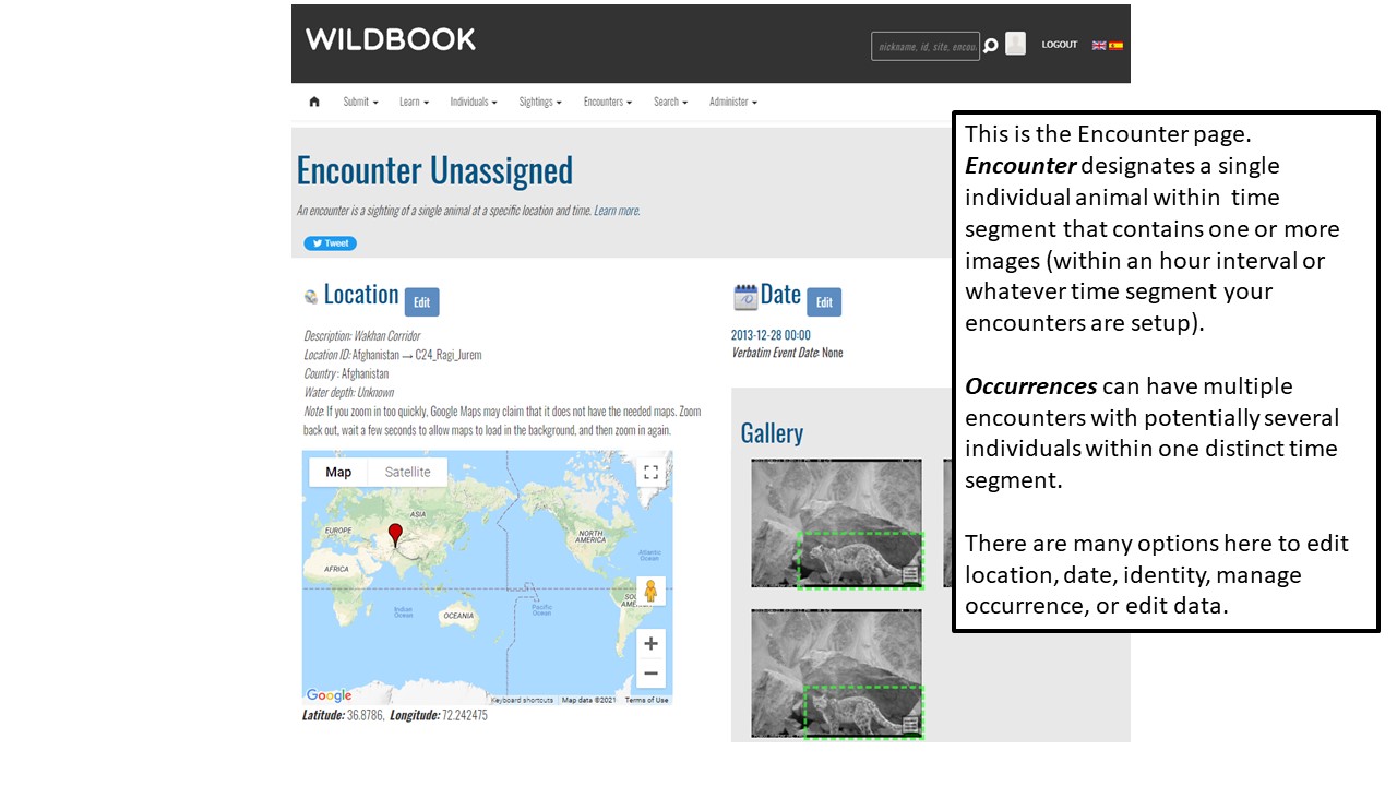
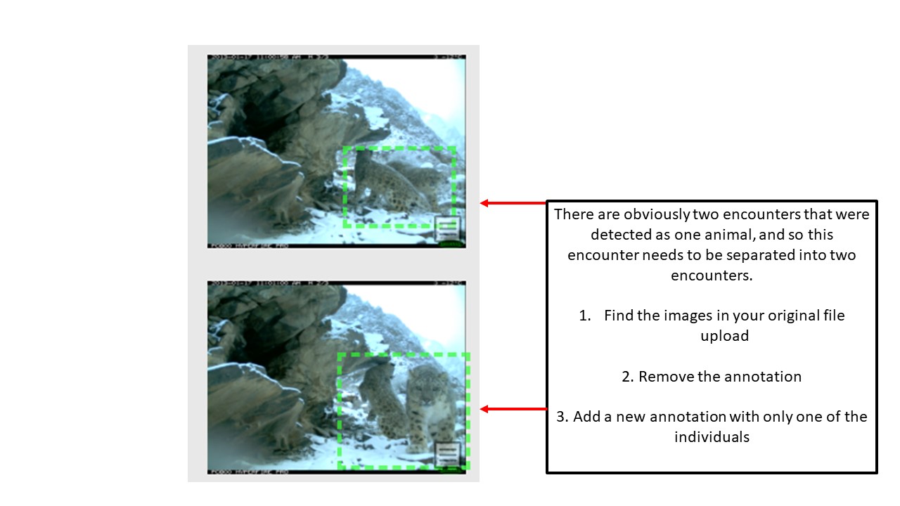
- An occurrence is a set of images that are normally associated to one time span, like an hour where the same animals were passing in front of the camera.
- An encounter is a sighting of one animal within that time span. It is possible to encounter more than one individual over the course of an hour, although that hour is still called an occurrence and the single animals within are called the encounter.
For animal encounter data, it depends on the length of time you would like to subset the data. For the purposes of this lesson, we will group the data into occurences by hour. Each row of our whiskerbook dataframe will represent an encounter. Although at this early stage, we likely do not know if there are multiple individuals within the hour. To start, we will break up our data into hourly subsets and work with that. If possible, going through the data carefully to understand where there are multiple individuals and sorting it out early can be an advantage. It will keep the data clean and avoid problems later. Although, in the Whiskerbook program it is fairly easy to delete images from one encounter and create a new encounter with images from the second individual. It is up to you how you will deal with this issue. However time consuming it may be to sort the data by individual early on may save time later.
Here we use the dplyr functions for group_by to group the camera trap photos by location ID of the camera station, and the year, month, day, and hour. Then, after they are grouped, we simply sequentially number each individual photo and assign it to which group it is in.
The mutate function within dplyr allows us to create a new row of data based on some function or command, in this case, we will use the cur_group_id() to ID each of the rows according to which group they are in. The group will then denote the hourly intervals, which are our occurrences.
  Whiskerbook_template<-Whiskerbook_template%>%
  group_by(Encounter.locationID, Encounter.year, Encounter.month, Encounter.day,Encounter.hour)%>%
  mutate(Encounter.occurrenceID = cur_group_id())
Challenge: group_by function
Answer the following questions:
- What happens when you group by different columns? Experiment with grouping by fewer or more columns to see the result. What happens to the group_ids?
Next, we have to sequentially number each of the images within that group or “occurrence” to create the Encounter.mediaAsset information that Whiskerbook needs to have. Now, within each group we are numbering each photo within that group. There may be 10 photos in an occurrence so they would be numbered 1-10, or there may be 40 photos within the occurrence, so we name those 1-40. Thankfully, dplyr has all of the necessary functions to allow us to name the photos within each group.
Whiskerbook_template<-Whiskerbook_template%>%
  group_by(Encounter.occurrenceID)%>%
  mutate(Encounter.mediaAsset = 1:n())
The image numbers we just created are actually going to become column names, and so we need to add the characters “Encounter.mediaAsset” before these numbers. To do this, we can use the paste function to paste together our character string and the number we generated.
Whiskerbook_template$Encounter.mediaAsset<-paste("Encounter.mediaAsset", Whiskerbook_template$Encounter.mediaAsset, sep="_")
Now, we will cast the Encounter.mediaAsset column out. Which means we will take one column of data, and generate numerous columns. Check to see the result of this if you are unsure what just happened.
We are calling this new template Whiskerbook_template2
library(reshape2)
Whiskerbook_template2<-dcast(Whiskerbook_template,Encounter.occurrenceID~Encounter.mediaAsset, value.var ="Encounter.mediaAssetX")
As you can see, the columns are not sorted sequentially, so we need to sort them by ascending order. The str_sort function in the stringr can sort the columns.
library(stringr)
Whiskerbook_template2_cols<-str_sort(colnames(Whiskerbook_template2), numeric = TRUE)
Whiskerbook_template2<-Whiskerbook_template2[,Whiskerbook_template2_cols]
Next, we have to actually rename all of the Encounter.mediaAsset columns starting with 0. They start with 1 now because the dply package requires we number starting with 1 not 0. It’s a bit of a glitch for us, but we can fix this.
First, we can create a vector of numbers for the number of occurrences that we have. Then, we add the characters “Encounter.mediaAsset” to these numbers. Then we add one more column name for the “Encounter.occurrenceID” that is already in our dataframe. Now we have a vector of character strings that will be our new column names.
Now, we can simply rename our dataframe columns using the new names we have created.
#the columns have to be renamed from 0 so we subtract one from the length
#the final column is the Encounter.occurrenceID column so we subtract one
col_vec<-0:(length(Whiskerbook_template2)-2)
col_vec<-paste("Encounter.mediaAsset",col_vec, sep="")
Media_assets<-c(col_vec, "Encounter.occurrenceID")
names(Whiskerbook_template2)<-Media_assets
The next thing we need to do is clean up our original Whiskerbook template so that we can merge these new cast Encounter.mediaAsset data.
In the original template, now, we have all the filenames in an Encounter.mediaAssetX column, and we need to remove that. That was there originally before we went through the trouble of reorganizing it.
Finally, we can remove the Encounter.mediaAsset column, which contained the numbers assigned to the individual images, we will also remove the final column for the original numbered images within the hourly subsets.
Whiskerbook_template<-Whiskerbook_template[,-1]
Whiskerbook_template <-Whiskerbook_template[,-ncol(Whiskerbook_template)]
Then, we will take only the unique records within this template.
Whiskerbook_template<-unique(Whiskerbook_template)
Then, remove all of the columns which are filled with only NA values. We do not need these columns if they have no information and the file can still be uploaded.
Whiskerbook_template<-Whiskerbook_template[,colSums(is.na(Whiskerbook_template))<nrow(Whiskerbook_template)]
Now our original Whiskerbook template is formatted so we can merge the Whiskerbook_template2 with our cast Encounter.mediaAsset filenames to it. To do this, we can merge the templates together using the merge function, and then select only the unique rows.
Whiskerbook<-merge(Whiskerbook_template,Whiskerbook_template2, by="Encounter.occurrenceID", all.x=FALSE, all.y=TRUE)
Whiskerbook<-unique(Whiskerbook)
Finally, we are left with a template with our occurrences with the filenames cast into rows. We will write this to file for batch import into Whiskerbook.
write.csv(Whiskerbook, "Whiskerbook.csv")
Key Points
Whiskerbook takes a specific format for data upload
Casting the file names into long format for Encounter.mediaAsset
Wildbook Data Portal Tutorial
Overview
Teaching: 60 min
Exercises: 30 minQuestions
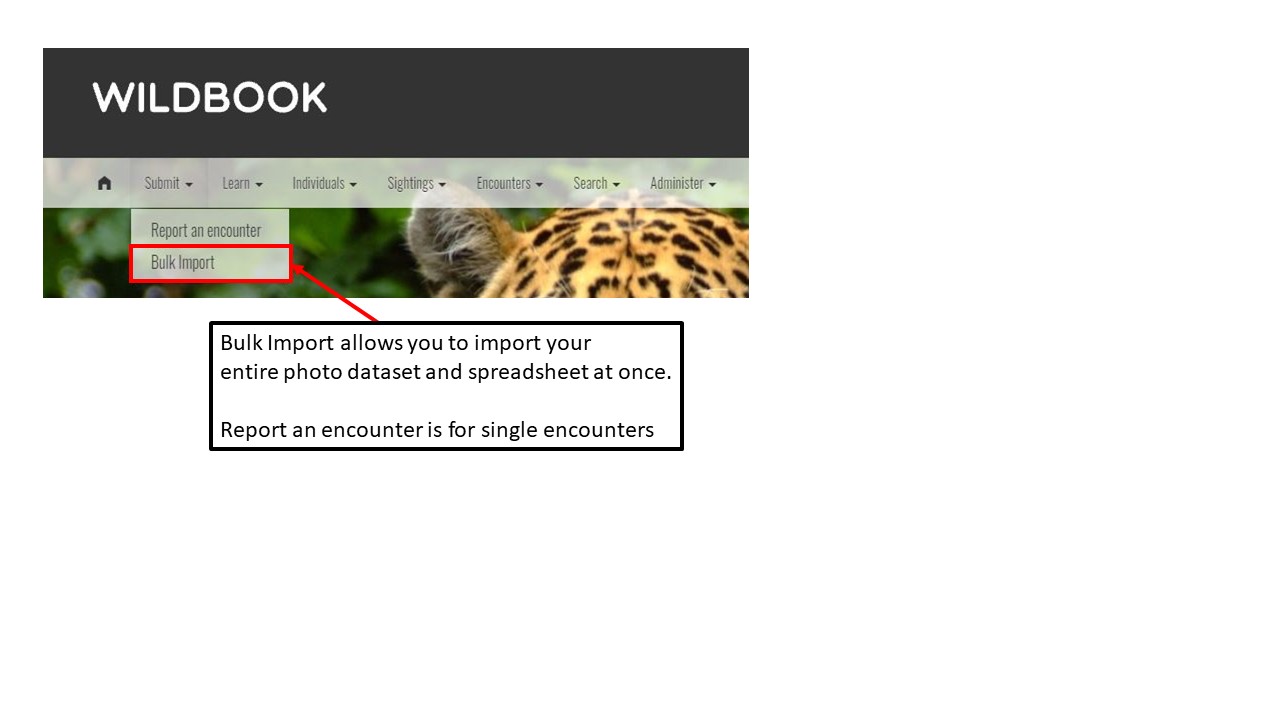
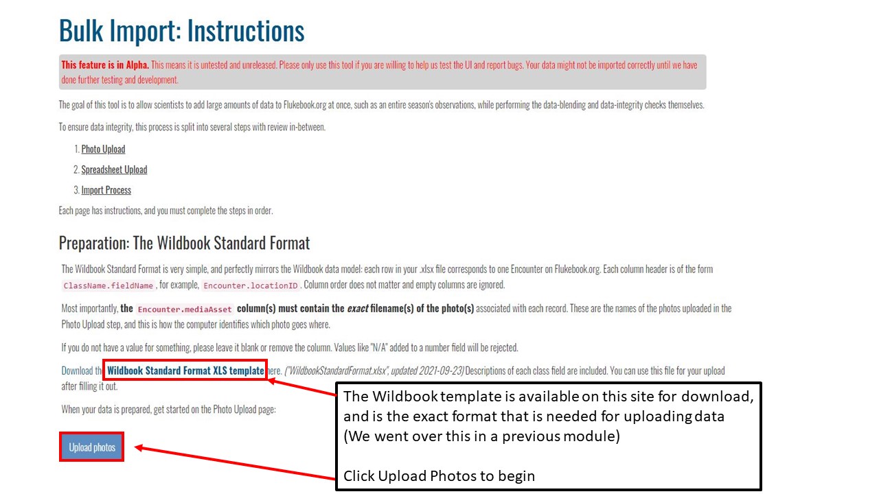
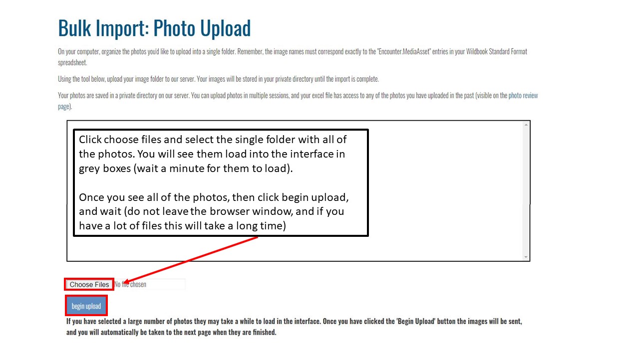
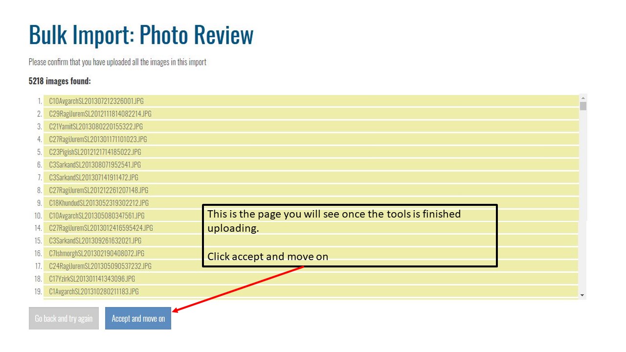
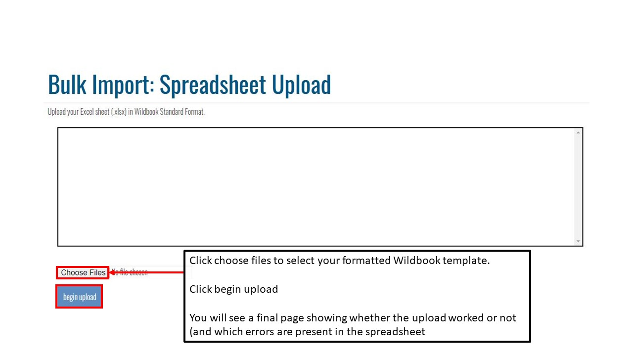
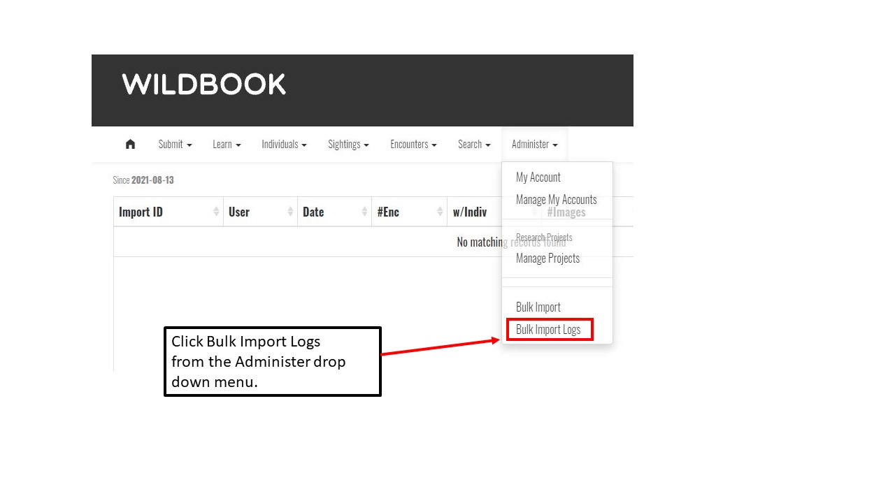
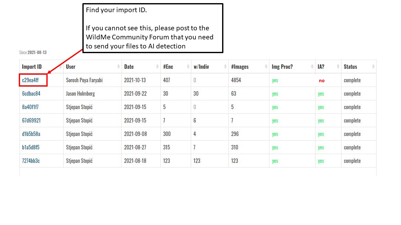
How do I bulk import data into the interface?
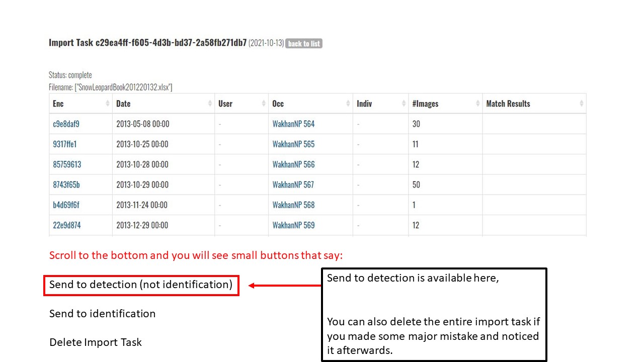
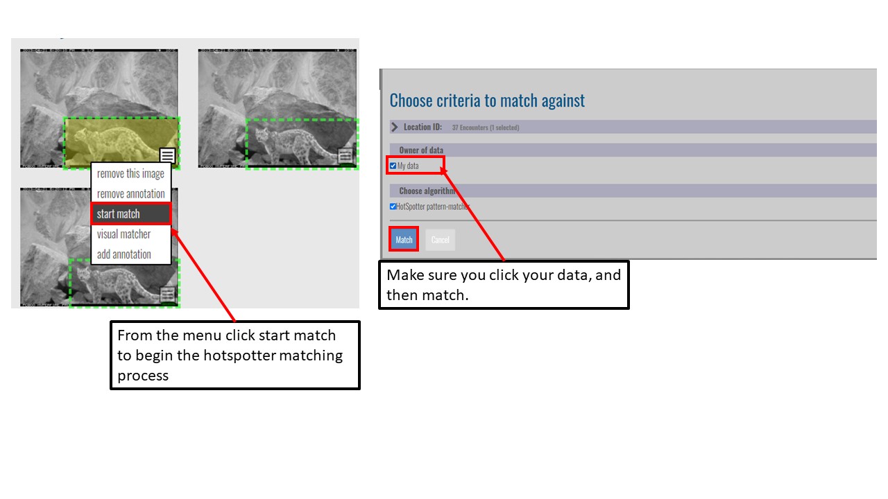
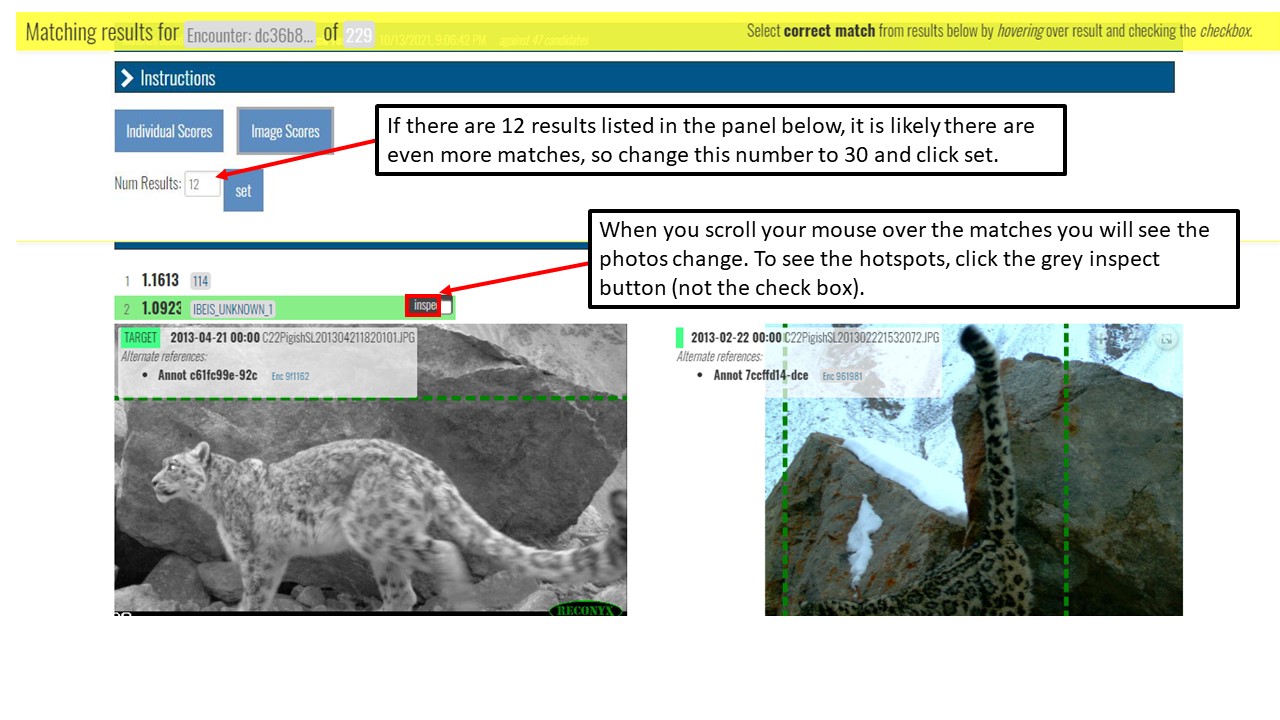
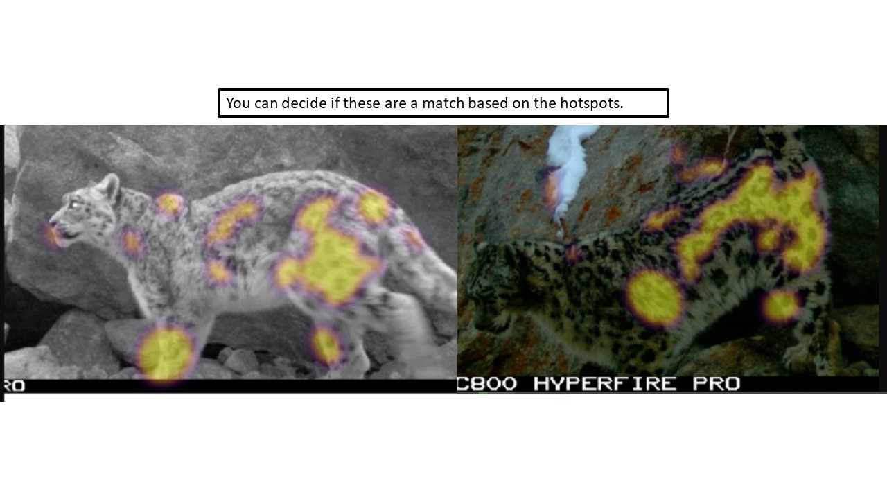
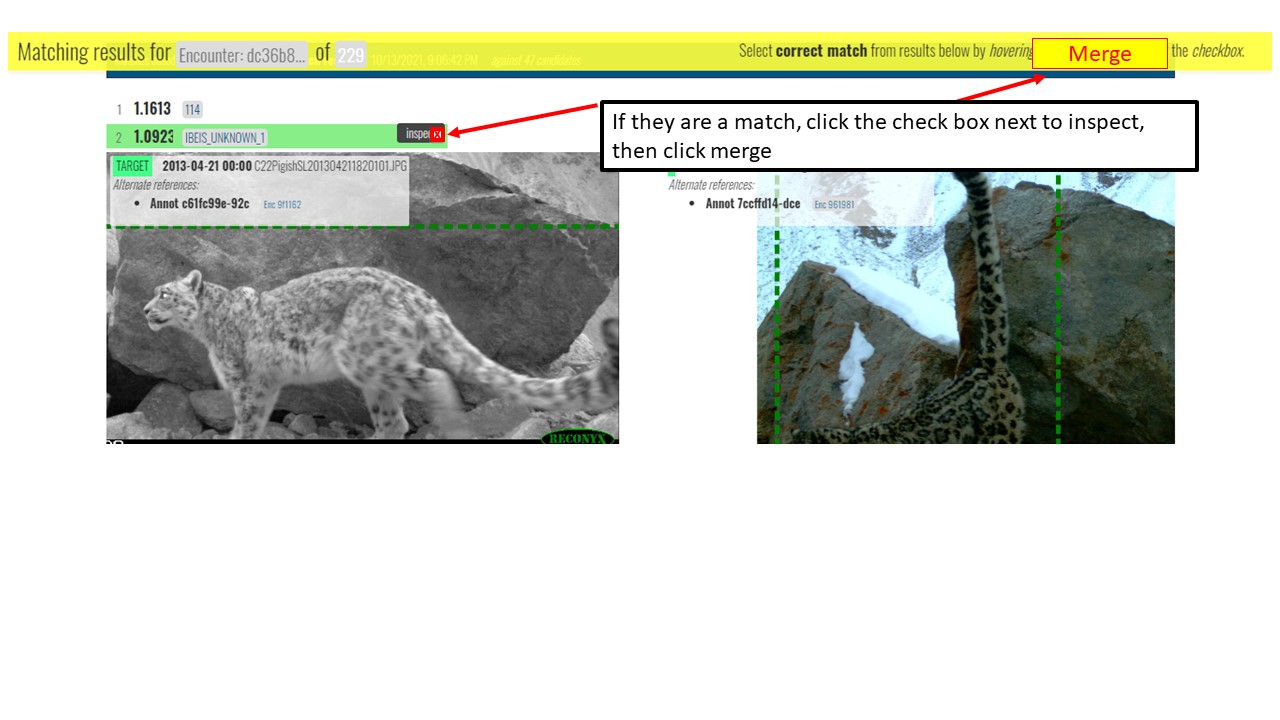
How can I run hotspotter on my images?
How do I use the visual matcher?
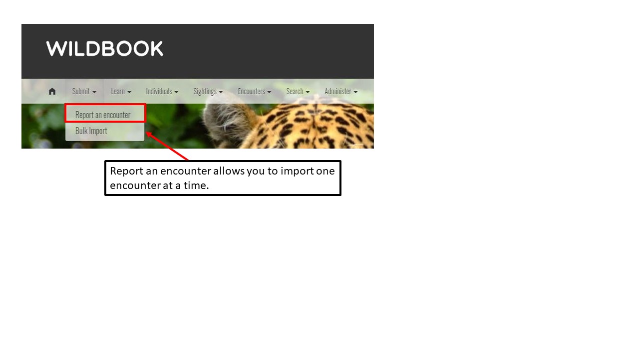
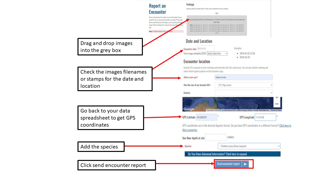
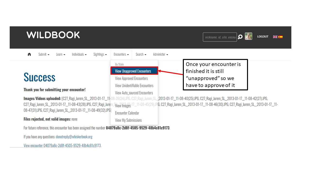
How can I report an encounter?
Objectives
Learn how to use the Wildbook for individual identification
Here the instructor will show you how to use the Whiskerbook interface using an account already setup. You will also have access to this account. Please do not change or delete anything in this instructional account. It mainly serves as to orient you to using the platform and seeing how it works. This webpage are notes as reference for future dates when you come back to using the Whiskerbook portal, in case you forgot something.
When you are ready to upload an your data formally, please email me @ evebohnett@yahoo.com as I am a volunteer Project Director for the Whiskerbook and first point of contact for any support issues you may have.
 #########################################################
 #########################################################
 #########################################################
 #########################################################
 #########################################################
 #########################################################
 #########################################################
 #########################################################
 #########################################################
 #########################################################
 #########################################################
 #########################################################
 #########################################################
 #########################################################
 #########################################################
 #########################################################
 #########################################################
 #########################################################
 #########################################################
 #########################################################
 #########################################################
 #########################################################
 #########################################################
 #########################################################
 #########################################################
 #########################################################
 #########################################################
 #########################################################
 #########################################################
 #########################################################
 #########################################################
 #########################################################
 #########################################################
 #########################################################
 #########################################################
Key Points
Upload data into the Wildbook
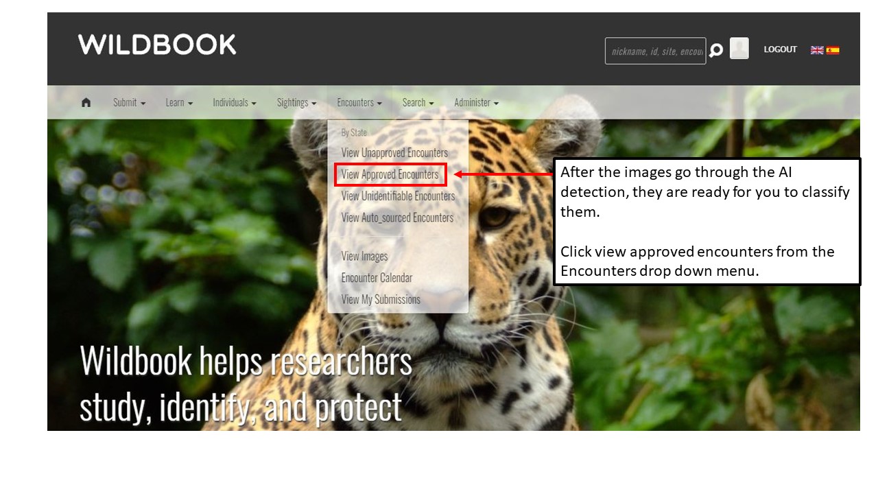
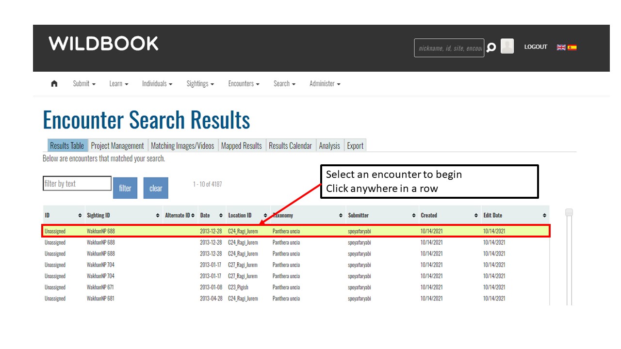
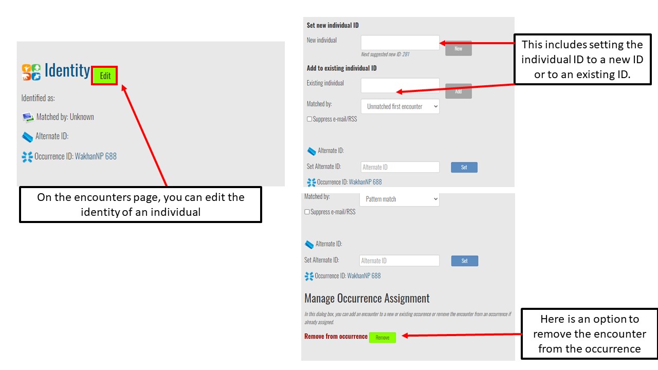
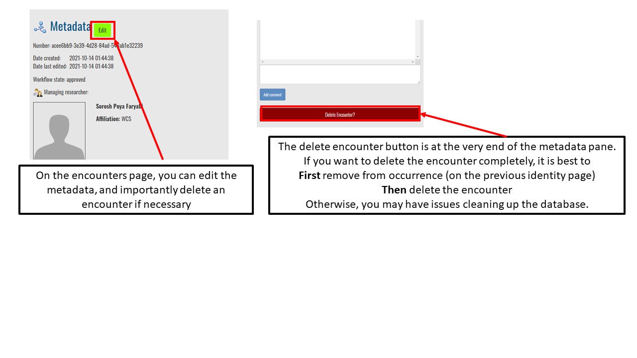
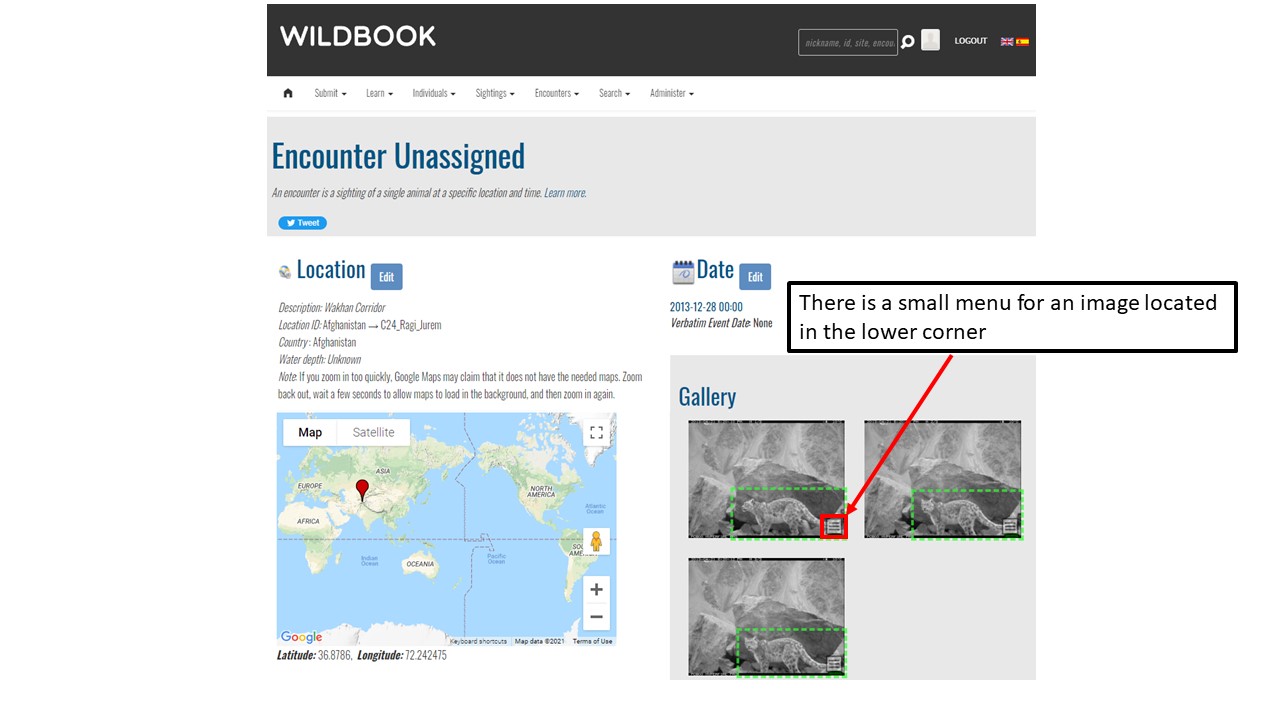
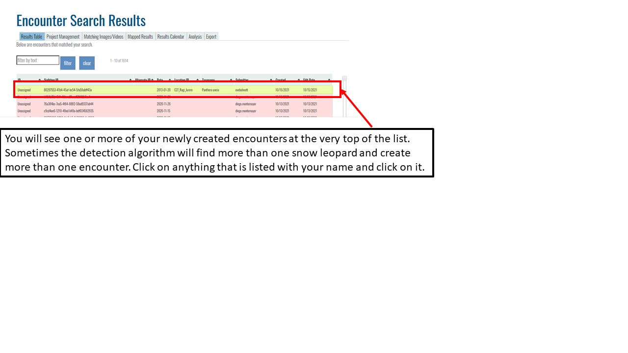
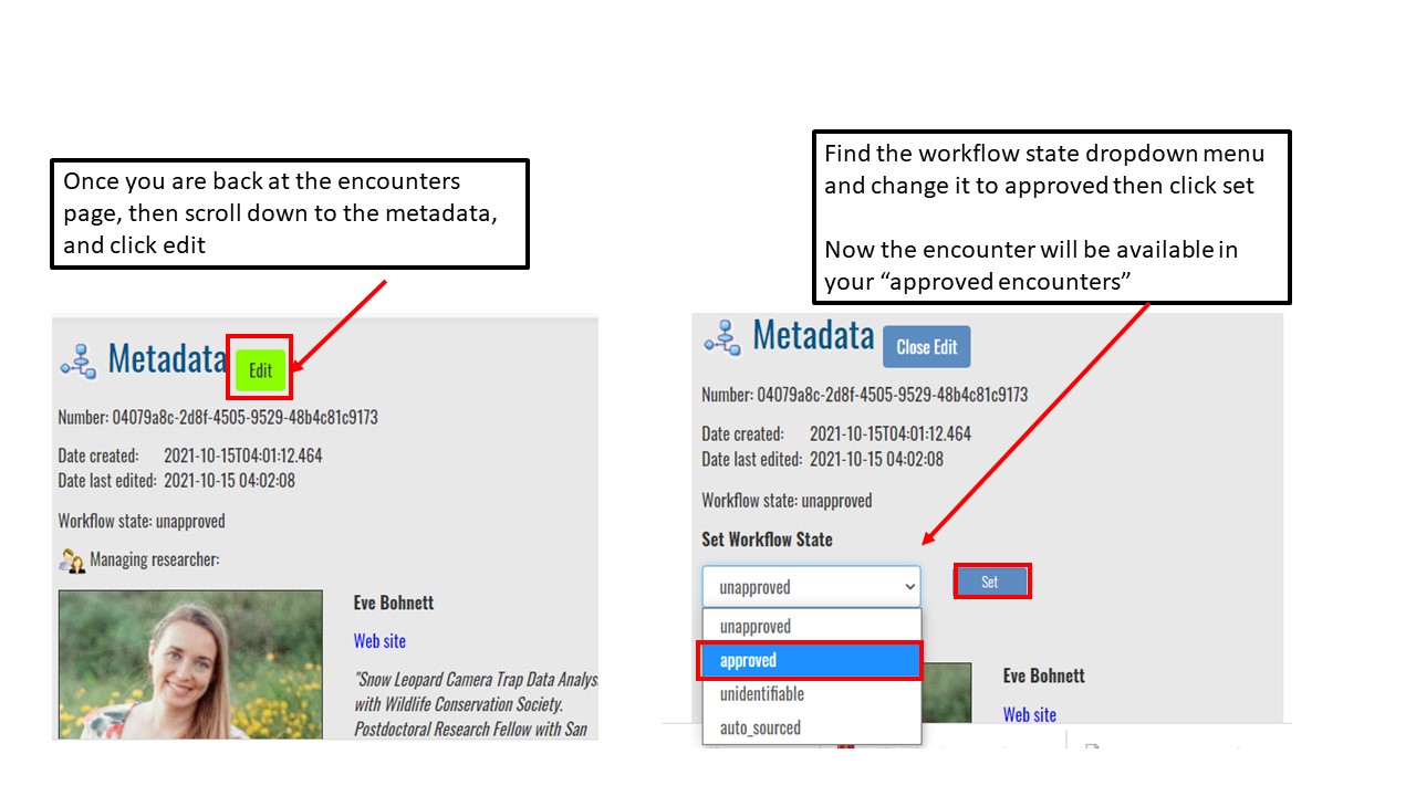
Understand encounters and how to navigate the encounters page
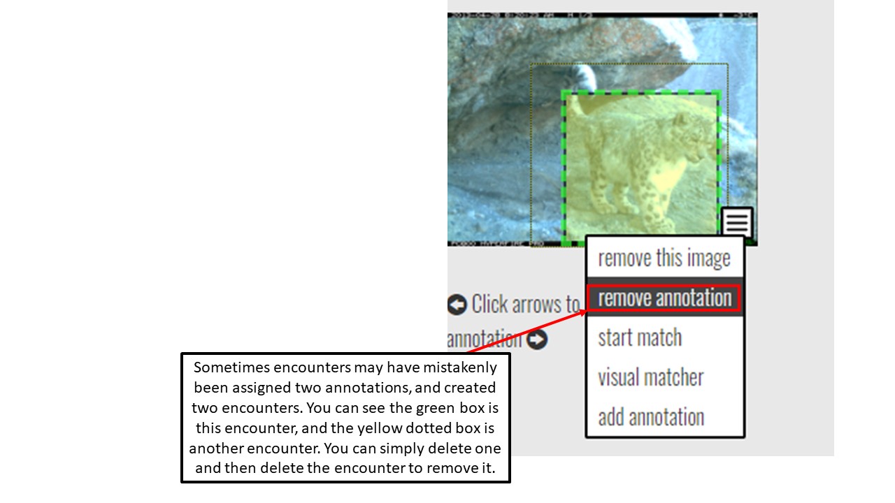
Effectively delete encounters
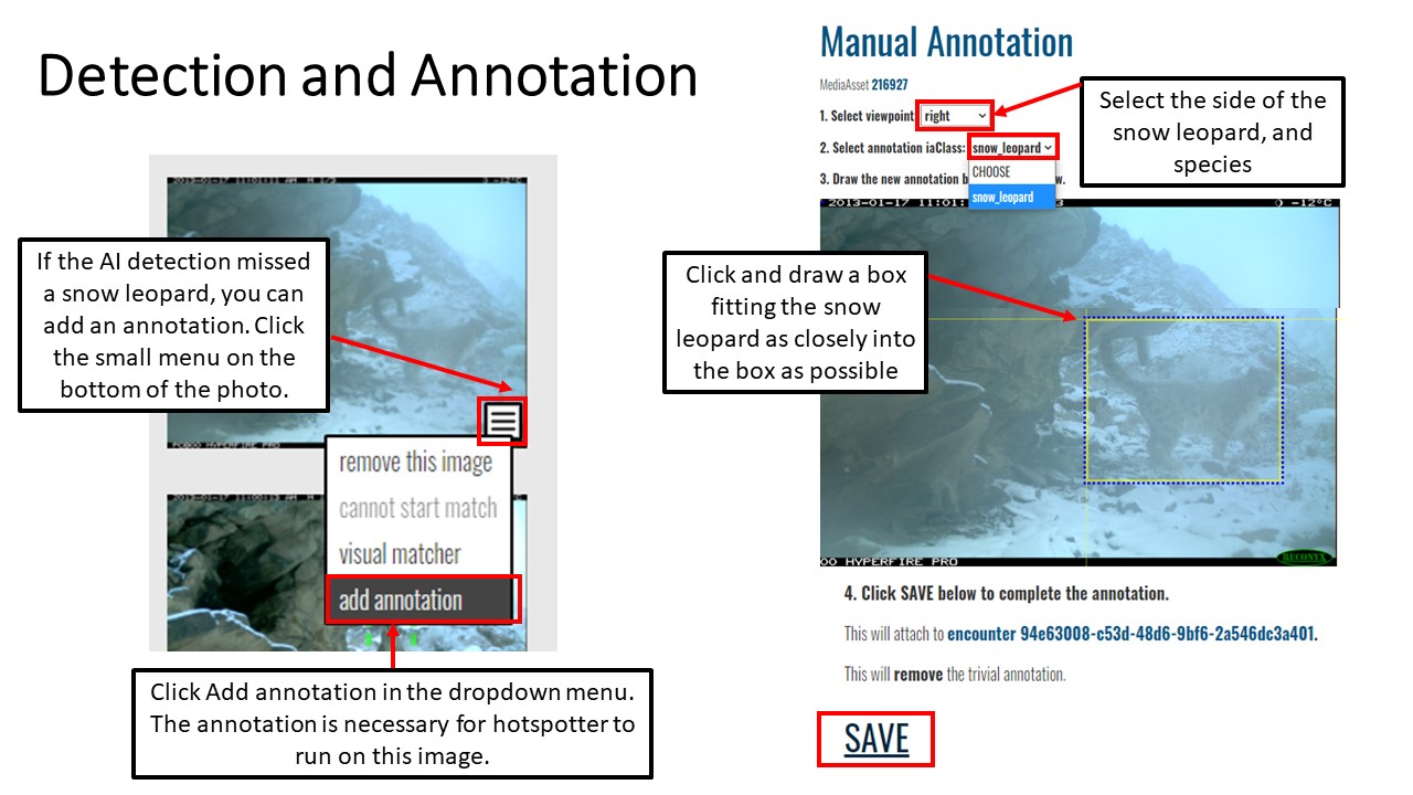
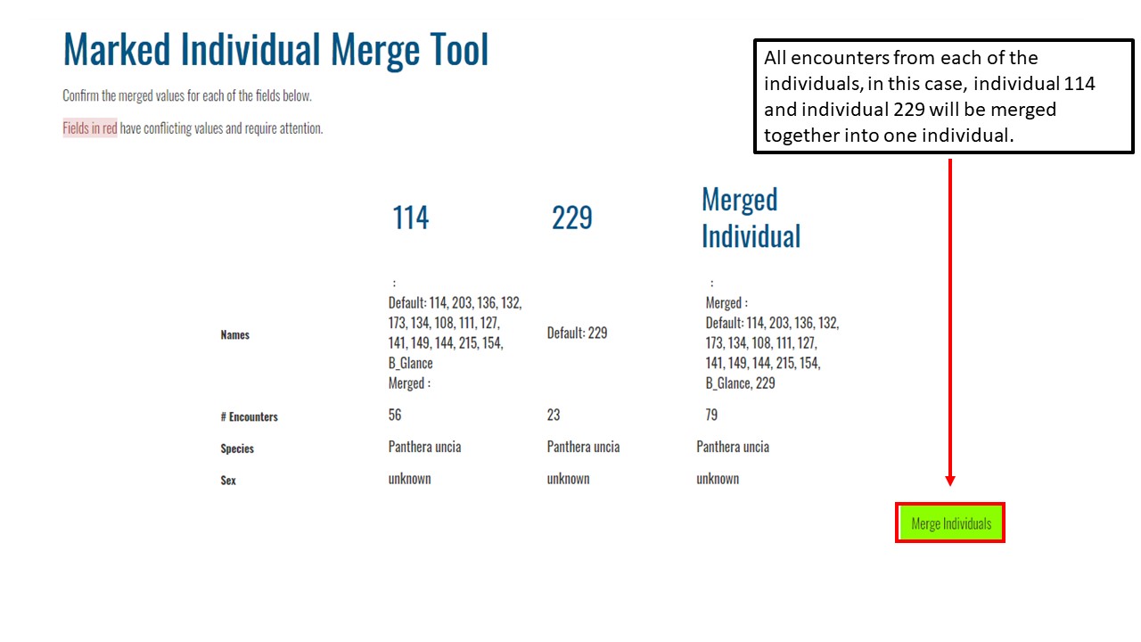
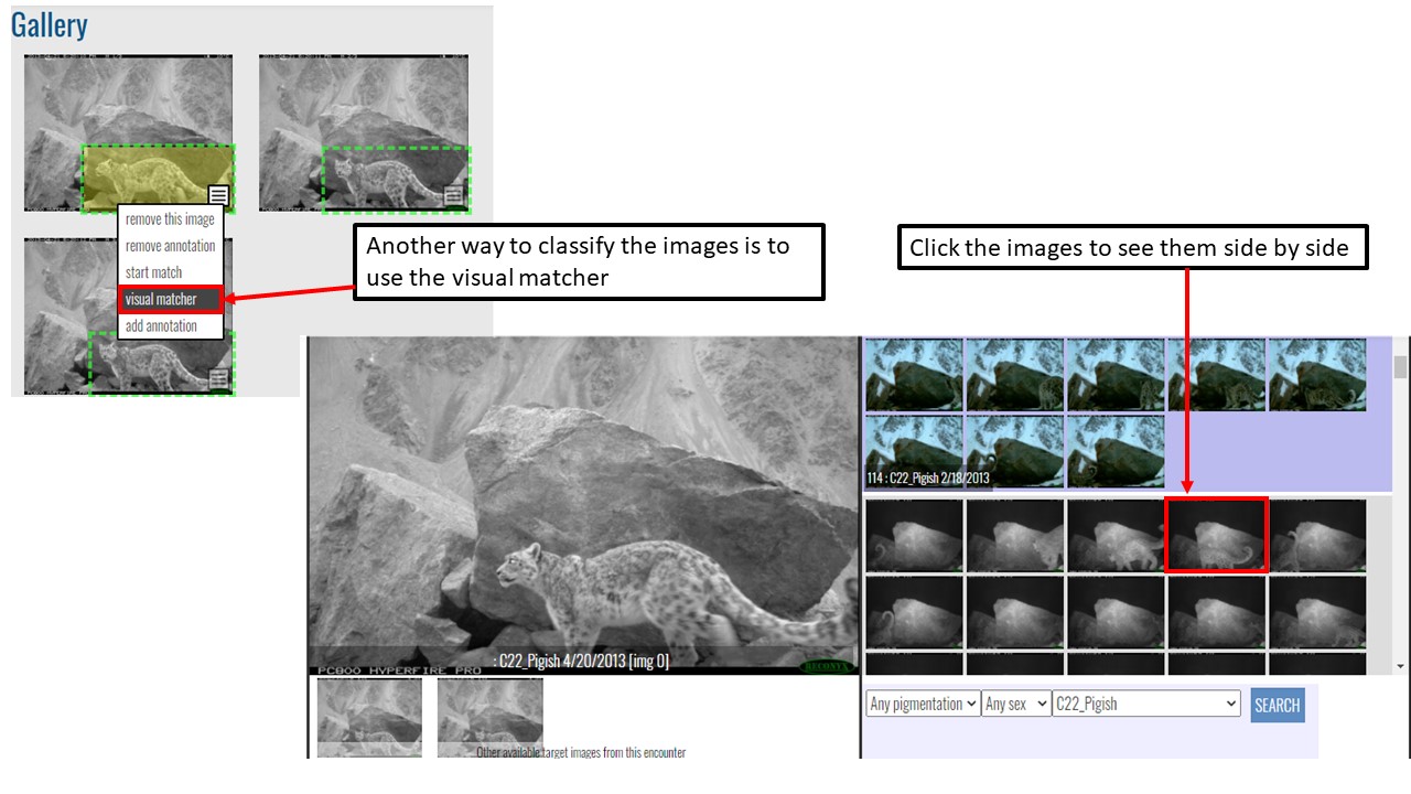
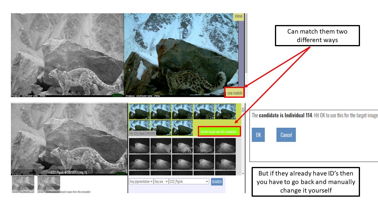
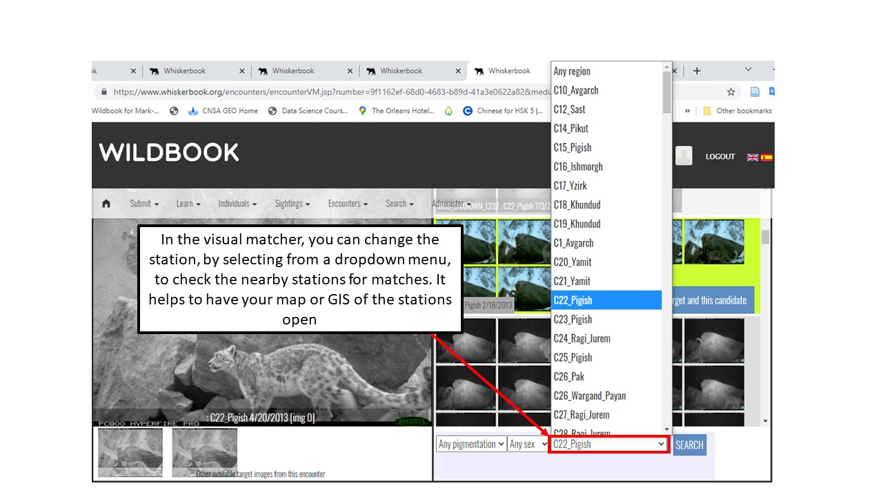
Use Hotspotter and Visual Matcher for individual identification
Report an encounter
Whiskerbook Post-Export
Overview
Teaching: 60 min
Exercises: 30 minQuestions
How to manipulate data for descriptive information
How can we organize data using dplyr?
How can we organize data for input into oSCR?
Objectives
Perform data wrangling and manipulation of camera trap data
Create the necessary formats for data to be input into oSCR
Here are a few of the packages we will be using in this session. Let’s load them first thing.
library(sf)
library(dplyr)
library(stringr)
We will import the Whiskerbook file that was exported from the website interface. We are finished with the individual identification tasks. These are the raw data that were downloaded and then annotated with labels for whether the photo capture was high or low quality, and if the encounter showed the left, right, or both sides of the animal. You may choose to label head and tail only images as well. These labels had to be placed manually and are at the discretion of the researcher.
Wildbook<-read.csv("Whiskerbook_export.csv")
Let’s do some quick data crunching to find out how many individuals we have in our dataset.
#To find the number of individuals that are in the dataset
IndividualsCount<-Wildbook%>%
  count(Name0.value, sort = TRUE)

IndividualsCount2<-IndividualsCount%>%
  count(n, sort = TRUE)

Individuals<-unique(Wildbook$Name0.value)
Next, we can check to see how many encounters we had on each side of the animal and whether they were low or high quality images.
#To find the number of encounters on each side of the animal and quality
Sides<-Wildbook%>%
  group_by(Side, Quality)%>%
  count(sort = TRUE)
Challenge: Individuals and Sides
Answer the following questions:
How many individuals do we have that were detected once? How many individuals were detected more than once?
What if we wanted to find out how many individuals were detected in each of the years 2012 and 2013?
Solution
- All of the individuals were detected more than once. There were two individuals detected twice.
1.
Individuals_Date<-Wildbook%>%
  group_by(Encounter.year)%>%
  count(Name0.value, sort = TRUE)
Individuals_Date_Totals<-Individuals_Date%>%
   group_by(Encounter.year)%>%
   count()
In this next part, we are beginning our construction of a data matrix that we can use for Spatial Capture recapture. The oSCR package requires a certain format for the data, and to get it into the format that oSCR wants, we have to change a few things.
First, we would like to reconstruct a full date object. Remember our data were previously parsed into year, month and day columns, and now we want a full date again.
#To format dates into a date object we have to combine the month, day and year columns together
Wildbook$date_Time<-paste(Wildbook$Encounter.year, Wildbook$Encounter.month, sep="-")
Wildbook$date_Time<-paste(Wildbook$date_Time, Wildbook$Encounter.day, sep="-")
dateFormat<-"%Y-%m-%d"
Wildbook$date_Time<-as.Date(Wildbook$date_Time,format= dateFormat)
Next, we will reload the metadata file that we had used previously with our GPS and camera functionality information.
Metadata<-read.csv("Metadata_CT_2012_2.csv")

#check whether the location names are exactly the same in the Wildbook download and the metadata
setdiff(Wildbook$Encounter.locationID, Metadata$Trap.site)
Challenge how to fix these missed entries? From a previous lesson we learned how to manipulate the data to have matching file names.
Metadata$Trap.site<-str_replace(Metadata$Trap.site,"C18_Khandud","C18_Khundud")
Metadata$Trap.site<-str_replace(Metadata$Trap.site
,"C26_Wargand Payan","C26_Wargand_Payan")
Metadata$Trap.site<-str_replace(Metadata$Trap.site
,"C27_Ragi Jurum","C27_Ragi_Jurem")
Metadata$Trap.site<-str_replace(Metadata$Trap.site
,"C30_Wargand Payan","C30_Wargand_Payan")
Metadata$Trap.site<-str_replace(Metadata$Trap.site
,"C32_Wargand Bala","C32_Wargand_Bala")
Metadata$Trap.site<-str_replace(Metadata$Trap.site
,"C45_Avgarch" ,"C45_Avgach")
Metadata$Trap.site<-str_replace(Metadata$Trap.site
,"C5_Ishmorg" ,"C5_Ishmorgh")
Check again whether the names are all exactly the same by using setdiff.
setdiff(Wildbook$Encounter.locationID, Metadata$Trap.site)
Then, we can merge the metadata into our Wildbook download.
Wildbook2<-merge(Metadata, Wildbook, by="Trap.site", by.y="Encounter.locationID", all=TRUE)
Our metadata has more locations then we actually need for these data. So, we can subset the dataframe to include only those locations that are actually in the Wildbook.
Metadata<-Metadata[which(Metadata$Trap.site %in% Wildbook$Encounter.locationID),]
Let’s save our subset Metadata for later.
write.csv(Metadata, "Metadata.csv")
Now, we only will need certain columns of our Wildbook data. We can easily subset these needed columns and rename them.
We will also subset the GPS coordinates for our locations into a separate object called Wildbook_points_coords.
Wildbook_points<-Wildbook2[,c("Name0.value","Encounter.decimalLongitude", "Encounter.decimalLatitude", "Trap.site", "date_Time", "Side","Quality", "Juvenilles") ]

#rename the columns to more recognizable names
colnames(Wildbook_points)<-c("Marked.Individual", "Latitude", "Longitude", "Location.ID","date_Time" ,"Side", "Quality","Juvenilles")

#subset the coordinates.
Wildbook_points_coords<-unique(Wildbook_points[,c(2,3,4)])
Now, we will need to transform the lat/long coordinates in the Wildbook back to UTM.
library(sf)
wgs84_crs = "+init=EPSG:4326"
UTM_crs = "+init=EPSG:32643"

Wildbook_points_coords<-Wildbook_points_coords[complete.cases(Wildbook_points_coords),]

Wildbook_pts_latlong<-st_as_sf(Wildbook_points_coords, coords = c("Latitude","Longitude"), crs = wgs84_crs)

#We can plot the coordinates to make sure they are correctly configured.

plot(Wildbook_pts_latlong[1])
Then we can transform the points back into UTM.
Wildbook_pts_utm<-st_transform(Wildbook_pts_latlong, crs = UTM_crs)
#extract the UTM coordinates
Wildbook_pts_utm_df<- st_coordinates(Wildbook_pts_utm)

#add the UTM coordinates bto the Wildbook_points_coords object
Wildbook_points_coords<-cbind(Wildbook_points_coords, Wildbook_pts_utm_df)

#merge the coordinates back to the Wildbook dataframe.
Wildbook_points<-merge(Wildbook_points_coords, Wildbook_points, by=c("Location.ID", "Latitude", "Longitude"))
A few more pieces of data are needed, mainly the Session information and the Occassion. In our case, for modeling purposes this time, these will initially be set to 1. We will change these later.
Wildbook_points$Session<-1
Wildbook_points$Occassion<-1
Wildbook_points$species = "Snow Leopard"
Next, we will use the camTrapR package to create a matrix of camera operations.
We will use our metadata with the dates the cameras were intially deployed and then taken down.
The package can also accommodate any problems with the cameras during the session, for example, if one camera had a technical issue and had to be taken down and replaced a month later, that would be included in separate columns for problems. In our case, we do not have any data about problems, so we set this parameter to FALSE.
The result of this function is a site x dates matrix of which days the cameras were operational.
dateormat <- "%Y-%m-%d"

Metadata$Start<-as.Date(Metadata$Start)
Metadata$End<-as.Date(Metadata$End)

# alternatively, use "dmy" (requires package "lubridate")
library(camtrapR)
camop_problem <- cameraOperation(CTtable      = Metadata,
                                 stationCol   = "Trap.site",
                                 setupCol     = "Start",
                                 retrievalCol = "End",
                                 hasProblems  = FALSE,
                                 dateFormat   = dateFormat)
The oSCR program requires the data come in a specific format to run the models. Here we will wrangle the data into the proper format. In our case, we will simply subset our dataframe into the necssary columns.
The first dataframe we want to create is a record of the individual occurrences with the dates, trap site, side and quality.
#create the subset dataframe
edf<-Wildbook_points[,c("Marked.Individual", "date_Time","Location.ID","Side","Quality", "Juvenilles")]

#convert the dates to date format
edf$date_Time<-as.Date(edf$date_Time)
We will also create a dataframe based on site and GPS coordinates. Here, we want to use the data in UTM coordinates.
tdf<-unique(Wildbook_points_coords[,c("Location.ID","X", "Y")])
Now, we will create a merged dataframe with all elements both the dataframe with the GPS coordinates and the dataframe with the information for the individual IDs.
We will save this file for the next lesson.
edf_tdf<-merge(edf,tdf,by="Location.ID")
Eliminate any duplicated values, this table containes duplicates from the way whiskerbook can create multiple encounters from the same occurrence, so the data are a bit messy.
write.csv(edf_tdf, "edf_tdf.csv")
The oSCR program requires we append the camera operation matrix to the tdf table with the GPS coordinates.
In order to make this as clear as possible, we will rename our camera operations matrix with numbers for each date, instead of the dates themselves.
#create dataframe objects for the camera operations matrix and the detections.
camop_problem<-as.data.frame(camop_problem)
detectionDays<-as.data.frame(colnames(camop_problem))

#create a sequential numeric vector for the number of detection dates
detectionDays$Occasion<-1:nrow(detectionDays)

#rename the columns
colnames(detectionDays)<-c("Dates","Occasion")

#rename the columns with the numeric vector
colnames(camop_problem)<-detectionDays$Occasion

#make a new column of the trap site names so we can merge the dataframes
camop_problem$Location.ID<-rownames(camop_problem)
Next, we will check whether the locations in the GPS coordinates columns exactly match the camera operability matrix.
setdiff(tdf$Location.ID, camop_problem$Location.ID)
Next, we will check whether the locations in the tdf dataframe with the GPS coordinates columns exactly match the edf dataframe about the individuals.
setdiff(tdf$Location.ID, edf$Location.ID)
Now we can merge our camera operability matrix to our tdf dataframe with the camera operability matrix.
#merge the GPS coordinates table with the camera operations matrix
tdf<-merge(tdf, camop_problem, by="Location.ID", all=TRUE)

#remove the column with the trap names from the camera operations matrix
camop_problem<-camop_problem[,-ncol(camop_problem)]
In our edf dataframe about the individuals, then we need to convert our individual names to sequential numbers for clarity.
#convert the individual ID's and locations to sequential numbers for clarity.
edf$ID<-as.integer(as.factor(edf$Marked.Individual))
Check again to make sure the names of the Location.ID columns match.
setdiff(edf$Location.ID, tdf$Location.ID)
setdiff(tdf$Location.ID, edf$Location.ID)
Write the files to csv so we can use them later.
write.csv(edf, "edf.csv")
write.csv(tdf, "tdf.csv")
Challenge: Camera Operability Matrix
Answer the following questions:
- How do we format our data if our camera traps had an issue and were not running for several weeks?
Solution
The cameraOperation matrix has a field called hasProblems that would be set equal to TRUE. The fields in the CTtable would be changed to include fields “Problem_from” and “Problem_to”
Key Points
Use dplyr to get basic descriptive information about the number of individuals
organize encounters and stations in the correct format for oSCR
Whiskerbook Data Manipulation
Overview
Teaching: 60 min
Exercises: 30 minQuestions
How to manipulate data for descriptive information
Objectives
Perform data wrangling and manipulation
Sort only high quality data
Divide data into left only and right only
Initially, we will load the dplyr library and the edf_tdf.csv that we had produced in an earlier lesson.
edf_tdf<-read.csv("edf_tdf.csv")
We had previously manually labeled our encounters with information about Juvenilles.
Lets check this information by looking at the dataframe with ONLY Juvenilles.
#subset the dataframe for records containing juvenilles. These are the
edf_tdf_J<-edf_tdf[which(edf_tdf$Juvenilles=="J"),]
Now, we want to subset only the unique juvenilles from our dataframe based on the individual ID and the date_time signature. We do not want to include more than one encounter from each day. For our purposes, we only need one per day.
We can check the unique individual ID of the juvenilles to find out how many we had encountered during our study.
#subset the dataframe to identify unique individuals
edf_tdf_J<-unique(edf_tdf_J[,c("Marked.Individual","date_Time")])

#pull the indiviudal ID out
edf_tdf_J_ID<-unique(as.character(edf_tdf_J$Marked.Individual))
Lets remove the Juvenilles from our dataframe, since we won’t need them for our analysis or our descriptions.
In our analysis, we will not include juvenilles for estimates of density or abundance.
#Remove juvenilles from the dataframe
edf_tdf<-edf_tdf[-which(edf_tdf$Juvenilles=="J"),]
Subset the data by distinct fields, since the encounter data can include several encounters from one day. . For this, we will use dplyr to subset based on distinct ID, date_time, Side, and location ID. That way, we have a complete case of records and nothing extra.
#get unique records by several fields using distinct
edf_tdf_d<-edf_tdf %>% distinct(Marked.Individual, date_Time, Side, Location.ID, .keep_all = TRUE)
Next we can create some dataframes of high quality and low quality encounters.
edf_tdf_high<-edf_tdf_d[which(edf_tdf_d$Quality=="H"),]
edf_tdf_low<-edf_tdf_d[which(edf_tdf_d$Quality %in% c("L","M")),]
Now we will do some basic descriptions of the left and right hand sides and determine which individuals have left sides and right sides, or only one or the other.
ID_left_right<-edf_tdf_high%>%
  group_by(Marked.Individual, Side)%>%
  count()
Let’s subset the data that are annotated with either left and right.
ID_left_right_sub<-ID_left_right[which(ID_left_right$Side %in% c("L", "R")),]
Lets see how many individuals have only the left side or right side by counting the records grouped by ID.
ID_left_right_sub_final<-ID_left_right_sub%>%
  group_by(Marked.Individual)%>%
  count()
From this,we can find the records which are left only or right only individuals.
OneSided<-ID_left_right_sub_final[which(ID_left_right_sub_final$n==1),]
TwoSided<-ID_left_right_sub_final[which(ID_left_right_sub_final$n==2),]
Now we can find which individuals have one side or both sides.
ID_oneOnly<-ID_left_right_sub[which(ID_left_right_sub$Marked.Individual %in% OneSided$Marked.Individual),]
ID_twoSided<-ID_left_right_sub[which(ID_left_right_sub$Marked.Individual %in% TwoSided$Marked.Individual),]
From this we can find the individuals that are one sided and right only or left only.
ID_oneOnly_right<-ID_oneOnly[ID_oneOnly$Side=="R",]
ID_oneOnly_left<-ID_oneOnly[ID_oneOnly$Side=="L",]
Now we can subset the dataframe to remove the records that are right only to create the left only dataframe. Similarly, when we subtract out the left only records, then we have a right only dataframe.
edf_left<-edf_tdf_high[-which(edf_tdf_high$Marked.Individual %in% ID_oneOnly_right$Marked.Individual),]
edf_right<-edf_tdf_high[-which(edf_tdf_high$Marked.Individual %in% ID_oneOnly_left$Marked.Individual),]
Challenge: Camera Operability Matrix
Answer the following questions:
- How many individuals were back only?
  ID_back_final<-ID_left_right%>%
 group_by(Side)%>%
 count()
From this result, we can see that 9 detections were back, and 3 were tail only.
Key Points
Subset left and right only individuals
Subset individuals that have encounters that include both left and right sides
Subset dataframes that include left only and both sides, and right and both sides
Spatial-Capture Recapture Data Preparation
Overview
Teaching: 60 min
Exercises: 30 minQuestions
How to setup single 3 month season oSCR data?
How to setup our oSCR data that exclude areas of high elevation?
What is a buffer mask and how to parameterize it?
Objectives
Perform spatial capture recapture modeling data preparation
Split data into intervals for months
Change working directory and load several packages, including oSCR, raster, dplyr, and camtrapR.
Read in our tdf, edf, and metadata files that we created in the previous lesson.
tdf<-read.csv("tdf.csv", stringsAsFactors = TRUE)
edf<-read.csv("edf.csv", stringsAsFactors = TRUE)
Metadata<-read.csv("Metadata.csv")
There are three raster layers that are suitable for this analysis, including the roughness, topographic position index and elevation. To generate these layers, the elevation was downloaded as an SRTM file, the roughness and topographic position index were calculated using the terrain function in the terrain package in program R.
roughness<-raster("GeospatialData/roughness.tif")
TPI<-raster("GeospatialData/TPI2.tif")
elev<-raster("GeospatialData/elev.tif")
First, we have to change the date formats to be suitable for the dates to be recognized. Right now, they are in character string format.
#specify the format for the dates
dateFormat <- "%Y-%m-%d"

#convert the character strings to date formats
Metadata$Start<-as.Date(Metadata$Start,format= dateFormat)
Metadata$End<-as.Date(Metadata$End, format=dateFormat)
Next, we will use the cameraOperation function in the camtrapR package to generate a site x date matrix for the dates and sites that the cameras were operational. Notice there are several functions that we are not using, although you may for your data. There are options here for setting cameras which have problems for example and were decommissioned for a certain amount of time.
# alternatively, use "dmy" (requires package "lubridate")
camop_problem <- cameraOperation(CTtable      = Metadata,
                                   stationCol   = "Trap.site",
                                   setupCol     = "Start",
                                   retrievalCol = "End",
                                   writecsv     = FALSE,
                                   hasProblems  = FALSE,
                                   dateFormat   = dateFormat)
We need to generate the time intervals for our sessions. In this case, our data is around 4 months, which is too long to assume population closure. We will split our data into 3 month sessions by using the dyplyr package.
#Extract the dates of our surveys that the cameras were operational and create a dataframe
date_cameraop<-as.data.frame(colnames(camop_problem))
#name the column of the new dataframe
colnames(date_cameraop)<-"date_Time"
#convert the characters to dates again
date_cameraop$date_Time<-as.Date(date_cameraop$date_Time)

#Split the sessions into 2 month time intervals using the "cut" function with 3 month breaks.
date_cameraop<-date_cameraop %>%
 mutate(Session_3m = cut(date_Time, breaks= "3 months"))
#convert the sessions to factors, and then to numbers
date_cameraop$Session_3m<-as.factor(date_cameraop$Session_3m)
date_cameraop$Session_3m<-as.numeric(date_cameraop$Session_3m)

#count how many days are within each of the two month intervals
date_cameraop%>%
  group_by(Session_3m)%>%
  count()

#number sequentially the days within each of the grouped 2 month sessions
date_cameraop<-date_cameraop%>%
    group_by(Session_3m)%>%
    mutate(Session_grouped =1:n())
Now, we want to only model a single session, so we will subset our dates to only those in session 1.
#subset the sessions to only one session that we can model
dates_f<-date_cameraop[which(date_cameraop$Session_3m==1),]
#extract out two columns
dates_f_sub<-dates_f[,c("date_Time", "Session_grouped")]
Next, we will subset the dates of session one from the camera operability matrix.
#subset the dates of session 1 from the camera operability matrix.
camop_problem<-camop_problem[,as.character(dates_f$date_Time)]

#remove any rows with only NA values (because those cameras were not setup during session 1!)
camop_problem <- camop_problem[rowSums(is.na(camop_problem)) != ncol(camop_problem), ]

#convert back to a dataframe
camop_problem<-as.data.frame(camop_problem)


#convert NA values to 0 because this will go in our tdf dataframe, which is a list of which cameras were operational.
camop_problem[is.na(camop_problem)]<-0

#change the dates to factors
colnames(camop_problem)<-seq(1,length(camop_problem), by=1)

#create an object with the number of days in the matrix
K=length(camop_problem)
There are further formatting operations that have to be done on the dataframes for the tdf and edf data that we had prepared earlier.
First we start with the tdf dataframe.
#subset our tdf matrix of GPS located station locations by the cameras that were actually operational during our session 1.
tdf2<-tdf[which(tdf$Location.ID %in% rownames(camop_problem)),]
tdf2<-cbind(tdf2[,1:4], camop_problem)
The edf dataframe that can be sorted by the session 1 and we also want to sort only high quality data with no juvenilles (this should be review)
#set the edf dataframe dates
edf$date_Time<-as.Date(edf$date_Time, format= dateFormat)
#merge with the table with the 3m session intervals
edf<-merge(edf, dates_f, by="date_Time")
#convert the sessions to factors, and then to numbers
edf$Session_3m<-as.factor(edf$Session_3m)
edf$Session_3m<-as.numeric(edf$Session_3m)

#subset to Session 1
edf_sub = edf[which(edf$Session_3m==1),]
#subset high quality
edf_high<-edf_sub[which(edf_sub$Quality == "H"),]
#remove juvenilles if there are any
if(sum(edf_high$Juvenilles == "J", na.rm=T)!=0){
  edf_high<-edf_high[-which(edf_high$Juvenilles == "J"),]
}

#merge the dates we had created earlier to get which number from the sequence dates for each of the days in our edf.This column is important for the next step.

edf_high<-edf_high[which(edf_high$Location.ID %in% unique(tdf2$Location.ID)),]
Next we will use the data2oscr function to format the data for our model to an oSCR data object. We can use data2oscr with our edf_high data object, and the tdf2 object. You will see that we can select the columns by name for Session, ID, Occurrence, and Trap.Col. K was the number of days in our survey.
#format the data from our edf_high and tdf2 dataframes and input into the data2oscr function
data <- data2oscr(edf = edf_high,
                  tdf = list(tdf2[,-1]),
                  sess.col = which(colnames(edf_high) %in% "Session_3m"),
                  id.col = which(colnames(edf_high) %in% "Marked.Individual"),
                  occ.col = which(colnames(edf_high) %in% "Session_grouped"),
                  trap.col = which(colnames(edf_high) %in% "Location.ID"),
                  K = K,
                  ntraps = nrow(tdf2))
Load the park boundary shapefile.
library(sf)

#read in the shapefile for the park boundary that we created earlier to reflect the hard boundaries of a river in the north part of the study area. This was a manually created shapefile for precision, using a drawing create polygon shapefile feature in GIS.

buffer<-st_read("GeospatialData/Wakhan_ParkBoundary_Largest.shp")
Next, we will generate the buffer mask based on the parameters from the SCRFrame that we just generated. We will also use the sf package to perform our buffer creation step.
#use the SCRframe, which is used for fitting the models, and for generating our initial minimum distance removed parameter which we will use for the buffer mask creation.

scrFrame  <- make.scrFrame(caphist=data$y3d,
                           traps=data$traplocs,
                           trapCovs=NULL,
                           trapOperation=data$trapopp)

#Use the 1/2 minimum distance removed to generate an inital estimate for sigma
sigma<-scrFrame$mmdm/2

#The sigma parameter should stay constant through all models, here will we use the dataframe generated sigma. You can experiment with this to see how these parameters may change for each session of your model.

#Eventually, we want to generate a resolution that will stay constant and a buffer mask size that will change.

ss<-make.ssDF(scrFrame, sigma*4, sigma)
We will use the points from our tdf2 dataframe of the GPS coordinates for the camera traps used during the duration of our study.
# Assign an initial sigma based on 1/2 minimum distance removed
buff_sigma <- scrFrame$mmdm/2*4  #change to m
Generate the state space object that we will use for the models.
The buffer size will change every session, although the 800 resolution will stay the same for every session.
If you run the models for all of your sessions with the same buffer size for every model and allow the resolution to change, you should see that the resolution will be roughly the same between sessions. If you are unsure of your resolution, then simply run all of your sessions with the same fixed buffer size and you can find the resolution that the program suggests.
In our case, we want to buffer size to change depending on our camera array per session, and we fix the resolution of the grid size.
#In SECR models, it's customary to allow the buffer mask size to vary and keep the resolution constant.

ss<-make.ssDF(scrFrame, buff_sigma, 800)

# Possible trap locations to 2-column object (dataframe or matrix)
ss_coords<-as.data.frame(ss[[1]][,1:2])

allpoints <-  st_as_sf(ss_coords, coords=c("X","Y"),crs = crs(buffer) )

allpoints<-st_intersection(allpoints, buffer)
Once our models are run, we will need some important information about the grid size and resolution of the SECR inputted data, so that we can backtransform the estimates to 100km2.
#find out how far apart the points are in terms of distance
gridDistance_1<-pointDistance(allpoints[1,1:2], allpoints[2,1:2], lonlat=FALSE, allpairs=FALSE)
#we discover the actual grid distance between points if only 725m
resolution=(gridDistance_1*gridDistance_1)/1000000
#We use this resolution to then create the multiplication factor for our models
multiplicationfactor=1/(resolution/100)
Extract environmental covariates for the points in the state space object.
# Extract elevation and slope for the points in the state space object.
allpoints_elev <- extract(elev, allpoints)
allpoints_TPI <- extract(TPI, allpoints)
allpoints_roughness <- extract(roughness, allpoints)
Subset the points of the state space object to reasonable biological limits. For this example, we will subset the elevation covariate to those locations that are below 5600m in elevation because we know from previous research using GPS collaring that the animals do not climb that high. We will also exclude any values that are NA values from the state space (in case there are any). Finally we divide by 1000 to get the traps back into units of kilometers.
# Subset possible trap locations according to logistic constraints
allpoints2<-st_coordinates(allpoints)
alltraps <- allpoints2[allpoints_elev < 5600  &
                        !is.na(allpoints_elev) &
                        !is.na(allpoints_TPI)&
                        !is.na(allpoints_roughness),]/1000
Plot the result to see the area of integration for this session
# Plot all of the traps below the now subsetted (usable) traps (now called "alltraps")
plot(allpoints2/1000, pch = 16, cex = 0.5, col = "grey",
     asp = 1, axes  =FALSE, xlab = "", ylab = "")
points(alltraps, pch = 16, cex = 0.5, col = "blue")
Create a dataframe object for the state space traps,
alltraps_df <- data.frame(X=alltraps[,"X"]*1000,
                          Y=alltraps[,"Y"]*1000)
alltraps_sp <- st_as_sf(alltraps_df,coords=c("X","Y"))
st_crs(alltraps_sp) <- "+proj=utm +zone=43 +ellps=WGS84 +datum=WGS84 +units=m +no_defs"
Challenge: Second three month session
Perform the following tasks
- Save your R file and then save another one for the second session.
- Edit the entire file to create a uniquely named tdf and alltraps_df for the second >session only. These objects should not overwrite the ones you made for the first >session.
- If you’re able to, edit your R code to run a loop that will automatically create a >list of tdf objects, and a list of alltraps_df objects, a list of camera trap days, and >a list of number of traps per sessions for the two sessions.
Key Points
Format data to only include data from a single session
Know how to parameterize a buffer mask with covariates
Know how to clip a buffer mask to a shapefile boundary
Spatial-Capture Recapture Modeling
Overview
Teaching: 60 min
Exercises: 30 minQuestions
How to setup and run oSCR models?
How to interpret the model outputs?
Objectives
Perform single session spatial capture recapture modeling tasks
Read outputs for density, abundance, detectability and sigma
Use the oSCR.fit function with no covariates, use the scrFrame and alltraps_df that we generated earlier.
Then use predict.oSCR onto the same data to get our predictions.
Note that this will take around 5 minutes to run.
snowLeopard.1<- oSCR.fit(list(D ~ 1, p0 ~ 1, sig ~ 1), scrFrame, list(alltraps_df))
pred<-predict.oSCR(snowLeopard.1, scrFrame,list(alltraps_df), override.trim =TRUE )
We can plot the estimates for density across the study area to see how it looks
library(viridis)
myCol = viridis(7)
RasterValues_1<-as.matrix(pred$r[[1]])
MaxRaS<-max(RasterValues_1, na.rm=TRUE)
MinRaS<-min(RasterValues_1,na.rm=TRUE)

plot(pred$r[[1]], col=myCol,
     main="Realized density",
     xlab = "UTM Westing Coordinate (m)",
     ylab = "UTM Northing Coordinate (m)")
points(tdf2[,3:4], pch=20)
Backtransforming the estimates to be in the 100km2 units for density that we want using ht emu
pred.df.dens <- data.frame(Session = factor(1))
#make predictions on the real scale
(pred.dens <- get.real(snowLeopard.1, type = "dens", newdata = pred.df.dens, d.factor = multiplicationfactor))
Get the abundance, detection, and sigma parameters
(total.abundance <- get.real(snowLeopard.1, type = "dens", newdata = pred.df.dens, d.factor=nrow(snowLeopard.1$ssDF[[1]])))
(pred.det <- get.real(snowLeopard.1, type = "det", newdata = pred.df.dens))
(pred.sig <- get.real(snowLeopard.1, type = "sig", newdata = pred.df.dens))
Key Points