Content from Introduction and setup
Last updated on 2025-10-07 | Edit this page
Overview
Questions
- Am I using the correct version of R for this lesson?
- Why does my version of R matter?
- How do I obtain the files that are used in this lesson?
Objectives
- Ensure that participants are using the correct version of R to reproduce exactly the contents of this lesson.
- Download the example files for this lesson.
Version of R
This lesson was developed and tested with R version 4.4.3 (2025-02-28).
Take a moment to launch RStudio and verify that you are using R
version 4.4.x, with x being any patch version,
e.g. 4.4.3.
R
R.version.string
OUTPUT
[1] "R version 4.4.3 (2025-02-28)"This is important because Bioconductor uses the version of R running in the current session to determine the version of Bioconductor packages that can be installed in the R library associated with the current R session. Using a different version of R while following this lesson may lead to unexpected results.
Download files
Several episodes in this lesson rely on example files that participants need to download.
Run the code below programmatically create a folder called
data in the current working directory, and download the
lesson files in that folder.
R
dir.create("data", showWarnings = FALSE)
download.file(
    url = "https://raw.githubusercontent.com/Bioconductor/bioconductor-teaching/master/data/TrimmomaticAdapters/TruSeq3-PE-2.fa",
    destfile = "data/TruSeq3-PE-2.fa"
)
download.file(
    url = "https://raw.githubusercontent.com/Bioconductor/bioconductor-teaching/master/data/ActbGtf/actb.gtf",
    destfile = "data/actb.gtf"
)
download.file(
    url = "https://raw.githubusercontent.com/Bioconductor/bioconductor-teaching/master/data/ActbOrf/actb_orfs.fasta",
    destfile = "data/actb_orfs.fasta"
)
download.file(
  url = "https://raw.githubusercontent.com/Bioconductor/bioconductor-teaching/devel/data/SummarizedExperiment/counts.csv",
  destfile = "data/counts.csv"
)
download.file(
  url = "https://raw.githubusercontent.com/Bioconductor/bioconductor-teaching/devel/data/SummarizedExperiment/gene_metadata.csv",
  destfile = "data/gene_metadata.csv"
)
download.file(
  url = "https://raw.githubusercontent.com/Bioconductor/bioconductor-teaching/devel/data/SummarizedExperiment/sample_metadata.csv",
  destfile = "data/sample_metadata.csv"
)
Note
Ideally, participants might want to create a new RStudio project and download the lesson files in a sub-directory of that project.
Using an RStudio project sets the working directory to the root directory of that project. As a consequence, code is executed relative to that root directory, often avoiding the need for using absolute file paths to import/export data from/to files.
- Participants will only be able to install the version of Bioconductor packages described in this lesson and reproduce their exact outputs if they use the correct version of R.
- The files used in this lesson should be downloaded in a local path that is easily accessible from an R session.
Content from Introduction to Bioconductor
Last updated on 2025-10-07 | Edit this page
Overview
Questions
- What does the Bioconductor project comprise?
- How does the Bioconductor project relate to the CRAN repository?
- How can I learn to use Bioconductor packages effectively?
- How do I join and communicate with the Bioconductor community?
Objectives
- Describe the Bioconductor project globally.
- Gain a global view of the Bioconductor project in the R ecosystem.
- Identify sources of information to watch for future updates about the Bioconductor project.
What is Bioconductor?
A brief history of Bioconductor
The Bioconductor project was started in the Fall of 2001, as an initiative for the collaborative creation of extensible software for computational biology and bioinformatics (Gentleman, Carey, Bates, Bolstad, Dettling, Dudoit, Ellis, Gautier, Ge, Gentry, Hornik, Hothorn, Huber, Iacus, Irizarry, Leisch, Li, Maechler, Rossini, Sawitzki, Smith, Smyth, Tierney, Yang, and Zhang, 2004). From the very start, the stated mission of the project was to develop tools for the statistical analysis and comprehension of large datasets and technological artifacts in rigorously and robustly designed experiments. Beyond statistical analyses, the interpretation of statistical results is supported by packages providing biological context, visualization, and reproducibility.
Over the years, software packages contributed to the Bioconductor project have reflected the evolution and emergence of several high-throughput technologies, from microarrays to single-cell genomics, through many variations of sequencing experiments (e.g., RNA-seq, ChIP-seq, DNA-seq), analyses (e.g., sequence variation, copy number variation, single nucleotide polymorphisms), and data modalities (e.g., flow cytometry, proteomics, microscopy and image analysis).
Crucially, the project has not only released software packages implementing novel statistical tests and methodologies, but also produced a diverse range of packages types granting access to databases of molecular annotations and experimental datasets.
The Bioconductor project culminates at an annual conference in North America in the summer, while regional conferences offer great opportunities for networking in Europe, Asia, and North America. The project is committed to promote a diverse and inclusive community, including a Code of Conduct enforced by a Code of Conduct committee.

Timeline of major Bioconductor milestones alongside technological advancements. Above the timeline, the figure marks the first occurence of major events. Within the timeline, the name of packages providing core infrastructure indicate the release date. Below the timeline, major technological advancements contextualise the evolution of the Bioconductor project over time.
A scientific project
The original publication describes the aims and methods of the project at its inception Gentleman, Carey, Bates et al. (2004).
Huber, Carey, Gentleman, Anders, Carlson, Carvalho, Bravo, Davis, Gatto, Girke, Gottardo, Hahne, Hansen, Irizarry, Lawrence, Love, MacDonald, Obenchain, Oles, Pages, Reyes, Shannon, Smyth, Tenenbaum, Waldron, and Morgan (2015) illustrates the progression of the project, including descriptions of core infrastructure and case studies, from the perspective of both users and developers.
Amezquita, Lun, Becht, Carey, Carpp, Geistlinger, Marini, Rue-Albrecht, Risso, Soneson, Waldron, Pages, Smith, Huber, Morgan, Gottardo, and Hicks (2020) reviewed further developments of the project in the wake of single-cell genomics technologies.
Many more publications and book chapters cite the Bioconductor project, with recent example listed on the Bioconductor website.
A package repository
Overview and relationship to CRAN
Undoubtedly, software packages are the best-known aspect of the Bioconductor project. Since its inception in 2001, the repository has grown over time to host thousands of packages.
The Bioconductor project has extended the preexisting CRAN repository – much larger and general-purpose in scope – to comprise R packages primarily catering for bioinformatics and computational biology analyses.
Going further
The Discussion article of this lesson includes a section discussing the relationship of Bioconductor and CRAN in further details.
The Bioconductor release cycle
The Bioconductor project also extended the packaging infrastructure of the CRAN repository to better support the deployment and management of packages at the user level (Gentleman, Carey, Bates et al., 2004). In particular, the Bioconductor projects features a 6-month release cycle (typically around April and October), which sees a snapshot of the current version of all packages in the Bioconductor repository earmarked for a specific version of R. R itself is released on an annual basis (typically around April), meaning that for each release of R, two compatible releases of Bioconductor packages are available.
As such, Bioconductor package developers are required to always use the version of R that will be associated with the next release of the Bioconductor project. This means using the development version of R between October and April, and the release version of R between April and October.
Crucially, the strict Bioconductor release cycle prevents users from installing temporally distant versions of packages that were very likely never tested together. This practice reflects the development cycle of packages of both CRAN and Bioconductor, where contemporaneous packages are regularly tested by automated systems to ensure that the latest software updates in package dependencies do not break downstream packages, or prompts those package maintainers to update their own software as a consequence.
Prior to each Bioconductor release, packages that do not pass the requires suites of automated tests are deprecated and subsequently removed from the repository. This ensures that each Bioconductor release provides a suite of packages that are mutually compatible, traceable, and guaranteed to function for the associated version of R.

Timeline of release dates for selected Bioconductor and R versions. The upper section of the timeline indicates versions and approximate release dates for the R project. The lower section of the timeline indicates versions and release dates for the Bioconductor project. Source: Bioconductor.
Package types
Packages are broadly divided in four major categories:
- software
- annotation data
- experiment data
- workflows
Software packages themselves can be subdivided into packages that provide infrastructure (i.e., classes) to store and access data, and packages that provide methodological tools to process data stored in those data structures. This separation of structure and analysis is at the core of the Bioconductor project, encouraging developers of new methodological software packages to thoughtfully re-use existing data containers where possible, and reducing the cognitive burden imposed on users who can more easily experiment with alternative workflows without the need to learn and convert between different data structures.
Annotation data
packages provide self-contained databases of diverse genomic
annotations (e.g., gene identifiers, biological pathways). Different
collections of annotation packages can be found in the Bioconductor
project. They are identifiable by their respective naming pattern, and
the information that they contain. For instance, the so-called
OrgDb packages (e.g., the org.Hs.eg.db
package) provide information mapping different types of gene identifiers
and pathway databases; the so-called EnsDb (e.g., EnsDb.Hsapiens.v86)
packages encapsulate individual versions of the Ensembl annotations in
Bioconductor packages; and the so-called TxDb packages
(e.g., TxDb.Hsapiens.UCSC.hg38.knownGene)
encapsulate individual versions UCSC gene annotation tables.
Experiment data packages provide self-contained datasets that are often used by software package developers to demonstrate the use of their package on well-known standard datasets in their package vignettes.
Finally, workflow packages exclusively provide collections of vignettes that demonstrate the combined usage of several other packages as a coherent workflow, but do not provide any new source code or functionality themselves.
Challenge: The Bioconductor website
The Bioconductor website is accessible at https://bioconductor.org/.
Browse the website to find information answering the following questions:
- How many packages does the current release of the Bioconductor project include?
- How many packages of each type does this number include?
The following solution includes numbers that were valid at the time of writing (Bioconductor release 3.13); numbers will inevitably be different for future releases of the Bioconductor project.
- On the page https://bioconductor.org/, in the section “Install”, we can read:
Discover 2042 software packages available in Bioconductor release 3.13.
- On the page https://bioconductor.org/, in the
section “News”, click on the link that reads “Bioconductor Bioc
X.YReleased” (X.Ybeing the version of the current Bioconductor release when you go through this exercise yourself). On the linked page, we can read:
We are pleased to announce Bioconductor 3.13, consisting of 2042 software packages, 406 experiment data packages, 965 annotation packages, and 29 workflows.
There are 133 new software packages, 22 new data experiment packages, 7 new annotation packages, 1 new workflow, no new books, and many updates and improvements to existing packages; Bioconductor 3.13 is compatible with R 4.1.0, and is supported on Linux, 32- and 64-bit Windows, and macOS 10.14.6 Mojave or higher. This release will include an updated Bioconductor Docker containers.
Package classification using biocViews
The Bioconductor project uses biocViews, a set of terms from a controlled vocabulary, to classify Bioconductor packages and facilitate their discovery by thematic search on the Bioconductor website.
Each Bioconductor package is tagged with a small set of terms chosen from the available controlled vocabulary, to describe the type and functionality of the package. Terms are initially selected by the package authors, and subsequently refined during package review or updates to the controlled vocabulary.
Challenge
Visit the listing of all packages on the Bioconductor biocViews web page. Use the “Autocomplete biocViews search” box in the upper left to filter packages by category and explore the graph of software packages by expanding and contracting individual terms.
- What biocView terms can be used to identify packages that have been tagged for RNA sequencing analysis? ChIP-seq? Epigenetics? Variant annotation? Proteomics? Single-cell genomics?
- In the
RNASeqcategory, two very popular packages are DESeq2 and edgeR. Which one is more popular in terms of download statistics (i.e., lower rank)?
-
RNAseq,ChIPSeq,Epigenetics,VariantAnnotation,Proteomics,SingleCell. - For Bioconductor release
3.14, DESeq2 and edgeR are listed at ranks 23 and 28 respectively. In other words, the two packages are among the most frequently downloaded packages in the Bioconductor project, in this instance with a small advantage in favour of edgeR.
Going further
The Bioconductor package biocViews is used to support and manage the infrastructure of the controlled vocabulary. It can also be used to programmatically inspect and subset the list of terms available using their relationship as a graph.
Furthermore, the BiocPkgTools package can be used to browse packages under different biocViews (Su, Carey, Shepherd, Ritchie, Morgan, and Davis, 2019).
Packages interoperability
At the core of the Bioconductor philosophy is the notion of interoperability. Namely, the capacity of packages to operate on the same data structures. Importantly, interoperability benefits both users and developers.
Users can more easily write arbitrarily complex workflows that combine multiple packages. With packages operating on the same data structure, users can maximize their attention to the practical steps of their workflow, and minimize time spent in often complex and error-prone conversions between different data structures specific to each package. Comparative benchmarks are also easier to implement and can be evaluated more fairly when competing software packages offering similar functionality operate on input and outputs stored in the same data structures.
Similarly, developers of new packages can focus on the implementation of novel functionality, borrowing existing data structures that offer robust and trusted infrastructure for storage, verification, and indexing of information.
Ultimately, the figure below illustrates how many different Bioconductor packages - as well as base R packages - can be combined to carry out a diverse range of analyses, from importing sequencing data into an R session, to the annotation, integration and visualization of data and results.

Sequencing Ecosystem Major data processing steps (blue) and relevant software packages (pink) are listed in the context of archetypal workflows for various types of genomics analyses. The sequential relation of workflow steps and software package illustrates the importance of interoperability between software package in order to assemble complete end-to-end workflows.
Conferences, courses and workshops
The Bioconductor community regularly organizes a number of events throughout the year and across the world. For example:
- The annual BioC summer conference in North America
- Regional conference in winter (e.g. BioC Europe, BioC Asia)
- Summer schools (e.g., CSAMA)
- Online meetings open to all community members (e.g., Bioconductor Developers Forum)
Course materials are regularly uploaded on the Bioconductor website following each of those events. In particular, online books are being developed and maintained by community members.
The Bioconductor YouTube channel is used to publish video recordings of conference presentations including talks and workshops, as well as editions of the regular Bioconductor developers forum (link needed).
Contribute!
It could be great to illustrate a typical cycle of conferences over a year, e.g.
- BioC conference in North America around late July
- EuroBioC conference in Europe around December
- BioCAsia conference in Asia around November
Online communication channels
Support site
The Bioconductor support site provides a platform where users and developers can communicate freely (following the Bioconductor Code of Conduct) to discuss issues on a range of subjects, ranging from packages to conceptual questions about best practices.
Slack workspace
The Bioconductor Slack workspace is an open space that all community members are welcome to join (for free) and use for rapid interactions. Currently, the “Pro” pricing plan kindly supported by core funding provides:
- Unlimited message archive
- Unlimited apps
- Group video calls with screen sharing
- Work securely with other organizations using Slack Connect
A wide range of channels have been created to discuss a range of subjects, and community members can freely join the discussion on those channels of create new ones to discuss new subjects.
Important announcements are posted on the #general
channel.
Note
Users are encouraged to use the Bioconductor support site to raise
issues that are relevant to the wider community. The Slack workspace is
often most useful for live discussions, and widely subscribed channels
(e.g. #general) should be used with moderation.
Developer Mailing List
The bioc-devel@r-project.org mailing list is used for communication between package developers, and announcements from the Biocondutor core team.
A scientific and technical community
- Scientific Advisory Board (SAB) Meet Annually, External and Internal leader in the field who act as project advisors. No Term limits.
- Technical Advisory Board (TAB). Meet monthly to consider technical aspects of core infastructure and scientific direction of the project. 15 members, 3 year term. Annual open-to-all elections to rotate members. Current officers are Vince Carey (chair), Levi Waldron (vice Chair) Charlotte Soneson (Secretary).
- Community Advisory Board (CAB) Meet monthly to consider community outreach, events, education and training. 15 members, 3 year term. Annual open-to-all elections to rotate members. Current officers are Aedin Culhane (chair), Matt Ritchie (co Chair), Lori Kern (Secretary).
- Code of Conduct committee
Note
At least 1 member of TAB/CAB sits on both to act at the liason to ensure communication of the board.
References
[1] R. A. Amezquita, A. T. L. Lun, E. Becht, et al. “Orchestrating single-cell analysis with Bioconductor”. In: Nat Methods 17.2 (2020), pp. 137-145. ISSN: 1548-7105 (Electronic) 1548-7091 (Linking). DOI: 10.1038/s41592-019-0654-x. https://www.ncbi.nlm.nih.gov/pubmed/31792435.
[2] R. C. Gentleman, V. J. Carey, D. M. Bates, et al. “Bioconductor: open software development for computational biology and bioinformatics”. In: Genome Biol 5.10 (2004), p. R80. ISSN: 1474-760X (Electronic) 1474-7596 (Linking). DOI: 10.1186/gb-2004-5-10-r80. https://www.ncbi.nlm.nih.gov/pubmed/15461798.
[3] W. Huber, V. J. Carey, R. Gentleman, et al. “Orchestrating high-throughput genomic analysis with Bioconductor”. In: Nat Methods 12.2 (2015), pp. 115-21. ISSN: 1548-7105 (Electronic) 1548-7091 (Linking). DOI: 10.1038/nmeth.3252. https://www.ncbi.nlm.nih.gov/pubmed/25633503.
[4] S. Su, V. Carey, L. Shepherd, et al. “BiocPkgTools: Toolkit for mining the Bioconductor package ecosystem [version 1; peer review: 2 approved, 1 approved with reservations]”. In: F1000Research 8.752 (2019). DOI: 10.12688/f1000research.19410.1.
- R packages are but one aspect of the Bioconductor project.
- The Bioconductor project extends and complements the CRAN repository.
- Different types of packages provide not only software, but also annotations, experimental data, and demonstrate the use of multiple packages in integrated workflows.
- Interoperability beteen Bioconductor packages facilitates the writing of integrated workflows and minimizes the cognitive burden on users.
- Educational materials from courses and conferences are archived and accessible on the Bioconductor website and YouTube channel.
- Different channels of communication enable community members to converse and help each other, both as users and package developers.
- The Bioconductor project is governed by scientific, technical, and advisory boards, as well as a Code of Conduct committee.
Content from Installing Bioconductor packages
Last updated on 2025-10-07 | Edit this page
Overview
Questions
- How do I install Bioconductor packages?
- How do I check if newer versions of my installed packages are available?
- How do I update Bioconductor packages?
- How do I find out the name of packages available from the Bioconductor repositories?
Objectives
- Install BiocManager.
- Install Bioconductor packages.
BiocManager
The BiocManager package is the entry point into the Bioconductor package repository. Technically, this is the only Bioconductor package distributed on the CRAN repository.
It provides functions to safely install Bioconductor packages and check for available updates.
Once the package is installed, the function
BiocManager::install() can be used to install packages from
the Bioconductor repository. The function is also capable of installing
packages from other repositories (e.g., CRAN), if those packages are not
found in the Bioconductor repository first.

The package BiocManager is available from the CRAN repository
and used to install packages from the Bioconductor repository.
The function install.packages() from the base R package
utils can be used to install the BiocManager
package distributed on the CRAN repository. In turn, the function
BiocManager::install() can be used to install packages
available on the Bioconductor repository. Notably, the
BiocManager::install() function will fall back on the CRAN
repository if a package cannot be found in the Bioconductor
repository.
Install the package using the code below.
R
install.packages("BiocManager")
Going further
A number of packages that are not part of the base R installation also provide functions to install packages from various repositories. For instance:
devtools::install()remotes::install_bioc()remotes::install_bitbucket()remotes::install_cran()remotes::install_dev()remotes::install_github()remotes::install_gitlab()remotes::install_git()remotes::install_local()remotes::install_svn()remotes::install_url()renv::install()
Those functions are beyond the scope of this lesson, and should be
used with caution and adequate knowledge of their specific behaviors.
The general recommendation is to use BiocManager::install()
over any other installation mechanism because it ensures proper
versioning of Bioconductor packages.
Bioconductor releases and current version
Once the BiocManager
package is installed, the BiocManager::version() function
displays the version (i.e., release) of the Bioconductor project that is
currently active in the R session.
R
BiocManager::version()
OUTPUT
[1] '3.19'Using the correct version of R and Bioconductor packages is a key aspect of reproducibility. The BiocManager packages uses the version of R running in the current session to determine the version of Biocondutor packages that can be installed in the current R library.
The Bioconductor project produces two releases each year, one around April and another one around October. The April release of Bioconductor coincides with the annual release of R. The October release of Bioconductor continues to use the same version of R for that annual cycle (i.e., until the next release, in April).
Timeline of release dates for selected Bioconductor and R versions. The upper section of the timeline indicates versions and approximate release dates for the R project. The lower section of the timeline indicates versions and release dates for the Bioconductor project. Source: Bioconductor.
During each 6-month cycle of package development, Bioconductor tests packages for compatibility with the version of R that will be available for the next release cycle. Then, each time a new Bioconductor release is produced, the version of every package in the Bioconductor repository is incremented, including the package BiocVersion which determines the version of the Bioconductor project.
R
packageVersion("BiocVersion")
OUTPUT
[1] '3.19.1'This is the case for every package, even those which have not been updated at all since the previous release. That new version of each package is earmarked for the corresponding version of R; in other words, that version of the package can only be installed and accessed in an R session that uses the correct version of R. This version increment is essential to associate a each version of a Bioconductor package with a unique release of the Bioconductor project.
Following the April release, this means that users must install the new version of R to access the newly released versions of Bioconductor packages.
Instead, in October, users can continue to use the same version of R
to access the newly released version of Bioconductor packages. However,
to update an R library from the April release to the October release of
Bioconductor, users need to call the function
BiocManager::install() specifying the correct version of
Bioconductor as the version option, for instance:
R
BiocManager::install(version = "3.14")
This needs to be done only once, as the BiocVersion package will be updated to the corresponding version, indicating the version of Bioconductor in use in this R library.
Going further
The Discussion article of this lesson includes a section discussing the release cycle of the Bioconductor project.
Check for updates
The BiocManager::valid() function inspects the version
of packages currently installed in the user library, and checks whether
a new version is available for any of them on the Bioconductor
repository.
If everything is up-to-date, the function will simply print
TRUE.
R
BiocManager::valid()
OUTPUT
[1] TRUEConveniently, if any package can be updated, the function generates and displays the command needed to update those packages. Users simply need to copy-paste and run that command in their R console.
Example of out-of-date package library
In the example below, the BiocManager::valid() function
did not return TRUE. Instead, it includes information about
the active user session, and displays the exact call to
BiocManager::install() that the user should run to replace
all the outdated packages detected in the user library with the latest
version available in CRAN or Bioconductor.
> BiocManager::valid()

* sessionInfo()

R version 4.1.0 (2021-05-18)
Platform: x86_64-apple-darwin17.0 (64-bit)
Running under: macOS Big Sur 11.6

Matrix products: default
LAPACK: /Library/Frameworks/R.framework/Versions/4.1/Resources/lib/libRlapack.dylib

locale:
[1] en_GB.UTF-8/en_GB.UTF-8/en_GB.UTF-8/C/en_GB.UTF-8/en_GB.UTF-8

attached base packages:
[1] stats     graphics  grDevices datasets  utils     methods   base

loaded via a namespace (and not attached):
[1] BiocManager_1.30.16 compiler_4.1.0      tools_4.1.0         renv_0.14.0

Bioconductor version '3.13'

  * 18 packages out-of-date
  * 0 packages too new

create a valid installation with

  BiocManager::install(c(
    "cpp11", "data.table", "digest", "hms", "knitr", "lifecycle", "matrixStats", "mime", "pillar", "RCurl",
    "readr", "remotes", "S4Vectors", "shiny", "shinyWidgets", "tidyr", "tinytex", "XML"
  ), update = TRUE, ask = FALSE)

more details: BiocManager::valid()$too_new, BiocManager::valid()$out_of_date

Warning message:
18 packages out-of-date; 0 packages too new
Specifically, in this example, the message tells the user to run the following command to bring their installation up to date:
  BiocManager::install(c(
    "cpp11", "data.table", "digest", "hms", "knitr", "lifecycle", "matrixStats", "mime", "pillar", "RCurl",
    "readr", "remotes", "S4Vectors", "shiny", "shinyWidgets", "tidyr", "tinytex", "XML"
  ), update = TRUE, ask = FALSE)
Exploring the package repository
The Bioconductor biocViews, demonstrated in the earlier episode Introduction to Bioconductor, are a great way to discover new packages by thematically browsing the hierarchical classification of Bioconductor packages.
In addition, the BiocManager::available() function
returns the complete list of package names that are can be installed
from the Bioconductor and CRAN repositories. For instance the total
number of numbers that could be installed using BiocManager
R
length(BiocManager::available())
OUTPUT
[1] 26423Specifically, the union of current Bioconductor repositories and other repositories on the search path can be displayed as follows.
R
BiocManager::repositories()
OUTPUT
                                                BioCsoft
           "https://bioconductor.org/packages/3.19/bioc"
                                                 BioCann
"https://bioconductor.org/packages/3.19/data/annotation"
                                                 BioCexp
"https://bioconductor.org/packages/3.19/data/experiment"
                                           BioCworkflows
      "https://bioconductor.org/packages/3.19/workflows"
                                               BioCbooks
          "https://bioconductor.org/packages/3.19/books"
                                             carpentries
                    "https://carpentries.r-universe.dev"
                                     carpentries_archive
                    "https://carpentries.github.io/drat"
                                                    CRAN
                           "https://cloud.r-project.org"
Each repository URL can be accessed in a web browser, displaying the full list of packages available from that repository. For instance, navigate to https://bioconductor.org/packages/3.14/bioc.
Going further
The function BiocManager::repositories() can be combined
with the base function available.packages() to query
packages available specifically from any package repository, e.g. the
Bioconductor software
package repository.
> db = available.packages(repos = BiocManager::repositories()["BioCsoft"])
> dim(db)
[1] 1948   17
> head(rownames(db))
[1] "a4"          "a4Base"      "a4Classif"   "a4Core"      "a4Preproc"
[6] "a4Reporting"
Conveniently, BiocManager::available() includes a
pattern= argument, particularly useful to navigate
annotation resources (the original use case motivating it). For
instance, a range of Annotation data
packages available for the mouse model organism can be listed as
follows.
R
BiocManager::available(pattern = "*Mmusculus")
OUTPUT
 [1] "BSgenome.Mmusculus.UCSC.mm10"        "BSgenome.Mmusculus.UCSC.mm10.masked"
 [3] "BSgenome.Mmusculus.UCSC.mm39"        "BSgenome.Mmusculus.UCSC.mm8"
 [5] "BSgenome.Mmusculus.UCSC.mm8.masked"  "BSgenome.Mmusculus.UCSC.mm9"
 [7] "BSgenome.Mmusculus.UCSC.mm9.masked"  "EnsDb.Mmusculus.v75"
 [9] "EnsDb.Mmusculus.v79"                 "PWMEnrich.Mmusculus.background"
[11] "TxDb.Mmusculus.UCSC.mm10.ensGene"    "TxDb.Mmusculus.UCSC.mm10.knownGene"
[13] "TxDb.Mmusculus.UCSC.mm39.knownGene"  "TxDb.Mmusculus.UCSC.mm39.refGene"
[15] "TxDb.Mmusculus.UCSC.mm9.knownGene"
Installing packages
The BiocManager::install() function is used to install
or update packages.
The function takes a character vector of package names, and attempts to install them from the Bioconductor repository.
R
BiocManager::install(c("S4Vectors", "BiocGenerics"))
However, if any package cannot be found in the Bioconductor
repository, the function also searches for those packages in
repositories listed in the global option repos.
Contribute !
Add an example of non-Bioconductor package that can be installed using BioManager. Preferably, a package that will be used later in this lesson.
Uninstalling packages
Bioconductor packages can be removed from the R library like any
other R package, using the base R function
remove.packages(). In essence, this function simply removes
installed packages and updates index information as necessary. As a
result, it will not be possible to attach the package to a session or
browse the documentation of that package anymore.
R
remove.packages("S4Vectors")
- The BiocManager package is available from the CRAN repository.
-
BiocManager::install()is used to install and update Bioconductor packages (but also from CRAN and GitHub). -
BiocManager::valid()is used to check for available package updates. -
BiocManager::version()reports the version of Bioconductor currently installed. -
BiocManager::install()can also be used to update an entire R library to a specific version of Bioconductor.
Content from Getting help
Last updated on 2025-10-07 | Edit this page
Overview
Questions
- Where can I find help online?
- Where can I ask questions to package developers and other users?
- Where can I find documentation for a specific package?
- Where can I learn best practices to combine multiple package into a coherent workflow?
Objectives
- Identify online resources for help.
- Access package documentation.
Getting help with Bioconductor packages
Help about Bioconductor packages and best practices is available in several places. Often, the best source of help depends on the situation at hand:
- Are you trying to identify the best package for a particular task?
- Are you trying to use a package for the very first time?
- Are you unsure about best practices to use and combine multiple packages and functions in a sensible workflow for a particular type of analysis?
- Is a function throwing an error when you apply it to your data?
- Do you have questions about the theory or methodology implemented in a particular package or function?
In the next sections, we describe different sources of help available to Bioconductor users, and situations where each of them are most useful.
The Bioconductor website
The main Bioconductor website provides a host of resources, all freely available without even the need to install R or any Bioconductor package.
In particular, the biocViews page is a great way to thematically explore the collection of packages and identify Bioconductor packages providing a certain functionality.
Furthermore, the website also collects materials from courses and conferences, including presentations, video recordings, and teaching materials.
By nature, individual presentations and training materials are often tied to a specific version of Bioconductor packages. As such, they provide a snapshot of best practices at a particular point in time, and may become outdated over time after successive Bioconductor releases. Thus, it is important check the version of packages demonstrated in teaching materials matches that in the user’s R library. Alternatively, when referring to materials that employ package versions different from those in the user’s library, it is important to carefully interpret any discrepancy between the expected and actual results.
Package landing pages
Each package accepted in the Bioconductor project is granted a landing page on the main Bioconductor website, e.g. S4Vectors.
Package landing pages contains useful information that can be consulted without the need to install the package itself. This is particularly useful while browsing the Bioconductor repository is search of packages suitable for a specific task.
On the landing page, prospective users can find a short description of the package functionality, and links to package vignettes. Package vignettes available on the Bioconductor website are written by developers to demonstrate how the functions available in the package are meant to be used and combined into a complete workflow. Often, vignettes use standard data sets preprocessed and freely available from public repositories, including ExperimentData packages or the Bioconductor ExperimentHub.
In the “Details” section of the landing page, many packages provide a field labelled “BugReports”. That field provides a URL that users can visit to report bugs to the package developer(s).
Note
It can be difficult to distinguish actual software bugs from unwitting mistakes made by users not fully familiar with the package yet. Later in this episode, we provide advice for reporting bugs and including sufficient information to receive the fastest and most helpful responses.
In doubt, the Biocondutor support site can also be a great place to discuss individual experiences and share knowledge about packages and best practices.
Additionally, the landing page provides many other pieces of information, from daily build reports indicating whether the package passed all tests on a range of operating systems, to software dependencies indicating the number of other Bioconductor packages that must be installed before the package itself can be installed and used on the user’s system.
Going further
Each package has a landing page for each release of Bioconductor since the package was added to the repository, e.g.:
- https://www.bioconductor.org/packages/3.14/bioc/html/BiocVersion.html
- https://www.bioconductor.org/packages/3.13/bioc/html/BiocVersion.html
- https://www.bioconductor.org/packages/3.12/bioc/html/BiocVersion.html
In the URL of a package landing page, we can replace the version number by the word “release” or “devel” to access the landing page of the latest stable release or development version, respectively.
Package vignettes
Each Bioconductor package is required to include at least one vignette. Many packages have more than one vignette, often separating core functionality from specific use cases.
As we noted earlier in this episode, vignettes are available from package landing pages on the Bioconductor website. However, the landing page only links to the documentation of the most recent version of the package for each version of Bioconductor. This may be a different version from the one that is installed in the user’s R library and used in the R session.
When Bioconductor packages are installed in the user’s R library, the
vignettes associated with that particular version of the package are
also installed on the user’s computer. Those locally installed vignettes
are the gold standard reference for the version of the package that is
currently installed in the R library and used in the R session. They can
be accessed using the function browseVignettes(), for
instance:
R
browseVignettes("BiocManager")
Specifically, the function browseVignettes() opens a
local web page in the user’s default web browser, listing all the
vignettes available for the requested package. Each vignette is
available in three formats:
- precompiled, in PDF or HTML format
- source, in Sweave or R markdown format
- as an R script
The precompiled format is often the most comfortable format to read, as the PDF and HTML formats allow the contents of the documents to be preview in one integrated view. This includes plain text explanations, as well as code and their outputs, both figures and console messages.
Package help pages
Bioconductor requires every user-facing package function to be documented in one of the package help pages (often referred to as “man pages”, after the name of the package sub-directory where they are stored).
Help pages can be accessed using the help() function or
the question mark symbol ?.
R
help(topic = "install", package = "BiocManager")
?BiocManager::install
Help pages for Bioconductor packages generally follow the same rules as CRAN packages when it comes to formatting and essential contents. However, Bioconductor also requires that most of the man pages documenting exported objects must have runnable examples. Runnable examples are particularly helpful to demonstrate the usage of individual functions on small data sets immediately available to users - either artificially simulated on the fly or programmatically imported from public data repositories.
In particular, runnable examples demonstrate the usage of functions in ideal cases, showcasing how the inputs inputs of the function should be formatted, and what information will be available to users in the outputs of the function. Running those examples and comparing the example inputs and outputs with the user’s own data often provide significant insights into the transformations that are needed before applying the function to the user’s own data, and how the outputs of the function can be interpreted and interacted with.
The Bioconductor support site
The Bioconductor support site provides a platform for the community of users and developers to ask questions, and help each other through the doubts and challenges related to Bioconductor packages and analytical workflows.
The support site can be freely browsed without an account to search and read the many questions that were already asked and answered. However, posting a new question does require an account on the platform. Signing up to the platform is straightforward using an email address or Open Authorization from a number of trusted providers.
A system of upvoting allows the most popular answers to feature more prominently at the top of each page. Furthermore, the original poster retains the right to mark one answer as the one that resolved their issue.
Separately, a system of points granted to each user for providing answers either popular or accepted by the original poster highlights the most active and trusted contributors on the platform.
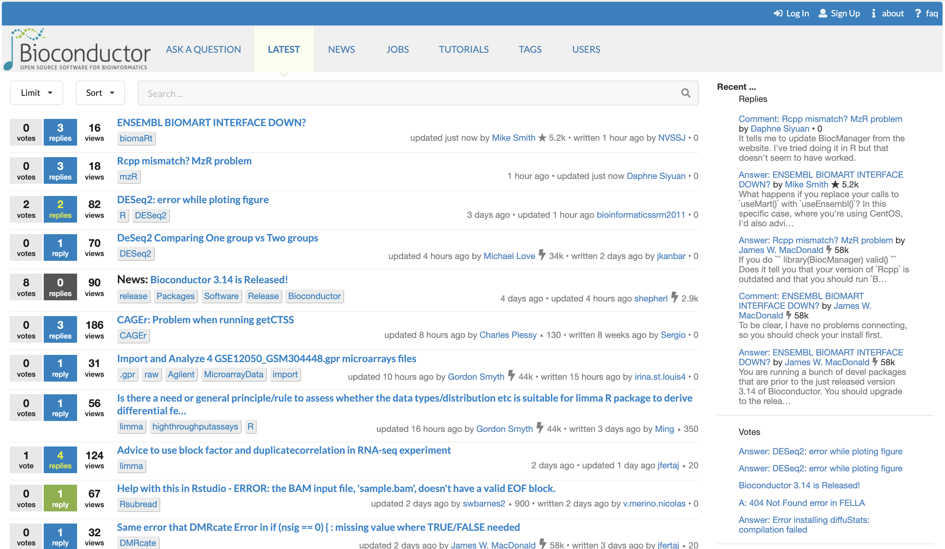
The Bioconductor support site. The Bioconductor support site tracks questions and answers posted by registered users. The platform can be freely browsed and searched by non-registered users.
Workflow packages
Bioconductor workflow packages are special in the way that they are only expected to contain vignettes, without any additional code or functionality of their own. Instead, the vignettes of workflow packages exclusively import functionality from other packages, and demonstrate how to combine functions from those packages into an integrated workflow that users are likely to face in their day-to-day work.
Like regular vignettes, data is typically fetched from publicly available sources, including Bioconductor ExperimentData packages or the Bioconductor ExperimentHub. Those freely available standard data sets allow users to interactively reproduce outputs while they read and follow along the vignette.
Workflow packages can be browsed in a dedicated section of the biocViews page.
Slack workspace
The Bioconductor Slack workspace was created in 2016.
The workspace can be freely joined using this Heroku app to generate invitations for individual email addresses.
The Bioconductor Slack workspace is a lively online platform for official announcements by the Bioconductor Core Team (e.g., Bioconductor release, conferences & events), as well as informal discussions between groups of users subscribed to thematic channels, and direct messages between community members.
The workspace features a large number of channels dedicated to particular topics and areas of interest in the community. Those channels range from active fields of research (e.g., single-cell genomics), to time-limited events (e.g., conferences), but also community outreach (e.g., diversity and representation).
Private channels also exist for governance (e.g., event organisation, advisory boards).
Note
The Slack workspace allows for rapid day-to-day communication and discussion with fellow community members through channels and direct messages.
However, popular channels can reach up to hundreds of users in many different time zones and should be used with parsimony and mindfulness. Conversely, direct messages and private channels are limited to the users invited in the discussion, and any outcome relevant to the community then needs to be re-posted in a public channel.
As a consequence, the Bioconductor support site remains the preferred way to publicly ask questions of interest to the community, in a way that both the question, discussion, and answers are easily searchable and indexed by major search engines.
How to efficiently ask for help
Most community members provide help voluntarily, on their own spare time and without any form of compensation. As such, it is important to ask questions as clearly as possible, providing relevant information, to help those volunteers identify the source of the issue as rapidly as possible, thus saving time for both the helper and the original poster.
Depending on the question, some key information includes:
- Operating system
- Version of R
- Version of Bioconductor
- Version of individual packages installed in the R library
- Version of individual packages attached to the current session
- Third-party software, libraries, and compilers installed on the user’s system
- Source of packages installed in the R library (e.g., Bioconductor, CRAN, GitHub)
- Code executed in the R session leading up to the issue
- Global options active in the session (accessible using
options())
When the issue relates to code being run and producing unexpected outputs, it is paramount to include sufficient information for others to reproduce the issue on their own computer. Indeed, many issues require a live R session to properly investigate the source of the issue, test fixes, or provide workaround and advice.
Crucially, when providing code as part of your post, it is important
that this code be executable by readers, including data that are
processed by the code. Often, the code itself may look correct, while
the issue relates to the interaction between the code and a particular
data set. If sharing sensitive data is not an option, then the issue
should be reformulated and presented using a data set publicly available
on the internet, or including code to generate simulated data randomly
generated in a reproducible way (e.g., set.seed()).
One option is to use the package reprex to collate the code and outputs that describe the issue into formatted text that is easy to post of many online forums, including the Bioconductor support site.
Finally, the Bioconductor support site is the preferred platform to post questions related to Bioconductor packages. This is because questions are visible to the entire community, including many experienced Bioconductor users who regularly answer those questions, and other users who can find answers to questions that were already posted and resolved by the time they run into the issue themselves.
- The
browseVignettes()function is recommended to access the vignette(s) installed with each package. - Vignettes can also be accessed on the Bioconductor website, but beware of differences between package versions!
- The Bioconductor main website contains general information, package documentation, and course materials.
- The Bioconductor support site is the recommended place to contact developers and ask questions.
Content from S4 classes in Bioconductor
Last updated on 2025-10-07 | Edit this page
Overview
Questions
- What is the S4 class system?
- How does Bioconductor use S4 classes?
- How is the Bioconductor
DataFramedifferent from the basedata.frame?
Objectives
- Explain what S4 classes, generics, and methods are.
- Identify S4 classes at the core of the Bioconductor package infrastructure.
- Create various S4 objects and apply relevant S4 methods.
Install packages
Before we can proceed into the following sections, we install some
Bioconductor packages that we will need. First, we check that the BiocManager
package is installed before trying to use it; otherwise we install it.
Then we use the BiocManager::install() function to install
the necessary packages.
R
if (!requireNamespace("BiocManager", quietly = TRUE))
    install.packages("BiocManager")

BiocManager::install("S4Vectors")
For Instructors
The first part of this episode may look somewhat heavy on the theory.
Do not be tempted to go into excessive details about the inner workings
of the S4 class system (e.g., no need to mention the function
new(), or to demonstrate a concrete example of code
creating a class). Instead, the caption of the first figure demonstrates
how to progressively talk through the figure, introducing technical
terms in simple sentences, building up to the method dispatch concept
that is core to the S4 class system, and the source of much confusion in
novice users.
S4 classes and methods
The methods package
The S4 class system is implemented in the base package methods. As such, the concept is not specific to the Bioconductor project and can be found in various independent packages as well. The subject is thoroughly documented in the online book Advanced R, by Hadley Wickham. Most Bioconductor users will never need to get overly familiar with the intricacies of the S4 class system. Rather, the key to an efficient use of packages in the Bioconductor project relies on a sufficient understanding of key motivations for using the S4 class system, as well as best practices for user-facing functionality, including classes, generics, and methods. In the following sections of this episode, we focus on the essential functionality and user experience of S4 classes and methods in the context of the Bioconductor project.
On one side, S4 classes provide data structures capable of storing arbitrarily complex information in computational objects that can be assigned to variable names in an R session. On the other side, S4 generics and methods define functions that may be applied to process those objects.
Over the years, the Bioconductor project has used the S4 class system to develop a number of classes and methods capable of storing and processing data for most biological assays, including raw and processed assay data, experimental metadata for individual features and samples, as well as other assay-specific information as relevant. Gaining familiarity with the standard S4 classes commonly used throughout Bioconductor packages is a key step in building up confidence in users wishing to follow best practices while developing analytical workflows.

S4 classes, generics, and methods. On the left, two
example classes named S4Class1 and S4Class2
demonstrate the concept of inheritance. The class S4Class1
contains two slots named SlotName1 and
SlotName2 for storing data. Those two slots are restricted
to store objects of type SlotType1 and
SlotType2, respectively. The class also defines validity
rules that check the integrity of data each time an object is updated.
The class S4Class2 inherits all the slots and validity
rules from the class S4Class1, in addition to defining a
new slot named SlotName3 and new validity rules. Example
code illustrates how objects of each class are typically created using
constructor functions named identically to the corresponding class. On
the right, one generic function and two methods demonstrate the concept
of polymorphism and the process of S4 method dispatch. The generic
function S4Generic1() defines the name of the function, as
well as its arguments. However, it does not provide any implementation
of that function. Instead, two methods are defined, each providing a
distinct implementation of the generic function for a particular class
of input. Namely, the first method defines an implementation of
S4Generic1() if an object of class S4Class1 is
given as argument x, while the second method method
provides a different implementation of S4Generic1() if an
object of class S4Class2 is given as argument
x. When the generic function S4Generic1() is
called, a process called method dispatch takes
place, whereby the appropriate implementation of the
S4Generic1() method is called according to the class of the
object passed to the argument x.
Slots and validity
In contrast to the S3 class system available directly in base R (not
described in this lesson), the S4 class system provides a much stricter
definition of classes and methods for object-oriented programming (OOP)
in R. Like many programming languages that implement the OOP model, S4
classes are used to represent real-world entities as computational
objects that store information inside one or more internal components
called slots. The class definition declares the type of data
that may be stored in each slot; an error will be thrown if one would
attempt to store unsuitable data. Moreover, the class definition can
also include code that checks the validity of data stored in an object,
beyond their type. For instance, while a slot of type
numeric could be used to store a person’s age, but a
validity method could check that the value stored is, in fact,
positive.
Inheritance
One of the core pillars of the OOP model is the possibility to develop new classes that inherit and extend the functionality of existing classes. The S4 class system implements this paradigm.
The definition of a new S4 classes can declare the name of other classes to inherit from. The new classes will contain all the slots of the parent class, in addition to any new slot added in the definition of the new class itself.
The new class definition can also define new validity checks, which are added to any validity check implement in each of the parent classes.
Generics and methods
While classes define the data structures that store information, generics and methods define the functions that can be applied to objects instantiated from those classes.
S4 generic functions are used to declare the name of functions that are expected to behave differently depending on the class of objects that are given as some of their essential arguments. Instead, S4 methods are used define the distinct implementations of a generic function for each particular combination of inputs.
When a generic function is called and given an S4 object, a process called method dispatch takes place, whereby the class of the object is used to determine the appropriate method to execute.
The S4Vectors package
The S4Vectors
package defines the Vector and List virtual
classes and a set of generic functions that extend the semantic of
ordinary vectors and lists in R. Using the S4 class system, package
developers can easily implement vector-like or list-like objects as
concrete subclasses of Vector or List.
Virtual classes – such as Vector and List –
cannot be instantiated into objects themselves. Instead, those virtual
classes provide core functionality inherited by all the concrete classes
that are derived from them.
Instead, a few low-level concrete subclasses of general interest
(e.g. DataFrame, Rle, and Hits)
are implemented in the S4Vectors
package itself, and many more are implemented in other packages
throughout the Bioconductor project (e.g., IRanges).
Attach the package to the current R session as follows.
R
library(S4Vectors)
Note
The package startup messages printed in the console are worth noting that the S4Vectors package masks a number of functions from the base package when the package is attached to the session. This means that the S4Vectors package includes an implementation of those functions, and that – being the latest package attached to the R session – its own implementation of those functions will be found first on the R search path and used instead of their original implementation in the base package.
In many cases, masked functions can be used as before without any
issue. Occasionally, it may be necessary to disambiguate calls to masked
function using the package name as well as the function name,
e.g. base::anyDuplicated().
The DataFrame class
An extension to the concept of rectangular data
The DataFrame class implemented in the S4Vectors
package extends the concept of rectangular data familiar to users of the
data.frame class in base R, or tibble in the
tidyverse. Specifically, the DataFrame supports the storage
of any type of object (with length and [
methods) as columns.
On the whole, the DataFrame class provides a formal
definition of an S4 class that behaves very similarly to
data.frame, in terms of construction, subsetting,
splitting, combining, etc.
The DataFrame() constructor function should be used to
create new objects, comparably to the data.frame()
equivalent in base R. The help page for the function, accessible as
?DataFrame, can be consulted for more information.
R
DF1 <- DataFrame(
    Integers = c(1L, 2L, 3L),
    Letters = c("A", "B", "C"),
    Floats = c(1.2, 2.3, 3.4)
)
DF1
OUTPUT
DataFrame with 3 rows and 3 columns
   Integers     Letters    Floats
  <integer> <character> <numeric>
1         1           A       1.2
2         2           B       2.3
3         3           C       3.4
In fact, DataFrame objects can be easily converted to
equivalent data.frame objects.
R
df1 <- as.data.frame(DF1)
df1
OUTPUT
  Integers Letters Floats
1        1       A    1.2
2        2       B    2.3
3        3       C    3.4
Vice versa, we can also convert data.frame objects to
DataFrame using the as() function.
R
as(df1, "DataFrame")
OUTPUT
DataFrame with 3 rows and 3 columns
   Integers     Letters    Floats
  <integer> <character> <numeric>
1         1           A       1.2
2         2           B       2.3
3         3           C       3.4
Differences with the base data.frame
The most notable exceptions have to do with handling of row names.
First, row names are optional. This means calling
rownames(x) will return NULL if there are no
row names.
R
rownames(DF1)
OUTPUT
NULLThis is different from data.frame, where
rownames(x) returns the equivalent of
as.character(seq_len(nrow(x))).
R
rownames(df1)
OUTPUT
[1] "1" "2" "3"However, returning NULL informs, for example,
combination functions that no row names are desired (they are often a
luxury when dealing with large data).
Furthermore, row names of DataFrame objects are not
required to be unique, in contrast to the data.frame in
base R. Row names are a frequent source of controversy in R, as they can
be used to uniquely identify and index observations in rectangular
format, without storing that information explicitly in a dedicated
column. When set, row names can be used to subset rectangular data using
the [ operator. Meanwhile, non-unique row names defeat that
purpose and can lead to unexpected results, as only the first occurrence
of each selected row name is extracted. Instead, the tidyverse
tibble removed the ability to set row names altogether,
forcing users to store every bit of information explicitly in dedicated
columns, while providing functions to dedicated to efficiently filtering
rows in rectangular data, without the need for the [
operator.
R
DF2 <- DataFrame(
    Integers = c(1L, 2L, 3L),
    Letters = c("A", "B", "C"),
    Floats = c(1.2, 2.3, 3.4),
    row.names = c("name1", "name1", "name2")
)
DF2
OUTPUT
DataFrame with 3 rows and 3 columns
       Integers     Letters    Floats
      <integer> <character> <numeric>
name1         1           A       1.2
name1         2           B       2.3
name2         3           C       3.4
Challenge
Using the example above, what does DF2["name1", ]
return? Why?
> DF2["name1", ]
DataFrame with 1 row and 3 columns
       Integers     Letters    Floats
      <integer> <character> <numeric>
name1         1           A       1.2
Only the first occurrence of a row matching the row name
name1 is returned.
In this case, row names do not have a particular meaning, making it
difficult to justify the need for them. Instead, users could extract all
the rows that matching the row name name1 more explicitly
as follows: DF2[rownames(DF2) == "name1", ].
Users should be mindful of the motivation for using row names in any given situation; what they represent, and how they should be used during the analysis.
Finally, row names in DataFrame do not support partial
matching during subsetting, in contrast to data.frame. The
stricter behaviour of DataFrame prevents often unexpected
results faced by unsuspecting users.
R
DF3 <- DataFrame(
    Integers = c(1L, 2L, 3L),
    Letters = c("A", "B", "C"),
    Floats = c(1.2, 2.3, 3.4),
    row.names = c("alpha", "beta", "gamma")
)
df3 <- as.data.frame(DF3)
Challenge
Using the examples above, what are the outputs of
DF3["a", ] and df3["a", ]? Why are they
different?
> DF3["a", ]
DataFrame with 1 row and 3 columns
      Integers     Letters    Floats
     <integer> <character> <numeric>
<NA>        NA          NA        NA
> df3["a", ]
      Integers Letters Floats
alpha        1       A    1.2
The DataFrame object did not perform partial row name
matching, and thus did not match any row and return a
DataFrame full of NA values. Instead, the
data.frame object performed partial row name matching,
matched the requested "a" to the "alpha" row
name, and returned the corresponding row as a new
data.frame object.
Indexing
Just like a regular data.frame, columns can be accessed
using $, [, and [[. Each operator
has a different purpose, and the most appropriate one will often depend
on what you are trying to achieve.
For example, the dollar operator $ can be used to
extract a single column by name. That will often be a vector, but it may
depend on the nature of the data in that column. This operator can be
quite convenient in an interactive R session, as it will offer
autocompletion among available column names.
R
DF3$Integers
OUTPUT
[1] 1 2 3Similarly, the double bracket operator [[ can also be
used to extract a single column. It is more flexible than $
as it can handle both character names and integer indices.
R
DF3[["Letters"]]
OUTPUT
[1] "A" "B" "C"R
DF3[[2]]
OUTPUT
[1] "A" "B" "C"The operator [ is most convenient when it comes to
selecting simultaneously on rows and columns, or controlling whether a
single-column selection should be returned as a DataFrame
or a vector.
R
DF3[2:3, "Letters", drop=FALSE]
OUTPUT
DataFrame with 2 rows and 1 column
          Letters
      <character>
beta            B
gamma           C
Metadata columns
One of most notable novel functionality in DataFrame
relative to the base data.frame is the capacity to hold
metadata on the columns in another DataFrame.

Metadata columns. Metadata columns are illustrated
in the context of a DataFrame object. On the left, a
DataFrame object called DF is created with
columns named A and B. On the right, the
metadata columns for DF are accessed using
mcols(DF). In this example, two metadata columns are
created with names meta1 and meta2. Metadata
columns are stored as a DataFrame that contains one row for
each column in the parent DataFrame.
The metadata columns are accessed using the function
mcols(), If no metadata column is defined,
mcols() simply returns NULL.
R
DF4 <- DataFrame(
    Integers = c(1L, 2L, 3L),
    Letters = c("A", "B", "C"),
    Floats = c(1.2, 2.3, 3.4),
    row.names = c("alpha", "beta", "gamma")
)
mcols(DF4)
OUTPUT
NULLThe function mcols() can also be used to add, edit, or
remove metadata columns. For instance, we can initialise metadata
columns as a DataFrame of two columns:
- one column indicating the type of value stored in the corresponding column
- one column indicating the number of distinct values observed in the corresponding column
R
mcols(DF4) <- DataFrame(
    Type = sapply(DF4, typeof),
    Distinct = sapply(DF4, function(x) { length(unique(x)) } )
)
mcols(DF4)
OUTPUT
DataFrame with 3 rows and 2 columns
                Type  Distinct
         <character> <integer>
Integers     integer         3
Letters    character         3
Floats double 3Note
The row names of the metadata columns are automatically set to match
the column names of the parent DataFrame, clearly
indicating the pairing between columns and metadata.
Run-length encoding (RLE)
An extension to the concept of vector
Similarly to the DataFrame class implemented in the
S4Vectors,
the Rle class provides an S4 extension to the
rle() function from the base package. Specifically, the
Rle class supports the storage of atomic vectors in a
run-length encoding format.

Run-length encoding. The concept of run-length encoding is demonstrated here using the example of a sequence of nucleic acids. Before encoding, each nucleotide at each position in the sequence is explicitly stored in memory. During the encoding, consecutive runs of identical nucleotides are collapsed into two bits of information: the identity of the nucleotide and the length of the run.
Run-length encoding can dramatically reduce the memory footprint of
vectors that contain frequent runs of identical information. For
instance, a compelling application of run-length encoding is the
representation of genomic coverage in sequencing experiments, where
large genomic regions devoid of any mapped reads result in long runs of
0 values. Storing each individual value would be highly
inefficient from the standpoint of memory usage. Instead, the run-length
encoding process collapses such runs of redundant information from
arbitrarily long runs of identical information to two values: the
repeated value itself, and the number of times that it is repeated.
R
v1 <- c(0, 0, 0, 0, 0, 0, 0, 1, 2, 3, 2, 1, 0, 0, 0, 0, 0)
rle1 <- Rle(v1)
rle1
OUTPUT
numeric-Rle of length 17 with 7 runs
  Lengths: 7 1 1 1 1 1 5
  Values : 0 1 2 3 2 1 0
Indexing
Just like a regular vector, Rle objects can
be indexed using [.
R
rle1[2:4]
OUTPUT
numeric-Rle of length 3 with 1 run
  Lengths: 3
  Values : 0
Usage
As vector-like objects, Rle objects can also be stored
as columns of DataFrame objects, alongside other
vector-like objects.
R
v2 <- c(rep(1, 5), rep(2, 5))
rle2 <- Rle(v2)
DF5 <- DataFrame(
    vector = v2,
    rle = rle2,
    equal = v2 == rle2
)
DF5
OUTPUT
DataFrame with 10 rows and 3 columns
      vector   rle equal
   <numeric> <Rle> <Rle>
1          1     1  TRUE
2          1     1  TRUE
3          1     1  TRUE
4          1     1  TRUE
5          1     1  TRUE
6          2     2  TRUE
7          2     2  TRUE
8          2     2  TRUE
9          2     2  TRUE
10 2 2 TRUEGoing further
A number of standard operations with Rle objects are
documented in the help page of the Rle class, accessible as
?Rle, and in the vignettes of the S4Vectors
package, accessible using browseVignettes("S4Vectors").
- S4 classes store information in slots, and check the validity of the information every an object is updated.
- To ensure the continued integrity of S4 objects, users should not access slots directly, but using dedicated functions.
- S4 generics invoke different implementations of the method depending on the class of the object that they are given.
- The S4 class
DataFrameextends the functionality of basedata.frame, for instance with the capacity to hold information about each column in metadata columns. - The S4 class
Rleextends the functionality of the basevector, for instance with the capacity to encode repetitive vectors in a memory-efficient format.
Content from Working with biological sequences
Last updated on 2025-10-07 | Edit this page
Overview
Questions
- What is the recommended way to represent biological sequences in Bioconductor?
- What Bioconductor packages provides methods to efficiently process biological sequences?
Objectives
- Explain how biological sequences are represented in the Bioconductor project.
- Identify Bioconductor packages and methods available to process biological sequences.
Install packages
Before we can proceed into the following sections, we install some
Bioconductor packages that we will need. First, we check that the BiocManager
package is installed before trying to use it; otherwise we install it.
Then we use the BiocManager::install() function to install
the necessary packages.
R
if (!requireNamespace("BiocManager", quietly = TRUE))
    install.packages("BiocManager")

BiocManager::install("Biostrings")
The Biostrings package and classes
Why do we need classes for biological sequences?
Biological sequences are arguably some of the simplest biological entities to represent computationally. Examples include nucleic acid sequences (e.g., DNA, RNA) and protein sequences composed of amino acids.
That is because alphabets have been designed and agreed upon to represent individual monomers using character symbols.
For instance, using the alphabet for amino acids, the reference protein sequence for the Actin, alpha skeletal muscle protein sequence is represented as follows.
OUTPUT
[1] "MCDEDETTALVCDNGSGLVKAGFAGDDAPRAVFPSIVGRPRHQGVMVGMGQKDSYVGDEAQSKRGILTLKYPIEHGIITNWDDMEKIWHHTFYNELRVAPEEHPTLLTEAPLNPKANREKMTQIMFETFNVPAMYVAIQAVLSLYASGRTTGIVLDSGDGVTHNVPIYEGYALPHAIMRLDLAGRDLTDYLMKILTERGYSFVTTAEREIVRDIKEKLCYVALDFENEMATAASSSSLEKSYELPDGQVITIGNERFRCPETLFQPSFIGMESAGIHETTYNSIMKCDIDIRKDLYANNVMSGGTTMYPGIADRMQKEITALAPSTMKIKIIAPPERKYSVWIGGSILASLSTFQQMWITKQEYDEAGPSIVHRKCF"However, a major limitation of regular character vectors is that they do not check the validity of the sequences that they contain. Practically, it is possible to store meaningless sequences of symbols in character strings, including symbols that are not part of the official alphabet for the relevant type of polymer. In those cases, the burden of checking the validity of sequences falls on the programs that process them, or causing those programs to run into errors when they unexpectedly encounter invalid symbols in a sequence.
Instead, S4 classes – demonstrated in the earlier episode The S4 class system – provide a way to label objects as distinct “DNA”, “RNA”, or “protein” varieties of biological sequences. This label is an extremely powerful way to inform programs on the set of character symbols they can expect in the sequence, but also the range of computational operations that can be applied to those sequences. For instance, a function designed to translate nucleic acid sequences into the corresponding amino acid sequence should only be allowed to run on sequences that represent nucleic acids.
Challenge
Can you tell whether this character string is a valid DNA sequence?
AATTGGCCRGGCCAATTYes, this is a valid DNA sequence using ambiguity codes defined in
the IUPAC
notation. In this case, A, T, C,
and G represents the four standard types of nucleotides,
while the R symbol acts as a regular expression
representing either of the two purine nucleotide bases, A
and G.
The Biostrings package
Overview
In the Bioconductor project, the Biostrings
package implements S4 classes to represent biological sequences as S4
objects, e.g. DNAString for sequences of nucleotides in
deoxyribonucleic acid polymers, and AAString for sequences
of amino acids in protein polymers. Those S4 classes provide
memory-efficient containers for character strings, automatic
validity-checking functionality for each class of biological molecules,
and methods implementing various string matching algorithms and other
utilities for fast manipulation and processing of large biological
sequences or sets of sequences.
A short presentation of the basic classes defined in the Biostrings
package is available in one of the package vignettes, accessible as
vignette("Biostrings2Classes"), while more detailed
information is provided in the other package vignettes, accessible as
browseVignettes("Biostrings").
First steps
To get started, we load the package.
R
library(Biostrings)
With the package loaded and attached to the session, we have access
to the package functions. Those include functions that let us create new
objects of the classes defined in the package. For instance, we can
create an object that represents a DNA sequence, using the
DNAString() constructor function. Without assigning the
output to an object, we let the resulting object be printed in the
console.
R
DNAString("ATCG")
OUTPUT
4-letter DNAString object
seq: ATCG
Notably, DNA sequences may only contain the symbols A,
T, C, and G, to represent the
four DNA nucleotide bases, the symbol N as a placeholder
for an unknown or unspecified base, and a restricted set of additional
symbols with special meaning defined in the IUPAC Extended
Genetic Alphabet. Notice that the constructor function does not let
us create objects that contain invalid characters,
e.g. Z.
R
DNAString("ATCGZ")
ERROR
Error in .Call2("new_XString_from_CHARACTER", class(x0), string, start, : key 90 (char 'Z') not in lookup tableSpecifically, the IUPAC Extended
Genetic Alphabet defines ambiguity codes that represent sets of
nucleotides, in a way similar to regular expressions. The
IUPAC_CODE_MAP named character vector contains the mapping
from the IUPAC nucleotide ambiguity codes to their meaning.
R
IUPAC_CODE_MAP
OUTPUT
     A      C      G      T      M      R      W      S      Y      K      V
   "A"    "C"    "G"    "T"   "AC"   "AG"   "AT"   "CG"   "CT"   "GT"  "ACG"
     H      D      B      N
 "ACT"  "AGT"  "CGT" "ACGT"
Any of those nucleotide codes are allowed in the sequence of a
DNAString object. For instance, the symbol M
represents either of the two nucleotides A or
C at a given position in a nucleic acid sequence.
R
DNAString("ATCGM")
OUTPUT
5-letter DNAString object
seq: ATCGM
In particular, pattern matching methods implemented in the Biostrings
package recognize the meaning of ambiguity codes for each class of
biological sequence, allowing them to efficiently match motifs queried
by users without the need to design elaborate regular expressions. For
instance, the method matchPattern() takes a
pattern= and a subject= argument, and returns
a Views object that reports and displays any match of the
pattern expression at any position in the
subject sequence.
Note that the default option fixed = TRUE instructs the
method to match the query exactly – i.e., ignore ambiguity codes – which
in this case does not report any exact match.
R
dna1 <- DNAString("ATCGCTTTGA")
matchPattern("GM", dna1, fixed = TRUE)
OUTPUT
Views on a 10-letter DNAString subject
subject: ATCGCTTTGA
views: NONE
Instead, to indicate that the pattern includes some ambiguity code,
the argument fixed must be set to FALSE.
R
matchPattern("GM", dna1, fixed = FALSE)
OUTPUT
Views on a 10-letter DNAString subject
subject: ATCGCTTTGA
views:
      start end width
  [1]     4   5     2 [GC]
  [2]     9  10     2 [GA]
In this particular example, two views describe matches of the pattern
in the subject sequence. Specifically, the pattern GM first
matched the sequence GC spanning positions 4 to 5 in the
subject sequence, and then also matched the sequence GA
from positions 9 to 10.
Similarly to the method matchPattern(), the method
countPattern() can be applied to simply count the number of
matches of the pattern in the subject
sequence. And again, the option fixed controls whether to
respect ambiguity codes, or match them exactly.
Challenge
How many hits does the following code return? Why?
dna2 <- DNAString("TGATTGCTTGGTTGMTT")
countPattern("GM", dna2, fixed = FALSE)The method countPattern() reports 3 hits, because the
option fixed = FALSE allows the pattern GM to
match GA, GC, and GM sequences,
due to the use of the ambiguity code M in the
pattern.
Importing biological strings from files
In practice, users rarely type the strings representing biological sequences themselves. Most of the time, biological strings are imported from files, either downloaded from public repositories or generated locally using bioinformatics programs.
For instance, we can load the set of adapter sequences for the TruSeq™
DNA PCR-Free whole-genome sequencing library preparation kit from a
file that we downloaded during the lesson setup. Since adapter sequences
are nucleic acid sequences, we must use the function
readDNAStringSet().
R
truseq_adapters <- readDNAStringSet(filepath = "data/TruSeq3-PE-2.fa")
truseq_adapters
OUTPUT
DNAStringSet object of length 6:
    width seq                                               names
[1]    34 TACACTCTTTCCCTACACGACGCTCTTCCGATCT                PrefixPE/1
[2]    34 GTGACTGGAGTTCAGACGTGTGCTCTTCCGATCT                PrefixPE/2
[3]    34 TACACTCTTTCCCTACACGACGCTCTTCCGATCT                PE1
[4]    34 AGATCGGAAGAGCGTCGTGTAGGGAAAGAGTGTA                PE1_rc
[5]    34 GTGACTGGAGTTCAGACGTGTGCTCTTCCGATCT                PE2
[6] 34 AGATCGGAAGAGCACACGTCTGAACTCCAGTCAC PE2_rcGoing further
The help page of the function readDNAStringSet() –
accessible using help(readDNAStringSet) – documents related
functions designed to import other types of biological sequences, e.g
readRNAStringSet(), readAAStringSet().
Operations on biological strings
Computing the frequency of symbols
The Biostrings
package provides several functions to process and manipulate classes of
biological strings. For example, we have come across
matchPattern() and countPattern() earlier in
this episode.
Another example of a method that can be applied to biological strings
is letterFrequency(), to compute the frequency of letters
in a biological sequence.
R
letterFrequency(truseq_adapters, letters = DNA_ALPHABET)
OUTPUT
      A  C  G  T M R W S Y K V H D B N - + .
[1,]  6 14  3 11 0 0 0 0 0 0 0 0 0 0 0 0 0 0
[2,]  5  8 10 11 0 0 0 0 0 0 0 0 0 0 0 0 0 0
[3,]  6 14  3 11 0 0 0 0 0 0 0 0 0 0 0 0 0 0
[4,] 11  3 14  6 0 0 0 0 0 0 0 0 0 0 0 0 0 0
[5,]  5  8 10 11 0 0 0 0 0 0 0 0 0 0 0 0 0 0
[6,] 11 10  8  5 0 0 0 0 0 0 0 0 0 0 0 0 0 0
The output is a matrix with one row for each sequence in the
DNAStringSet object, and one column for each symbol in the
alphabet of deoxyribonucleic acids, provided by the Biostrings
package in a built-in object called DNA_ALPHABET.
Amino acid sequences
Similarly to the DNAString and DNAStringSet
classes, the classes AAString and AAStringSet
allow efficient storage and manipulation of a long amino acid sequence,
or a set thereof.
Similarly to built-in objects for the DNA alphabet, the built-in
objects AA_ALPHABET, AA_STANDARD and
AA_PROTEINOGENIC describe different subsets of the alphabet
of valid symbols for amino acid sequences.
For instance, the AA_ALPHABET object describes the set
of symbols in the full amino acid alphabet.
R
AA_ALPHABET
OUTPUT
 [1] "A" "R" "N" "D" "C" "Q" "E" "G" "H" "I" "L" "K" "M" "F" "P" "S" "T" "W" "Y"
[20] "V" "U" "O" "B" "J" "Z" "X" "*" "-" "+" "."
Challenge
Use base R code to identify the two symbols present in the
AA_PROTEINOGENIC alphabet object that are absent from the
AA_STANDARD alphabet object. What do those two symbols
represent?
> setdiff(AA_PROTEINOGENIC, AA_STANDARD)
[1] "U" "O"
The symbols U and O represent
selenocysteine and pyrrolysine, respectively. Those two amino acids are
in some species coded for by codons that are usually interpreted as stop
codons. As such, they are not included in the alphabet of “standard”
amino acids, and an alphabet of “proteinogenic” amino acids was defined
to acknowledge the special biology of those amino acids. Either of those
alphabets may be used to determine the validity of an amino acid
sequence, depending on its biological nature.
Translating nucleotide sequences
One of the key motivations for the use of S4 classes and the object-oriented programming (OOP) model relies on the infrastructure of S4 generics and methods. As described in the earlier episode The S4 class system, generics provide a mechanism for defining and applying distinct implementations of the same generic function name, according to the nature of the input object(s) provided to the function call.
For instance, the Biostrings
package provides multiple implementations of a generic called
translate(), for translating DNA or RNA sequences into
amino acid sequences. The set of input objects supported by the generic
translate() can be listed using the function
showMethods(), from the CRAN package methods.
R
showMethods("translate")
OUTPUT
Function: translate (package Biostrings)
x="DNAString"
x="DNAStringSet"
x="MaskedDNAString"
x="MaskedRNAString"
x="RNAString"
x="RNAStringSet"
In the output above, we see that that the generic function
translate() includes methods capable of handling objects
representing DNA and RNA sequences in the DNAString and
RNAString classes, respectively; but also lists of DNA and
RNA sequences in objects of class DNAStringSet and
RNAStringSet, as well as other classes capable of storing
DNA and RNA sequences.
To demonstrate the use of the translate() method, we
first load a set of open reading frames (ORFs) identified by the NIH Open Reading Frame
Finder for the Homo sapiens actin beta (ACTB) mRNA (RefSeq:
NM_001101), using the standard genetic code, a minimal ORF length of 75
nucleotides, and starting with the “ATG” start codon only.
R
actb_orf_nih <- readDNAStringSet("data/actb_orfs.fasta")
actb_orf_nih
OUTPUT
DNAStringSet object of length 13:
     width seq                                              names
 [1]   222 ATGCCCACCATCACGCCCTGGTG...CGGGGCGGACGCGGTCTCGGCG gi|1519311456|ref...
 [2]  1128 ATGGATGATGATATCGCCGCGCT...CGTCCACCGCAAATGCTTCTAG gi|1519311456|ref...
 [3]   126 ATGATGATATCGCCGCGCTCGTC...CGCCCCAGGCACCAGGGCGTGA gi|1519311456|ref...
 [4]    90 ATGTCGTCCCAGTTGGTGACGAT...CTGGGCCTCGTCGCCCACATAG gi|1519311456|ref...
 [5]   225 ATGGGCACAGTGTGGGTGACCCC...AGCCACACGCAGCTCATTGTAG gi|1519311456|ref...
 ...   ... ...
 [9]   342 ATGAGATTGGCATGGCTTTATTT...ATGTAATGCAAAATTTTTTTAA gi|1519311456|ref...
[10]   168 ATGGCTTTATTTGTTTTTTTTGT...TTGCACATTGTTGTTTTTTTAA gi|1519311456|ref...
[11]   111 ATGACTATTAAAAAAACAACAAT...CCTTCACCGTTCCAGTTTTTAA gi|1519311456|ref...
[12]   105 ATGCAAAATTTTTTTAATCTTCG...CCTTTTTTGTCCCCCAACTTGA gi|1519311456|ref...
[13]   135 ATGATGAGCCTTCGTGCCCCCCC...TGACTTGAGACCAGTTGAATAA gi|1519311456|ref...
Having imported the nucleotide sequences as a
DNAStringSet object, we can apply the
translate() method to that object to produce the amino acid
sequence that results from the translation process for each nucleotide
sequence.
R
actb_aa <- translate(actb_orf_nih)
actb_aa
OUTPUT
AAStringSet object of length 13:
     width seq                                              names
 [1]    74 MPTITPWCLGRPTMEGKTARGAS...VWTGGGSAKARLCARGADAVSA gi|1519311456|ref...
 [2]   376 MDDDIAALVVDNGSGMCKAGFAG...MWISKQEYDESGPSIVHRKCF* gi|1519311456|ref...
 [3]    42 MMISPRSSSTTAPACARPASRATMPPGPSSPPSWGAPGTRA*       gi|1519311456|ref...
 [4]    30 MSSQLVTMPCSMGYFRVRMPLLLWASSPT*                   gi|1519311456|ref...
 [5]    75 MGTVWVTPSPESITMPVVRPEAY...GFRGASVSSTGCSSGATRSSL* gi|1519311456|ref...
 ...   ... ...
 [9]   114 MRLAWLYLFFLFCFGFFFFFGLT...QVHTGEVIALLSCKLCNAKFF* gi|1519311456|ref...
[10]    56 MALFVFFVLFWFFFFFWLDSGFK...ERASPKVHNVAEDFDCTLLFF* gi|1519311456|ref...
[11]    37 MTIKKTTMCNQSPRPHCELWGMLAPTDCCHLHRSSF*            gi|1519311456|ref...
[12]    35 MQNFFNLRLNTFLFCFILNDEPSCPPFPLFCPPT*              gi|1519311456|ref...
[13]    45 MMSLRAPPSPFFVPQLEMYEGFWSPWEWVEAARAYLYTDLRPVE*    gi|1519311456|ref...
In the example above, all amino acid sequences visible start with the
typical methionin amino acid encoded by the “ATG” start codon. We also
see that all but one of the amino acid sequences visible end with the
* symbol, which indicates that the translation process
ended on a stop codon. In contrast, the first open reading frame above
reached the end of the nucleotide sequence without encoutering a stop
codon.
Conveniently, the number of amino acids in each sequence is stated
under the header width.
Challenge
Extract the length of each amino acid sequence above as an integer vector. What is the length of the longest amino acid sequence translated from any of those open reading frames?
Compare your result with the sequence information on the UniPro page for ACTB (https://www.uniprot.org/uniprot/P60709#sequences).
width(actb_aa)
# or
max(width(actb_aa))
The longest translated sequence contains 376 amino acids.
The Uniprot page reports a sequence of 375 amino acids. However, the
UniProt amino acid sequence does not comprise any symbol to represent
the stop codon. That difference aside, the UniPro amino acid sequence is
identical to the sequence that was produced by the
translate() method.
The BSgenome package
Overview
In the Bioconductor project, the BSgenome package provides software infrastructure for efficient representation of full genome and their single-nucleotide polymorphisms.
The BSgenome package itself does not contain any genome sequence itself, but provides functionality to access genome sequences available in other Bioconductor packages, as we demonstrate in the next section.
First steps
To get started, we load the package.
R
library(BSgenome)
With the package loaded and attached to the session, we have access to the package functions.
In particular, the function
BSgenome::available.genomes() can be used to display the
names of Bioconductor packages that contain genome sequences.
R
available.genomes()
OUTPUT
'getOption("repos")' replaces Bioconductor standard repositories, see
'help("repositories", package = "BiocManager")' for details.
Replacement repositories:
    BioCsoft: https://bioconductor.org/packages/3.19/bioc
    BioCann: https://bioconductor.org/packages/3.19/data/annotation
    BioCexp: https://bioconductor.org/packages/3.19/data/experiment
    BioCworkflows: https://bioconductor.org/packages/3.19/workflows
    BioCbooks: https://bioconductor.org/packages/3.19/books
    CRAN: https://cloud.r-project.org
OUTPUT
  [1] "BSgenome.Alyrata.JGI.v1"
  [2] "BSgenome.Amellifera.BeeBase.assembly4"
  [3] "BSgenome.Amellifera.NCBI.AmelHAv3.1"
  [4] "BSgenome.Amellifera.UCSC.apiMel2"
  [5] "BSgenome.Amellifera.UCSC.apiMel2.masked"
  [6] "BSgenome.Aofficinalis.NCBI.V1"
  [7] "BSgenome.Athaliana.TAIR.04232008"
  [8] "BSgenome.Athaliana.TAIR.TAIR9"
  [9] "BSgenome.Btaurus.UCSC.bosTau3"
 [10] "BSgenome.Btaurus.UCSC.bosTau3.masked"
 [11] "BSgenome.Btaurus.UCSC.bosTau4"
 [12] "BSgenome.Btaurus.UCSC.bosTau4.masked"
 [13] "BSgenome.Btaurus.UCSC.bosTau6"
 [14] "BSgenome.Btaurus.UCSC.bosTau6.masked"
 [15] "BSgenome.Btaurus.UCSC.bosTau8"
 [16] "BSgenome.Btaurus.UCSC.bosTau9"
 [17] "BSgenome.Btaurus.UCSC.bosTau9.masked"
 [18] "BSgenome.Carietinum.NCBI.v1"
 [19] "BSgenome.Celegans.UCSC.ce10"
 [20] "BSgenome.Celegans.UCSC.ce11"
 [21] "BSgenome.Celegans.UCSC.ce2"
 [22] "BSgenome.Celegans.UCSC.ce6"
 [23] "BSgenome.Cfamiliaris.UCSC.canFam2"
 [24] "BSgenome.Cfamiliaris.UCSC.canFam2.masked"
 [25] "BSgenome.Cfamiliaris.UCSC.canFam3"
 [26] "BSgenome.Cfamiliaris.UCSC.canFam3.masked"
 [27] "BSgenome.Cjacchus.UCSC.calJac3"
 [28] "BSgenome.Cjacchus.UCSC.calJac4"
 [29] "BSgenome.CneoformansVarGrubiiKN99.NCBI.ASM221672v1"
 [30] "BSgenome.Creinhardtii.JGI.v5.6"
 [31] "BSgenome.Dmelanogaster.UCSC.dm2"
 [32] "BSgenome.Dmelanogaster.UCSC.dm2.masked"
 [33] "BSgenome.Dmelanogaster.UCSC.dm3"
 [34] "BSgenome.Dmelanogaster.UCSC.dm3.masked"
 [35] "BSgenome.Dmelanogaster.UCSC.dm6"
 [36] "BSgenome.Drerio.UCSC.danRer10"
 [37] "BSgenome.Drerio.UCSC.danRer11"
 [38] "BSgenome.Drerio.UCSC.danRer5"
 [39] "BSgenome.Drerio.UCSC.danRer5.masked"
 [40] "BSgenome.Drerio.UCSC.danRer6"
 [41] "BSgenome.Drerio.UCSC.danRer6.masked"
 [42] "BSgenome.Drerio.UCSC.danRer7"
 [43] "BSgenome.Drerio.UCSC.danRer7.masked"
 [44] "BSgenome.Dvirilis.Ensembl.dvircaf1"
 [45] "BSgenome.Ecoli.NCBI.20080805"
 [46] "BSgenome.Gaculeatus.UCSC.gasAcu1"
 [47] "BSgenome.Gaculeatus.UCSC.gasAcu1.masked"
 [48] "BSgenome.Ggallus.UCSC.galGal3"
 [49] "BSgenome.Ggallus.UCSC.galGal3.masked"
 [50] "BSgenome.Ggallus.UCSC.galGal4"
 [51] "BSgenome.Ggallus.UCSC.galGal4.masked"
 [52] "BSgenome.Ggallus.UCSC.galGal5"
 [53] "BSgenome.Ggallus.UCSC.galGal6"
 [54] "BSgenome.Gmax.NCBI.Gmv40"
 [55] "BSgenome.Hsapiens.1000genomes.hs37d5"
 [56] "BSgenome.Hsapiens.NCBI.GRCh38"
 [57] "BSgenome.Hsapiens.NCBI.T2T.CHM13v2.0"
 [58] "BSgenome.Hsapiens.UCSC.hg17"
 [59] "BSgenome.Hsapiens.UCSC.hg17.masked"
 [60] "BSgenome.Hsapiens.UCSC.hg18"
 [61] "BSgenome.Hsapiens.UCSC.hg18.masked"
 [62] "BSgenome.Hsapiens.UCSC.hg19"
 [63] "BSgenome.Hsapiens.UCSC.hg19.masked"
 [64] "BSgenome.Hsapiens.UCSC.hg38"
 [65] "BSgenome.Hsapiens.UCSC.hg38.dbSNP151.major"
 [66] "BSgenome.Hsapiens.UCSC.hg38.dbSNP151.minor"
 [67] "BSgenome.Hsapiens.UCSC.hg38.masked"
 [68] "BSgenome.Hsapiens.UCSC.hs1"
 [69] "BSgenome.Mdomestica.UCSC.monDom5"
 [70] "BSgenome.Mfascicularis.NCBI.5.0"
 [71] "BSgenome.Mfascicularis.NCBI.6.0"
 [72] "BSgenome.Mfuro.UCSC.musFur1"
 [73] "BSgenome.Mmulatta.UCSC.rheMac10"
 [74] "BSgenome.Mmulatta.UCSC.rheMac2"
 [75] "BSgenome.Mmulatta.UCSC.rheMac2.masked"
 [76] "BSgenome.Mmulatta.UCSC.rheMac3"
 [77] "BSgenome.Mmulatta.UCSC.rheMac3.masked"
 [78] "BSgenome.Mmulatta.UCSC.rheMac8"
 [79] "BSgenome.Mmusculus.UCSC.mm10"
 [80] "BSgenome.Mmusculus.UCSC.mm10.masked"
 [81] "BSgenome.Mmusculus.UCSC.mm39"
 [82] "BSgenome.Mmusculus.UCSC.mm8"
 [83] "BSgenome.Mmusculus.UCSC.mm8.masked"
 [84] "BSgenome.Mmusculus.UCSC.mm9"
 [85] "BSgenome.Mmusculus.UCSC.mm9.masked"
 [86] "BSgenome.Osativa.MSU.MSU7"
 [87] "BSgenome.Ppaniscus.UCSC.panPan1"
 [88] "BSgenome.Ppaniscus.UCSC.panPan2"
 [89] "BSgenome.Ptroglodytes.UCSC.panTro2"
 [90] "BSgenome.Ptroglodytes.UCSC.panTro2.masked"
 [91] "BSgenome.Ptroglodytes.UCSC.panTro3"
 [92] "BSgenome.Ptroglodytes.UCSC.panTro3.masked"
 [93] "BSgenome.Ptroglodytes.UCSC.panTro5"
 [94] "BSgenome.Ptroglodytes.UCSC.panTro6"
 [95] "BSgenome.Rnorvegicus.UCSC.rn4"
 [96] "BSgenome.Rnorvegicus.UCSC.rn4.masked"
 [97] "BSgenome.Rnorvegicus.UCSC.rn5"
 [98] "BSgenome.Rnorvegicus.UCSC.rn5.masked"
 [99] "BSgenome.Rnorvegicus.UCSC.rn6"
[100] "BSgenome.Rnorvegicus.UCSC.rn7"
[101] "BSgenome.Scerevisiae.UCSC.sacCer1"
[102] "BSgenome.Scerevisiae.UCSC.sacCer2"
[103] "BSgenome.Scerevisiae.UCSC.sacCer3"
[104] "BSgenome.Sscrofa.UCSC.susScr11"
[105] "BSgenome.Sscrofa.UCSC.susScr3"
[106] "BSgenome.Sscrofa.UCSC.susScr3.masked"
[107] "BSgenome.Tgondii.ToxoDB.7.0"
[108] "BSgenome.Tguttata.UCSC.taeGut1"
[109] "BSgenome.Tguttata.UCSC.taeGut1.masked"
[110] "BSgenome.Tguttata.UCSC.taeGut2"
[111] "BSgenome.Vvinifera.URGI.IGGP12Xv0"
[112] "BSgenome.Vvinifera.URGI.IGGP12Xv2"
[113] "BSgenome.Vvinifera.URGI.IGGP8X"
Installing BSgenome packages
To use one of the available genomes, the corresponding package must
be installed first. For instance, the example below demonstrates how the
data package BSgenome.Hsapiens.UCSC.hg38.masked
can be installed using the function BiocManager::install()
that we have seen before.
R
BiocManager::install("BSgenome.Hsapiens.UCSC.hg38.masked")
Using BSgenome packages
Once installed, BSgenome packages can be loaded like any other R
package, using the library() function.
R
library(BSgenome.Hsapiens.UCSC.hg38.masked)
Each BSgenome package contains an object that is named identically to the package and contains the genome sequence.
Having loaded the package BSgenome.Hsapiens.UCSC.hg38.masked above, we can display the BSgenome object as follows.
R
BSgenome.Hsapiens.UCSC.hg38.masked
OUTPUT
| BSgenome object for Human
| - organism: Homo sapiens
| - provider: UCSC
| - genome: hg38
| - release date: 2023/01/31
| - 711 sequence(s):
|     chr1                    chr2                    chr3
|     chr4                    chr5                    chr6
|     chr7                    chr8                    chr9
|     chr10                   chr11                   chr12
|     chr13                   chr14                   chr15
|     ...                     ...                     ...
|     chr19_KV575256v1_alt    chr19_KV575257v1_alt    chr19_KV575258v1_alt
|     chr19_KV575259v1_alt    chr19_KV575260v1_alt    chr19_MU273387v1_alt
|     chr22_KN196485v1_alt    chr22_KN196486v1_alt    chr22_KQ458387v1_alt
|     chr22_KQ458388v1_alt    chr22_KQ759761v1_alt    chrX_KV766199v1_alt
|     chrX_MU273395v1_alt     chrX_MU273396v1_alt     chrX_MU273397v1_alt
|
| Tips: call 'seqnames()' on the object to get all the sequence names, call
| 'seqinfo()' to get the full sequence info, use the '$' or '[[' operator to
| access a given sequence, see '?BSgenome' for more information.
Given the length and the complexity of the object name, it is common
practice to assign a copy of BSgenome objects to a new object simply
called genome.
R
genome <- BSgenome.Hsapiens.UCSC.hg38.masked
Using BSgenome objects
When printing BSgenome objects in the console (see above), some helpful tips are displayed under the object itself, hinting at functions commonly used to access information in the object.
For instance, the function seqnames() can be used get
the list of sequence names (i.e., chromosomes and contigs) present in
the object.
R
seqnames(genome)
OUTPUT
  [1] "chr1"                    "chr2"
  [3] "chr3"                    "chr4"
  [5] "chr5"                    "chr6"
  [7] "chr7"                    "chr8"
  [9] "chr9"                    "chr10"
 [11] "chr11"                   "chr12"
 [13] "chr13"                   "chr14"
 [15] "chr15"                   "chr16"
 [17] "chr17"                   "chr18"
 [19] "chr19"                   "chr20"
 [21] "chr21"                   "chr22"
 [23] "chrX"                    "chrY"
 [25] "chrM"                    "chr1_GL383518v1_alt"
 [27] "chr1_GL383519v1_alt"     "chr1_GL383520v2_alt"
 [29] "chr1_KI270759v1_alt"     "chr1_KI270760v1_alt"
 [31] "chr1_KI270761v1_alt"     "chr1_KI270762v1_alt"
 [33] "chr1_KI270763v1_alt"     "chr1_KI270764v1_alt"
 [35] "chr1_KI270765v1_alt"     "chr1_KI270766v1_alt"
 [37] "chr1_KI270892v1_alt"     "chr2_GL383521v1_alt"
 [39] "chr2_GL383522v1_alt"     "chr2_GL582966v2_alt"
 [41] "chr2_KI270767v1_alt"     "chr2_KI270768v1_alt"
 [43] "chr2_KI270769v1_alt"     "chr2_KI270770v1_alt"
 [45] "chr2_KI270771v1_alt"     "chr2_KI270772v1_alt"
 [47] "chr2_KI270773v1_alt"     "chr2_KI270774v1_alt"
 [49] "chr2_KI270775v1_alt"     "chr2_KI270776v1_alt"
 [51] "chr2_KI270893v1_alt"     "chr2_KI270894v1_alt"
 [53] "chr3_GL383526v1_alt"     "chr3_JH636055v2_alt"
 [55] "chr3_KI270777v1_alt"     "chr3_KI270778v1_alt"
 [57] "chr3_KI270779v1_alt"     "chr3_KI270780v1_alt"
 [59] "chr3_KI270781v1_alt"     "chr3_KI270782v1_alt"
 [61] "chr3_KI270783v1_alt"     "chr3_KI270784v1_alt"
 [63] "chr3_KI270895v1_alt"     "chr3_KI270924v1_alt"
 [65] "chr3_KI270934v1_alt"     "chr3_KI270935v1_alt"
 [67] "chr3_KI270936v1_alt"     "chr3_KI270937v1_alt"
 [69] "chr4_GL000257v2_alt"     "chr4_GL383527v1_alt"
 [71] "chr4_GL383528v1_alt"     "chr4_KI270785v1_alt"
 [73] "chr4_KI270786v1_alt"     "chr4_KI270787v1_alt"
 [75] "chr4_KI270788v1_alt"     "chr4_KI270789v1_alt"
 [77] "chr4_KI270790v1_alt"     "chr4_KI270896v1_alt"
 [79] "chr4_KI270925v1_alt"     "chr5_GL339449v2_alt"
 [81] "chr5_GL383530v1_alt"     "chr5_GL383531v1_alt"
 [83] "chr5_GL383532v1_alt"     "chr5_GL949742v1_alt"
 [85] "chr5_KI270791v1_alt"     "chr5_KI270792v1_alt"
 [87] "chr5_KI270793v1_alt"     "chr5_KI270794v1_alt"
 [89] "chr5_KI270795v1_alt"     "chr5_KI270796v1_alt"
 [91] "chr5_KI270897v1_alt"     "chr5_KI270898v1_alt"
 [93] "chr6_GL000250v2_alt"     "chr6_GL000251v2_alt"
 [95] "chr6_GL000252v2_alt"     "chr6_GL000253v2_alt"
 [97] "chr6_GL000254v2_alt"     "chr6_GL000255v2_alt"
 [99] "chr6_GL000256v2_alt"     "chr6_GL383533v1_alt"
[101] "chr6_KB021644v2_alt"     "chr6_KI270758v1_alt"
[103] "chr6_KI270797v1_alt"     "chr6_KI270798v1_alt"
[105] "chr6_KI270799v1_alt"     "chr6_KI270800v1_alt"
[107] "chr6_KI270801v1_alt"     "chr6_KI270802v1_alt"
[109] "chr7_GL383534v2_alt"     "chr7_KI270803v1_alt"
[111] "chr7_KI270804v1_alt"     "chr7_KI270805v1_alt"
[113] "chr7_KI270806v1_alt"     "chr7_KI270807v1_alt"
[115] "chr7_KI270808v1_alt"     "chr7_KI270809v1_alt"
[117] "chr7_KI270899v1_alt"     "chr8_KI270810v1_alt"
[119] "chr8_KI270811v1_alt"     "chr8_KI270812v1_alt"
[121] "chr8_KI270813v1_alt"     "chr8_KI270814v1_alt"
[123] "chr8_KI270815v1_alt"     "chr8_KI270816v1_alt"
[125] "chr8_KI270817v1_alt"     "chr8_KI270818v1_alt"
[127] "chr8_KI270819v1_alt"     "chr8_KI270820v1_alt"
[129] "chr8_KI270821v1_alt"     "chr8_KI270822v1_alt"
[131] "chr8_KI270900v1_alt"     "chr8_KI270901v1_alt"
[133] "chr8_KI270926v1_alt"     "chr9_GL383539v1_alt"
[135] "chr9_GL383540v1_alt"     "chr9_GL383541v1_alt"
[137] "chr9_GL383542v1_alt"     "chr9_KI270823v1_alt"
[139] "chr10_GL383545v1_alt"    "chr10_GL383546v1_alt"
[141] "chr10_KI270824v1_alt"    "chr10_KI270825v1_alt"
[143] "chr11_GL383547v1_alt"    "chr11_JH159136v1_alt"
[145] "chr11_JH159137v1_alt"    "chr11_KI270826v1_alt"
[147] "chr11_KI270827v1_alt"    "chr11_KI270829v1_alt"
[149] "chr11_KI270830v1_alt"    "chr11_KI270831v1_alt"
[151] "chr11_KI270832v1_alt"    "chr11_KI270902v1_alt"
[153] "chr11_KI270903v1_alt"    "chr11_KI270927v1_alt"
[155] "chr12_GL383549v1_alt"    "chr12_GL383550v2_alt"
[157] "chr12_GL383551v1_alt"    "chr12_GL383552v1_alt"
[159] "chr12_GL383553v2_alt"    "chr12_GL877875v1_alt"
[161] "chr12_GL877876v1_alt"    "chr12_KI270833v1_alt"
[163] "chr12_KI270834v1_alt"    "chr12_KI270835v1_alt"
[165] "chr12_KI270836v1_alt"    "chr12_KI270837v1_alt"
[167] "chr12_KI270904v1_alt"    "chr13_KI270838v1_alt"
[169] "chr13_KI270839v1_alt"    "chr13_KI270840v1_alt"
[171] "chr13_KI270841v1_alt"    "chr13_KI270842v1_alt"
[173] "chr13_KI270843v1_alt"    "chr14_KI270844v1_alt"
[175] "chr14_KI270845v1_alt"    "chr14_KI270846v1_alt"
[177] "chr14_KI270847v1_alt"    "chr15_GL383554v1_alt"
[179] "chr15_GL383555v2_alt"    "chr15_KI270848v1_alt"
[181] "chr15_KI270849v1_alt"    "chr15_KI270850v1_alt"
[183] "chr15_KI270851v1_alt"    "chr15_KI270852v1_alt"
[185] "chr15_KI270905v1_alt"    "chr15_KI270906v1_alt"
[187] "chr16_GL383556v1_alt"    "chr16_GL383557v1_alt"
[189] "chr16_KI270853v1_alt"    "chr16_KI270854v1_alt"
[191] "chr16_KI270855v1_alt"    "chr16_KI270856v1_alt"
[193] "chr17_GL000258v2_alt"    "chr17_GL383563v3_alt"
[195] "chr17_GL383564v2_alt"    "chr17_GL383565v1_alt"
[197] "chr17_GL383566v1_alt"    "chr17_JH159146v1_alt"
[199] "chr17_JH159147v1_alt"    "chr17_JH159148v1_alt"
[201] "chr17_KI270857v1_alt"    "chr17_KI270858v1_alt"
[203] "chr17_KI270859v1_alt"    "chr17_KI270860v1_alt"
[205] "chr17_KI270861v1_alt"    "chr17_KI270862v1_alt"
[207] "chr17_KI270907v1_alt"    "chr17_KI270908v1_alt"
[209] "chr17_KI270909v1_alt"    "chr17_KI270910v1_alt"
[211] "chr18_GL383567v1_alt"    "chr18_GL383568v1_alt"
[213] "chr18_GL383569v1_alt"    "chr18_GL383570v1_alt"
[215] "chr18_GL383571v1_alt"    "chr18_GL383572v1_alt"
[217] "chr18_KI270863v1_alt"    "chr18_KI270864v1_alt"
[219] "chr18_KI270911v1_alt"    "chr18_KI270912v1_alt"
[221] "chr19_GL000209v2_alt"    "chr19_GL383573v1_alt"
[223] "chr19_GL383574v1_alt"    "chr19_GL383575v2_alt"
[225] "chr19_GL383576v1_alt"    "chr19_GL949746v1_alt"
[227] "chr19_GL949747v2_alt"    "chr19_GL949748v2_alt"
[229] "chr19_GL949749v2_alt"    "chr19_GL949750v2_alt"
[231] "chr19_GL949751v2_alt"    "chr19_GL949752v1_alt"
[233] "chr19_GL949753v2_alt"    "chr19_KI270865v1_alt"
[235] "chr19_KI270866v1_alt"    "chr19_KI270867v1_alt"
[237] "chr19_KI270868v1_alt"    "chr19_KI270882v1_alt"
[239] "chr19_KI270883v1_alt"    "chr19_KI270884v1_alt"
[241] "chr19_KI270885v1_alt"    "chr19_KI270886v1_alt"
[243] "chr19_KI270887v1_alt"    "chr19_KI270888v1_alt"
[245] "chr19_KI270889v1_alt"    "chr19_KI270890v1_alt"
[247] "chr19_KI270891v1_alt"    "chr19_KI270914v1_alt"
[249] "chr19_KI270915v1_alt"    "chr19_KI270916v1_alt"
[251] "chr19_KI270917v1_alt"    "chr19_KI270918v1_alt"
[253] "chr19_KI270919v1_alt"    "chr19_KI270920v1_alt"
[255] "chr19_KI270921v1_alt"    "chr19_KI270922v1_alt"
[257] "chr19_KI270923v1_alt"    "chr19_KI270929v1_alt"
[259] "chr19_KI270930v1_alt"    "chr19_KI270931v1_alt"
[261] "chr19_KI270932v1_alt"    "chr19_KI270933v1_alt"
[263] "chr19_KI270938v1_alt"    "chr20_GL383577v2_alt"
[265] "chr20_KI270869v1_alt"    "chr20_KI270870v1_alt"
[267] "chr20_KI270871v1_alt"    "chr21_GL383578v2_alt"
[269] "chr21_GL383579v2_alt"    "chr21_GL383580v2_alt"
[271] "chr21_GL383581v2_alt"    "chr21_KI270872v1_alt"
[273] "chr21_KI270873v1_alt"    "chr21_KI270874v1_alt"
[275] "chr22_GL383582v2_alt"    "chr22_GL383583v2_alt"
[277] "chr22_KB663609v1_alt"    "chr22_KI270875v1_alt"
[279] "chr22_KI270876v1_alt"    "chr22_KI270877v1_alt"
[281] "chr22_KI270878v1_alt"    "chr22_KI270879v1_alt"
[283] "chr22_KI270928v1_alt"    "chrX_KI270880v1_alt"
[285] "chrX_KI270881v1_alt"     "chrX_KI270913v1_alt"
[287] "chr1_KI270706v1_random"  "chr1_KI270707v1_random"
[289] "chr1_KI270708v1_random"  "chr1_KI270709v1_random"
[291] "chr1_KI270710v1_random"  "chr1_KI270711v1_random"
[293] "chr1_KI270712v1_random"  "chr1_KI270713v1_random"
[295] "chr1_KI270714v1_random"  "chr2_KI270715v1_random"
[297] "chr2_KI270716v1_random"  "chr3_GL000221v1_random"
[299] "chr4_GL000008v2_random"  "chr5_GL000208v1_random"
[301] "chr9_KI270717v1_random"  "chr9_KI270718v1_random"
[303] "chr9_KI270719v1_random"  "chr9_KI270720v1_random"
[305] "chr11_KI270721v1_random" "chr14_GL000009v2_random"
[307] "chr14_GL000194v1_random" "chr14_GL000225v1_random"
[309] "chr14_KI270722v1_random" "chr14_KI270723v1_random"
[311] "chr14_KI270724v1_random" "chr14_KI270725v1_random"
[313] "chr14_KI270726v1_random" "chr15_KI270727v1_random"
[315] "chr16_KI270728v1_random" "chr17_GL000205v2_random"
[317] "chr17_KI270729v1_random" "chr17_KI270730v1_random"
[319] "chr22_KI270731v1_random" "chr22_KI270732v1_random"
[321] "chr22_KI270733v1_random" "chr22_KI270734v1_random"
[323] "chr22_KI270735v1_random" "chr22_KI270736v1_random"
[325] "chr22_KI270737v1_random" "chr22_KI270738v1_random"
[327] "chr22_KI270739v1_random" "chrY_KI270740v1_random"
[329] "chrUn_GL000195v1"        "chrUn_GL000213v1"
[331] "chrUn_GL000214v1"        "chrUn_GL000216v2"
[333] "chrUn_GL000218v1"        "chrUn_GL000219v1"
[335] "chrUn_GL000220v1"        "chrUn_GL000224v1"
[337] "chrUn_GL000226v1"        "chrUn_KI270302v1"
[339] "chrUn_KI270303v1"        "chrUn_KI270304v1"
[341] "chrUn_KI270305v1"        "chrUn_KI270310v1"
[343] "chrUn_KI270311v1"        "chrUn_KI270312v1"
[345] "chrUn_KI270315v1"        "chrUn_KI270316v1"
[347] "chrUn_KI270317v1"        "chrUn_KI270320v1"
[349] "chrUn_KI270322v1"        "chrUn_KI270329v1"
[351] "chrUn_KI270330v1"        "chrUn_KI270333v1"
[353] "chrUn_KI270334v1"        "chrUn_KI270335v1"
[355] "chrUn_KI270336v1"        "chrUn_KI270337v1"
[357] "chrUn_KI270338v1"        "chrUn_KI270340v1"
[359] "chrUn_KI270362v1"        "chrUn_KI270363v1"
[361] "chrUn_KI270364v1"        "chrUn_KI270366v1"
[363] "chrUn_KI270371v1"        "chrUn_KI270372v1"
[365] "chrUn_KI270373v1"        "chrUn_KI270374v1"
[367] "chrUn_KI270375v1"        "chrUn_KI270376v1"
[369] "chrUn_KI270378v1"        "chrUn_KI270379v1"
[371] "chrUn_KI270381v1"        "chrUn_KI270382v1"
[373] "chrUn_KI270383v1"        "chrUn_KI270384v1"
[375] "chrUn_KI270385v1"        "chrUn_KI270386v1"
[377] "chrUn_KI270387v1"        "chrUn_KI270388v1"
[379] "chrUn_KI270389v1"        "chrUn_KI270390v1"
[381] "chrUn_KI270391v1"        "chrUn_KI270392v1"
[383] "chrUn_KI270393v1"        "chrUn_KI270394v1"
[385] "chrUn_KI270395v1"        "chrUn_KI270396v1"
[387] "chrUn_KI270411v1"        "chrUn_KI270412v1"
[389] "chrUn_KI270414v1"        "chrUn_KI270417v1"
[391] "chrUn_KI270418v1"        "chrUn_KI270419v1"
[393] "chrUn_KI270420v1"        "chrUn_KI270422v1"
[395] "chrUn_KI270423v1"        "chrUn_KI270424v1"
[397] "chrUn_KI270425v1"        "chrUn_KI270429v1"
[399] "chrUn_KI270435v1"        "chrUn_KI270438v1"
[401] "chrUn_KI270442v1"        "chrUn_KI270448v1"
[403] "chrUn_KI270465v1"        "chrUn_KI270466v1"
[405] "chrUn_KI270467v1"        "chrUn_KI270468v1"
[407] "chrUn_KI270507v1"        "chrUn_KI270508v1"
[409] "chrUn_KI270509v1"        "chrUn_KI270510v1"
[411] "chrUn_KI270511v1"        "chrUn_KI270512v1"
[413] "chrUn_KI270515v1"        "chrUn_KI270516v1"
[415] "chrUn_KI270517v1"        "chrUn_KI270518v1"
[417] "chrUn_KI270519v1"        "chrUn_KI270521v1"
[419] "chrUn_KI270522v1"        "chrUn_KI270528v1"
[421] "chrUn_KI270529v1"        "chrUn_KI270530v1"
[423] "chrUn_KI270538v1"        "chrUn_KI270539v1"
[425] "chrUn_KI270544v1"        "chrUn_KI270548v1"
[427] "chrUn_KI270579v1"        "chrUn_KI270580v1"
[429] "chrUn_KI270581v1"        "chrUn_KI270582v1"
[431] "chrUn_KI270583v1"        "chrUn_KI270584v1"
[433] "chrUn_KI270587v1"        "chrUn_KI270588v1"
[435] "chrUn_KI270589v1"        "chrUn_KI270590v1"
[437] "chrUn_KI270591v1"        "chrUn_KI270593v1"
[439] "chrUn_KI270741v1"        "chrUn_KI270742v1"
[441] "chrUn_KI270743v1"        "chrUn_KI270744v1"
[443] "chrUn_KI270745v1"        "chrUn_KI270746v1"
[445] "chrUn_KI270747v1"        "chrUn_KI270748v1"
[447] "chrUn_KI270749v1"        "chrUn_KI270750v1"
[449] "chrUn_KI270751v1"        "chrUn_KI270752v1"
[451] "chrUn_KI270753v1"        "chrUn_KI270754v1"
[453] "chrUn_KI270755v1"        "chrUn_KI270756v1"
[455] "chrUn_KI270757v1"        "chr1_KN196472v1_fix"
[457] "chr1_KN196473v1_fix"     "chr1_KN196474v1_fix"
[459] "chr1_KN538360v1_fix"     "chr1_KN538361v1_fix"
[461] "chr1_KQ031383v1_fix"     "chr1_KZ208906v1_fix"
[463] "chr1_KZ559100v1_fix"     "chr1_MU273333v1_fix"
[465] "chr1_MU273334v1_fix"     "chr1_MU273335v1_fix"
[467] "chr1_MU273336v1_fix"     "chr2_KN538362v1_fix"
[469] "chr2_KN538363v1_fix"     "chr2_KQ031384v1_fix"
[471] "chr2_ML143341v1_fix"     "chr2_ML143342v1_fix"
[473] "chr2_MU273341v1_fix"     "chr2_MU273342v1_fix"
[475] "chr2_MU273343v1_fix"     "chr2_MU273344v1_fix"
[477] "chr2_MU273345v1_fix"     "chr3_KN196475v1_fix"
[479] "chr3_KN196476v1_fix"     "chr3_KN538364v1_fix"
[481] "chr3_KQ031385v1_fix"     "chr3_KQ031386v1_fix"
[483] "chr3_KV766192v1_fix"     "chr3_KZ559104v1_fix"
[485] "chr3_MU273346v1_fix"     "chr3_MU273347v1_fix"
[487] "chr3_MU273348v1_fix"     "chr4_KQ983257v1_fix"
[489] "chr4_ML143344v1_fix"     "chr4_ML143345v1_fix"
[491] "chr4_ML143346v1_fix"     "chr4_ML143347v1_fix"
[493] "chr4_ML143348v1_fix"     "chr4_ML143349v1_fix"
[495] "chr4_MU273350v1_fix"     "chr4_MU273351v1_fix"
[497] "chr5_KV575244v1_fix"     "chr5_ML143350v1_fix"
[499] "chr5_MU273352v1_fix"     "chr5_MU273353v1_fix"
[501] "chr5_MU273354v1_fix"     "chr5_MU273355v1_fix"
[503] "chr6_KN196478v1_fix"     "chr6_KQ031387v1_fix"
[505] "chr6_KQ090016v1_fix"     "chr6_KV766194v1_fix"
[507] "chr6_KZ208911v1_fix"     "chr6_ML143351v1_fix"
[509] "chr7_KQ031388v1_fix"     "chr7_KV880764v1_fix"
[511] "chr7_KV880765v1_fix"     "chr7_KZ208912v1_fix"
[513] "chr7_ML143352v1_fix"     "chr8_KV880766v1_fix"
[515] "chr8_KV880767v1_fix"     "chr8_KZ208914v1_fix"
[517] "chr8_KZ208915v1_fix"     "chr8_MU273359v1_fix"
[519] "chr8_MU273360v1_fix"     "chr8_MU273361v1_fix"
[521] "chr8_MU273362v1_fix"     "chr8_MU273363v1_fix"
[523] "chr9_KN196479v1_fix"     "chr9_ML143353v1_fix"
[525] "chr9_MU273364v1_fix"     "chr9_MU273365v1_fix"
[527] "chr9_MU273366v1_fix"     "chr10_KN196480v1_fix"
[529] "chr10_KN538365v1_fix"    "chr10_KN538366v1_fix"
[531] "chr10_KN538367v1_fix"    "chr10_KQ090021v1_fix"
[533] "chr10_ML143354v1_fix"    "chr10_ML143355v1_fix"
[535] "chr10_MU273367v1_fix"    "chr11_KN196481v1_fix"
[537] "chr11_KQ090022v1_fix"    "chr11_KQ759759v1_fix"
[539] "chr11_KQ759759v2_fix"    "chr11_KV766195v1_fix"
[541] "chr11_KZ559108v1_fix"    "chr11_KZ559109v1_fix"
[543] "chr11_ML143356v1_fix"    "chr11_ML143357v1_fix"
[545] "chr11_ML143358v1_fix"    "chr11_ML143359v1_fix"
[547] "chr11_ML143360v1_fix"    "chr11_MU273369v1_fix"
[549] "chr11_MU273370v1_fix"    "chr11_MU273371v1_fix"
[551] "chr12_KN196482v1_fix"    "chr12_KN538369v1_fix"
[553] "chr12_KN538370v1_fix"    "chr12_KQ759760v1_fix"
[555] "chr12_KZ208916v1_fix"    "chr12_KZ208917v1_fix"
[557] "chr12_ML143361v1_fix"    "chr12_ML143362v1_fix"
[559] "chr12_MU273372v1_fix"    "chr13_KN196483v1_fix"
[561] "chr13_KN538371v1_fix"    "chr13_KN538372v1_fix"
[563] "chr13_KN538373v1_fix"    "chr13_ML143363v1_fix"
[565] "chr13_ML143364v1_fix"    "chr13_ML143365v1_fix"
[567] "chr13_ML143366v1_fix"    "chr14_KZ208920v1_fix"
[569] "chr14_ML143367v1_fix"    "chr14_MU273373v1_fix"
[571] "chr15_KN538374v1_fix"    "chr15_ML143369v1_fix"
[573] "chr15_ML143370v1_fix"    "chr15_ML143371v1_fix"
[575] "chr15_ML143372v1_fix"    "chr15_MU273374v1_fix"
[577] "chr16_KV880768v1_fix"    "chr16_KZ559113v1_fix"
[579] "chr16_ML143373v1_fix"    "chr16_MU273376v1_fix"
[581] "chr16_MU273377v1_fix"    "chr17_KV575245v1_fix"
[583] "chr17_KV766196v1_fix"    "chr17_ML143374v1_fix"
[585] "chr17_ML143375v1_fix"    "chr17_MU273379v1_fix"
[587] "chr17_MU273380v1_fix"    "chr17_MU273381v1_fix"
[589] "chr17_MU273382v1_fix"    "chr17_MU273383v1_fix"
[591] "chr18_KQ090028v1_fix"    "chr18_KZ208922v1_fix"
[593] "chr18_KZ559115v1_fix"    "chr19_KN196484v1_fix"
[595] "chr19_KQ458386v1_fix"    "chr19_ML143376v1_fix"
[597] "chr19_MU273384v1_fix"    "chr19_MU273385v1_fix"
[599] "chr19_MU273386v1_fix"    "chr20_MU273388v1_fix"
[601] "chr20_MU273389v1_fix"    "chr21_ML143377v1_fix"
[603] "chr21_MU273390v1_fix"    "chr21_MU273391v1_fix"
[605] "chr21_MU273392v1_fix"    "chr22_KQ759762v1_fix"
[607] "chr22_KQ759762v2_fix"    "chr22_ML143378v1_fix"
[609] "chr22_ML143379v1_fix"    "chr22_ML143380v1_fix"
[611] "chrX_ML143381v1_fix"     "chrX_ML143382v1_fix"
[613] "chrX_ML143383v1_fix"     "chrX_ML143384v1_fix"
[615] "chrX_ML143385v1_fix"     "chrX_MU273393v1_fix"
[617] "chrX_MU273394v1_fix"     "chrY_KN196487v1_fix"
[619] "chrY_KZ208923v1_fix"     "chrY_KZ208924v1_fix"
[621] "chrY_MU273398v1_fix"     "chr1_KQ458382v1_alt"
[623] "chr1_KQ458383v1_alt"     "chr1_KQ458384v1_alt"
[625] "chr1_KQ983255v1_alt"     "chr1_KV880763v1_alt"
[627] "chr1_KZ208904v1_alt"     "chr1_KZ208905v1_alt"
[629] "chr1_MU273330v1_alt"     "chr1_MU273331v1_alt"
[631] "chr1_MU273332v1_alt"     "chr2_KQ983256v1_alt"
[633] "chr2_KZ208907v1_alt"     "chr2_KZ208908v1_alt"
[635] "chr2_MU273337v1_alt"     "chr2_MU273338v1_alt"
[637] "chr2_MU273339v1_alt"     "chr2_MU273340v1_alt"
[639] "chr3_KZ208909v1_alt"     "chr3_KZ559101v1_alt"
[641] "chr3_KZ559102v1_alt"     "chr3_KZ559103v1_alt"
[643] "chr3_KZ559105v1_alt"     "chr3_ML143343v1_alt"
[645] "chr4_KQ090013v1_alt"     "chr4_KQ090014v1_alt"
[647] "chr4_KQ090015v1_alt"     "chr4_KQ983258v1_alt"
[649] "chr4_KV766193v1_alt"     "chr4_MU273349v1_alt"
[651] "chr5_KN196477v1_alt"     "chr5_KV575243v1_alt"
[653] "chr5_KZ208910v1_alt"     "chr5_MU273356v1_alt"
[655] "chr6_KQ090017v1_alt"     "chr6_MU273357v1_alt"
[657] "chr7_KZ208913v1_alt"     "chr7_KZ559106v1_alt"
[659] "chr7_MU273358v1_alt"     "chr8_KZ559107v1_alt"
[661] "chr9_KQ090018v1_alt"     "chr9_KQ090019v1_alt"
[663] "chr10_KQ090020v1_alt"    "chr11_KN538368v1_alt"
[665] "chr11_KZ559110v1_alt"    "chr11_KZ559111v1_alt"
[667] "chr11_MU273368v1_alt"    "chr12_KQ090023v1_alt"
[669] "chr12_KZ208918v1_alt"    "chr12_KZ559112v1_alt"
[671] "chr13_KQ090024v1_alt"    "chr13_KQ090025v1_alt"
[673] "chr14_KZ208919v1_alt"    "chr14_ML143368v1_alt"
[675] "chr15_KQ031389v1_alt"    "chr15_MU273375v1_alt"
[677] "chr16_KQ031390v1_alt"    "chr16_KQ090026v1_alt"
[679] "chr16_KQ090027v1_alt"    "chr16_KZ208921v1_alt"
[681] "chr17_KV766197v1_alt"    "chr17_KV766198v1_alt"
[683] "chr17_KZ559114v1_alt"    "chr17_MU273378v1_alt"
[685] "chr18_KQ458385v1_alt"    "chr18_KZ559116v1_alt"
[687] "chr19_KV575246v1_alt"    "chr19_KV575247v1_alt"
[689] "chr19_KV575248v1_alt"    "chr19_KV575249v1_alt"
[691] "chr19_KV575250v1_alt"    "chr19_KV575251v1_alt"
[693] "chr19_KV575252v1_alt"    "chr19_KV575253v1_alt"
[695] "chr19_KV575254v1_alt"    "chr19_KV575255v1_alt"
[697] "chr19_KV575256v1_alt"    "chr19_KV575257v1_alt"
[699] "chr19_KV575258v1_alt"    "chr19_KV575259v1_alt"
[701] "chr19_KV575260v1_alt"    "chr19_MU273387v1_alt"
[703] "chr22_KN196485v1_alt"    "chr22_KN196486v1_alt"
[705] "chr22_KQ458387v1_alt"    "chr22_KQ458388v1_alt"
[707] "chr22_KQ759761v1_alt"    "chrX_KV766199v1_alt"
[709] "chrX_MU273395v1_alt"     "chrX_MU273396v1_alt"
[711] "chrX_MU273397v1_alt"
Similarly, the function seqinfo() can be used to get the
full sequence information stored in the object.
R
seqinfo(genome)
OUTPUT
Seqinfo object with 711 sequences (1 circular) from hg38 genome:
  seqnames             seqlengths isCircular genome
  chr1                  248956422      FALSE   hg38
  chr2                  242193529      FALSE   hg38
  chr3                  198295559      FALSE   hg38
  chr4                  190214555      FALSE   hg38
  chr5                  181538259      FALSE   hg38
  ...                         ...        ...    ...
  chr22_KQ759761v1_alt     145162      FALSE   hg38
  chrX_KV766199v1_alt      188004      FALSE   hg38
  chrX_MU273395v1_alt      619716      FALSE   hg38
  chrX_MU273396v1_alt      294119      FALSE   hg38
  chrX_MU273397v1_alt      330493      FALSE   hg38
Finally, the nature of BSgenome objects being akin to a list of
sequences, the operators $ and [[]] can both
be used to extract individual sequences from the BSgenome object.
R
genome$chr1
OUTPUT
248956422-letter MaskedDNAString object (# for masking)
seq: ####################################...####################################
masks:
  maskedwidth  maskedratio active names                               desc
1    18470101 7.419010e-02   TRUE AGAPS                      assembly gaps
2        5309 2.132502e-05   TRUE   AMB           intra-contig ambiguities
3   119060341 4.782377e-01  FALSE    RM                       RepeatMasker
4     1647959 6.619468e-03  FALSE   TRF Tandem Repeats Finder [period<=12]
all masks together:
  maskedwidth maskedratio
    137685771   0.5530517
all active masks together:
  maskedwidth maskedratio
     18475410  0.07421142
For instance, we can extract the sequence of the Y chromosome and
assign it to a new object chrY.
R
chrY <- genome[["chrY"]]
Using genome sequences
From this point, genome sequences can be treated very much like
biological strings (e.g. DNAString) described earlier, in
the Biostrings
package.
For instance, the function countPattern() can be used to
count the number of occurences of a given pattern in a given genome
sequence.
R
countPattern(pattern = "CANNTG", subject = chrY, fixed = FALSE)
OUTPUT
[1] 141609Note
In the example above, the argument fixed = FALSE is used
to indicate that the pattern contain IUPAC
ambiguity codes.
- The
Biostringspackage defines classes to represent sequences of nucleotides and amino acids. - The
Biostringspackage also defines methods to efficiently process biological sequences. - The
BSgenomepackage provides genome sequences for a range of model organisms immediately available as Bioconductor objects.
Content from Working with genomics ranges
Last updated on 2025-10-07 | Edit this page
Overview
Questions
- What is the recommended way to represent coordinates on a genomic scale in Bioconductor?
- What Bioconductor packages provides methods to efficiently process genomic ranges?
- How can I import/export sets of genomic coordinates from/to various genomic file formats?
Objectives
- Explain how genomic coordinates and intervals are represented in the Bioconductor project.
- Identify Bioconductor packages and methods available to process ranges of genomic coordinates.
Install packages
Before we can proceed into the following sections, we install some
Bioconductor packages that we will need. First, we check that the BiocManager
package is installed before trying to use it; otherwise we install it.
Then we use the BiocManager::install() function to install
the necessary packages.
R
if (!requireNamespace("BiocManager", quietly = TRUE))
    install.packages("BiocManager")

BiocManager::install("GenomicRanges")
The GenomicRanges package and classes
Why do we need classes for genomic ranges?
In the era of genomics, many observations are reported as ranges of coordinates - i.e., intervals - on a genomic scale. Depending on the nature of the assay, those genomic ranges may represent genes, transcripts, exons, single nucleotide polymorphisms (SNPs), transcription factor binding sites, or peaks from next-generation sequencing assays such as ChIP-seq or ATAC-seq.
Genomic ranges tie those observations of assayed values (e.g., gene expression) to a physical location in the genome or an organism. For instance, those genomic ranges can be used to query physical proximity or overlap between assayed features and databases of known regulatory regions.
Often, the final genomic ranges used for reporting measurements are the result of combinations and operations on sets of genomic ranges in databases of known genomic features. For instance, in RNA-sequencing, next-generation sequencing reads are often counted within individual exons, and those counts are subsequently aggregated across all the exons of each gene. Separately, promoters are frequently defined as region of arbitrary width, partly upstream and/or downstream of known transcription start sites (TSS).
Importantly, genomic ranges do not necessarily need to span multiple coordinates. The notion of range is meant in the mathematical way, and single-nucleotide genomic ranges (e.g., SNPs) can be described as opening and closing at the same coordinate (or at the next coordinate, in the case of a right-open interval).
For many organisms, the genetic material is split into a number of separate nucleic acid molecules (e.g., chromosomes, plasmids). As such, genomic ranges are described by the name of the sequence and the numeric interval of coordinates on that sequence.

Example uses of the GenomicRanges algebra. Adapted from Huber, Carey, Gentleman, Anders, Carlson, Carvalho, Bravo, Davis, Gatto, Girke, Gottardo, Hahne, Hansen, Irizarry, Lawrence, Love, MacDonald, Obenchain, Oles, Pages, Reyes, Shannon, Smyth, Tenenbaum, Waldron, and Morgan (2015). The figure illustrates the example of a gene model that comprises two transcripts, and the definition of various genomic ranges relative to that gene model. For instance - in this specific illustration - unspliced transcripts summarise the entire range of coordinates from the start of the first exon to the end of the last exon; while the gene region is defined as the set of coordinates included in at least one exon of one transcript.
A brief introduction to intervals
Intervals are described in mathematical terms using a start and an end position on an axis of continuous coordinates. The interval then comprises all the real numbers between those two coordinates, and the width of each interval can be computed from the difference between the coordinates of the start and end positions.
Generally speaking, the start and end position can be any rational number, including floating-point numbers. However, in genomics, integer coordinates are typically used to represent the location of monomers (e.g., nucleotide, amino acid) in the sequence of polymers (e.g., nucleic acid, protein).
You may come across packages, databases, and programming languages that use different rules to define intervals. In R, indexing is 1-based (meaning that the first position in a sequence is 1), which contrasts with Python that is 0-based (the index of the first position in a sequence is 0). Similarly, references files in the UCSC Genome Browser are 0-based, while those of the Ensembl Genome Browser are 1-based.
The definition of intervals in a shared coordinate system allows calculations such as the distance between two intervals - generally calculated as the distance between the two closest edges of those intervals -, and the identification of overlapping intervals.

Example of intervals. Three intervals named A, B, and C, are represented. Interval A starts at position 5 and ends at position 9, for a width of 4 units; interval B starts at position 1 and ends at position 3, for a width of 2 units; interval C starts at position 3 and ends at position 6, for a width of 3 units. Intervals A and C overlap, from coordinates 5 to 6; while intervals B and C meet at coordinate 3, but do not strictly overlap each other.
A brief introduction to genomic ranges
Genomic ranges essentially extend the notion of mathematical intervals on sets of biological sequences (e.g., chromosomes). In other words, genomic ranges combine the name of the biological sequence on which they are located with the integer range of coordinates that the genomic ranges span in that sequence. This is key to distinguish genomic features that span an overlapping range of coordinates on different biological sequences.
Furthermore, the double-stranded nature of DNA sequences also adds the notion of strandedness to genomic ranges. If known, the strand information of genomic features is a key piece of information that should be tracked, so that it may be used for downstream analyses. For instance, genomic ranges spanning a common range of coordinates on opposite strands of the same DNA sequence may not be considered to overlap (e.g., for the purpose of strand-specific next-generation sequencing assays).
Genomic ranges are closed intervals - the start and end positions are included in the interval; in the example of nucleic acids, the start position indicates the first nucleotide in the interval, and the end position indicates the last nucleotide in the interval.

Example of genomic ranges. Genomic ranges are defined by the name of the biological sequence in which they are located (here, “chr1”), and the positions of start and end in that sequence. Here, numeric positions are not explicitly shown, but implied by the sequence of nucleic acids and the arrow indicating coordinates increasing from the left to the right. In this example, genomic ranges can be used to describe individual exons, with metadata grouping those exons into transcripts and genes. Furthermore, the strandedness of exons, transcripts, and genes is an important piece of information to precisely describe the location of each genomic range in the double-stranded DNA polymer.
The GenomicRanges package
Overview
The GenomicRanges package implements S4 classes to represent genomic ranges as S4 objects.
Specifically, the GRanges class is designed to store a
set of intervals including the name of the sequence where features are
located as well as the range of integer coordinates spanned by the
feature in that sequence.
More generally, the IRanges class is designed to store a
set of intervals over a range of integer coordinates, without the notion
of sequence names. As such, a GRanges object is merely the
combination of an IRanges object and a vector of sequence
names.
Those S4 classes provide automatic validity-checking functionality, and a range of methods implementing common operations on integer intervals and genomic ranges, from the calculation of distance between pairs of intervals to the identification of overlapping genomic ranges.
A short presentation of the basic classes defined in the GenomicRanges
package is available in one of the package vignettes, accessible as
vignette("GenomicRangesIntroduction"), while more detailed
information is provided in the other package vignettes, accessible as
browseVignettes("GenomicRanges").
The IRanges class
While the genomic space of many organisms is subdivided into multiple
sequences (e.g., chromosomes), many operations on genomic ranges take
place within individual sequences, where only integer positions matter.
The IRanges class provides a container for such “simple”
ranges that are defined by two out of three pieces of information:
- the start position of the range
- the width of the range
- the end position of the range
The IRanges() constructor function accepts those three
pieces of information in the arguments start=,
width=, and end=. For instance, we create two
integer ranges from their start position and width:
- one range starts at position 10 and has width 10
- one range starts at position 15 and has width 5
R
demo_iranges <- IRanges(start = c(10, 15), width = c(10, 5))
demo_iranges
OUTPUT
IRanges object with 2 ranges and 0 metadata columns:
          start       end     width
      <integer> <integer> <integer>
  [1]        10        19        10
  [2]        15        19         5
We note how the object displays not only the start and width information that we requested for each range, but also the end position that is naturally computed from the other two pieces of information.
Challenge
Create the same two ranges as above, using the arguments
start= and end= of the IRanges()
constructor function.
R
IRanges(start = c(10, 15), end = c(19, 19))
OUTPUT
IRanges object with 2 ranges and 0 metadata columns:
          start       end     width
      <integer> <integer> <integer>
  [1]        10        19        10
  [2]        15        19         5
The start and end positions as well as the width of every interval
can be extracted as numeric vector using the functions
start(), end() and width(),
respectively.
R
start(demo_iranges)
OUTPUT
[1] 10 15R
end(demo_iranges)
OUTPUT
[1] 19 19R
width(demo_iranges)
OUTPUT
[1] 10 5Objects of the IRanges family extend the
Vector class, and are handled as unidimensional vectors in
terms of indexing. As such, individual ranges can be extracted by
integer index like any regular vector.
R
demo_iranges[1]
OUTPUT
IRanges object with 1 range and 0 metadata columns:
          start       end     width
      <integer> <integer> <integer>
  [1]        10        19        10
Metadata on IRanges
The IRanges class can accommodate metadata information
on each range, including names - passed to the names=
argument - and miscellaneous metadata passed as named vectors.
For instance, we create two ranges named “A” and “B”. Furthermore, we define metadata fields to store an example of character values and numeric values, respectively. Both the names and the values of the metadata fields are completely arbitrary in this example.
R
demo_with_metadata <- IRanges(
  start = c(10,  15),
  end   = c(19,  19),
  names = c("A", "B"),
  character_metadata = c("control", "target"),
  numeric_metadata = c(100, 200)
)
demo_with_metadata
OUTPUT
IRanges object with 2 ranges and 2 metadata columns:
        start       end     width | character_metadata numeric_metadata
    <integer> <integer> <integer> |        <character>        <numeric>
  A        10        19        10 |            control              100
  B        15        19         5 |             target              200
The metadata columns can be extracted as a DataFrame
using the function mcols() (short for “metadata
columns”).
R
mcols(demo_with_metadata)
OUTPUT
DataFrame with 2 rows and 2 columns
  character_metadata numeric_metadata
         <character>        <numeric>
A            control              100
B             target              200
The character vector of names can be extracted using the function
names().
R
names(demo_with_metadata)
OUTPUT
[1] "A" "B"Similarly to named vector of base data types, individual ranges can be extracted by name.
R
demo_with_metadata["A"]
OUTPUT
IRanges object with 1 range and 2 metadata columns:
        start       end     width | character_metadata numeric_metadata
    <integer> <integer> <integer> |        <character>        <numeric>
  A        10        19        10 |            control              100
Operations on IRanges
IRanges provide the basis for most operations on ranges
of numerical coordinates.
For instance, given two sets of ranges - a query set and a subject
set - the findOVerlaps() function can be used to find out
which pairs of ranges in the two sets overlap with each other.
R
query_iranges <- IRanges(
  start = c(8, 16),
  end   = c(14, 18)
)
overlaps_iranges <- findOverlaps(query = query_iranges, subject = demo_iranges)
overlaps_iranges
OUTPUT
Hits object with 3 hits and 0 metadata columns:
      queryHits subjectHits
      <integer>   <integer>
  [1]         1           1
  [2]         2           1
  [3]         2           2
  -------
  queryLength: 2 / subjectLength: 2
The results are returned in the form of a Hits object,
which we have not introduced yet. A Hits object is
visualised as a table that comprises two integer columns named
queryHits and subjectHits. Each row in the
table reports an overlap between one range in the query set and one
range in the subject set, with the integer value in each column
indicating the index of the range in each set involved in the
overlap.
In this example, we confirm that the first range in the query set overlaps the first range in the subject set; while the second range in the query set overlaps both ranges in the subject set.
Going further
For downstream use, the two components can be extracted from
Hits objects using their names, respectively:
R
queryHits(overlaps_iranges)
OUTPUT
[1] 1 2 2R
subjectHits(overlaps_iranges)
OUTPUT
[1] 1 1 2While displayed as a table, Hits objects are actually
handled like vectors. Individual hits between one query range and one
subject range can be extracted their index:
R
overlaps_iranges[1]
OUTPUT
Hits object with 1 hit and 0 metadata columns:
      queryHits subjectHits
      <integer>   <integer>
  [1]         1           1
  -------
  queryLength: 2 / subjectLength: 2
The GRanges class
Having defined integer ranges, the only additional information necessary to define genomic ranges is the name of the genomic sequence on which each range is located.
For instance, we define two genomic ranges, as follows:
- one genomic range on chromosome 1 (abbreviated “chr1”), from position 10 to 25
- one genomic range on chromosome 2 (abbreviated “chr2”), from position 20 to 35
To do so, we use the GRanges() constructor function. We
provide the sequence names as a character vector to the argument
seqnames=, and we provide both the start and end position
to the argument ranges= as an IRanges
object.
R
demo_granges <- GRanges(
  seqnames = c("chr1", "chr2"),
  ranges = IRanges(
    start = c(10, 20),
    end   = c(25, 35))
)
demo_granges
OUTPUT
GRanges object with 2 ranges and 0 metadata columns:
      seqnames    ranges strand
         <Rle> <IRanges>  <Rle>
  [1]     chr1     10-25      *
  [2]     chr2     20-35      *
  -------
  seqinfo: 2 sequences from an unspecified genome; no seqlengths
In the console, the object displays the sequence names in the
seqnames component, and the ranges in the form
start-end in the ranges component.
Furthermore, the example above also demonstrate that
GRanges objects possess a component called
strand; the symbol * indicates unstranded
genomic ranges, as we have not provided that information.
The strand information can be supplied to the strand=
argument, for instance:
R
demo_granges2 <- GRanges(
  seqnames = c("chr1", "chr2"),
  ranges = IRanges(
    start = c(10, 20),
    end   = c(25, 35)),
  strand  = c("+", "-")
)
demo_granges2
OUTPUT
GRanges object with 2 ranges and 0 metadata columns:
      seqnames    ranges strand
         <Rle> <IRanges>  <Rle>
  [1]     chr1     10-25      +
  [2]     chr2     20-35      -
  -------
  seqinfo: 2 sequences from an unspecified genome; no seqlengths
Finally, the example above also demonstrate that GRanges
objects include a component called seqinfo, which can be
used to store information about each sequence that may be represented in
the seqnames component. In the latest example above, we
have not provide any information about any sequence. As such, the
seqinfo component was automatically populated with the
names of the sequences that we used to create the object, while the
remaining pieces of information were left unspecified, as
NA.
R
seqinfo(demo_granges2)
OUTPUT
Seqinfo object with 2 sequences from an unspecified genome; no seqlengths:
  seqnames seqlengths isCircular genome
  chr1             NA         NA   <NA>
  chr2             NA         NA   <NA>
The example above reveals that information about sequences include not only their respective name and length, but also whether they represent a circular polymer (e.g., plasmid), and the name of the genome that they are part of.
This information can be provided directly to the constructor when the
object is created, or edited on an existing object using the
seqinfo() accessor and the Seqinfo()
constructor:
R
seqinfo(demo_granges2) <-  Seqinfo(
    seqnames = c("chr1", "chr2"),
    seqlengths = c(1234, 5678),
    isCircular = c(FALSE, TRUE),
    genome = c("homo_sapiens", "homo_sapiens")
)
demo_granges2
OUTPUT
GRanges object with 2 ranges and 0 metadata columns:
      seqnames    ranges strand
         <Rle> <IRanges>  <Rle>
  [1]     chr1     10-25      +
  [2]     chr2     20-35      -
  -------
  seqinfo: 2 sequences (1 circular) from homo_sapiens genome
The start and end positions of the individual ranges as well as the
width of every interval can be extracted as numeric vector using the
functions start(), end() and
width(), respectively.
R
start(demo_granges2)
OUTPUT
[1] 10 20R
end(demo_granges2)
OUTPUT
[1] 25 35R
width(demo_granges2)
OUTPUT
[1] 16 16The sequence names and strand information can be extracted using the
functions seqnames() and strand(),
respectively.
R
seqnames(demo_granges2)
OUTPUT
factor-Rle of length 2 with 2 runs
  Lengths:    1    1
  Values : chr1 chr2
Levels(2): chr1 chr2
R
strand(demo_granges2)
OUTPUT
factor-Rle of length 2 with 2 runs
  Lengths: 1 1
  Values : + -
Levels(3): + - *
Metadata on GRanges
Similarly to IRanges, metadata can be passed directly to
the GRanges constructor function. For instance:
R
demo_granges3 <- GRanges(
  seqnames = c("chr1", "chr2"),
  ranges = IRanges(
    start = c(10, 20),
    end = c(25, 35)),
  metadata1 = c("control", "target"),
  metadata2 = c(1, 2)
)
demo_granges3
OUTPUT
GRanges object with 2 ranges and 2 metadata columns:
      seqnames    ranges strand |   metadata1 metadata2
         <Rle> <IRanges>  <Rle> | <character> <numeric>
  [1]     chr1     10-25      * |     control         1
  [2]     chr2     20-35      * |      target         2
  -------
  seqinfo: 2 sequences from an unspecified genome; no seqlengths
Importing genomic ranges from files
Frequently, large collections of genomic ranges are imported from files rather than described in manually written code. In particular, genome-wide annotations of known gene features are distributed as files on websites such as the Ensembl FTP and the UCSC Genome Data sites.
Various file formats are commonly used to store genomic ranges in bioinformatics workflows. For instance, the BED (Browser Extensible Data) format is commonly found in Chromatin Immunoprecipitation Sequencing (ChIP-Seq), while GTF (Gene Transfer Format, GTF2.2) is the de facto standard file format to describe genomic features such as exons, transcripts, and genes.
In the following example, we import the gene model for Actin Beta (ACTB) from a small GTF file as a set of genomic ranges. The example file represents a subset of a GTF file for the Homo sapiens species, downloaded from the Ensembl FTP site. The original file contains more than 3 millions lines and 22 metadata fields, from which a subset was extracted into a smaller file for this lesson.
In particular, we use the import() generic defined in
the BiocIO
package - with methods implemented in the rtracklayer
package - as a versatile function that is capable of recognising common
file extensions and associating them with the appropriate method for
parsing each particular file format.
R
library(rtracklayer)
WARNING
Warning: replacing previous import 'S4Arrays::makeNindexFromArrayViewport' by
'DelayedArray::makeNindexFromArrayViewport' when loading 'SummarizedExperiment'
R
actb_gtf_data <- rtracklayer::import("data/actb.gtf")
actb_gtf_data
OUTPUT
GRanges object with 267 ranges and 7 metadata columns:
        seqnames          ranges strand |      source           type     score
           <Rle>       <IRanges>  <Rle> |    <factor>       <factor> <numeric>
    [1]        7 5526409-5563902      - | rtracklayer     gene              NA
    [2]        7 5526409-5530601      - | rtracklayer     transcript        NA
    [3]        7 5530542-5530601      - | rtracklayer     exon              NA
    [4]        7 5529535-5529684      - | rtracklayer     exon              NA
    [5]        7 5529535-5529657      - | rtracklayer     CDS               NA
    ...      ...             ...    ... .         ...            ...       ...
  [263]        7 5540676-5540771      - | rtracklayer five_prime_utr        NA
  [264]        7 5529658-5529663      - | rtracklayer five_prime_utr        NA
  [265]        7 5561852-5562716      - | rtracklayer transcript            NA
  [266]        7 5562390-5562716      - | rtracklayer exon                  NA
  [267]        7 5561852-5561949      - | rtracklayer exon                  NA
            phase         gene_id   gene_name   transcript_id
        <integer>     <character> <character>     <character>
    [1]      <NA> ENSG00000075624        ACTB            <NA>
    [2]      <NA> ENSG00000075624        ACTB ENST00000674681
    [3]      <NA> ENSG00000075624        ACTB ENST00000674681
    [4]      <NA> ENSG00000075624        ACTB ENST00000674681
    [5]      <NA> ENSG00000075624        ACTB ENST00000674681
    ...       ...             ...         ...             ...
  [263]      <NA> ENSG00000075624        ACTB ENST00000414620
  [264]      <NA> ENSG00000075624        ACTB ENST00000414620
  [265]      <NA> ENSG00000075624        ACTB ENST00000646584
  [266]      <NA> ENSG00000075624        ACTB ENST00000646584
  [267]      <NA> ENSG00000075624        ACTB ENST00000646584
  -------
seqinfo: 1 sequence from an unspecified genome; no seqlengthsGoing further
Individual methods for parsing specific file formats can be invoked
directly. For instance, in this case, the GTF file format being
identical to the GFF version 2 file format, we could have directly
invoked the function rtracklayer::import.gff2() with the
exact same effect.
Refer to the documentation of the rtracklayer package for the full list of methods available.
In the example above, the contents of the GTF file were imported into
a GRanges object. For each entry in the file, the sequence
name, start and end position, and strand information were used to
populate the dedicated components of the object, while all other pieces
of information are stored as separate columns of metadata.
From here on, this GRanges object can be manipulated
just like any of the other GRanges objects that we have
created earlier in this episode.
Operations on GRanges and the GRangesList class
As we have demonstrated so far, GRanges objects can be
manually defined or imported from files. Those often represent genomic
regions of interest, and databases of known genomic features,
respectively. Either way, a number of operations are commonly applied to
GRanges objects throughout bioinformatics workflows.
Subset
For instance, the subset() method is extremely
convenient to extract a set of genomic ranges matching a condition on
any component, including sequence name, start and end position, strand,
or any metadata field. In the example below, we extract all the records
of type transcript that start at position
5527147.
R
subset(actb_gtf_data, type == "transcript" & start == 5527147)
OUTPUT
GRanges object with 5 ranges and 7 metadata columns:
      seqnames          ranges strand |      source       type     score
         <Rle>       <IRanges>  <Rle> |    <factor>   <factor> <numeric>
  [1]        7 5527147-5529949      - | rtracklayer transcript        NA
  [2]        7 5527147-5530581      - | rtracklayer transcript        NA
  [3]        7 5527147-5530604      - | rtracklayer transcript        NA
  [4]        7 5527147-5530604      - | rtracklayer transcript        NA
  [5]        7 5527147-5530604      - | rtracklayer transcript        NA
          phase         gene_id   gene_name   transcript_id
      <integer>     <character> <character>     <character>
  [1]      <NA> ENSG00000075624        ACTB ENST00000642480
  [2]      <NA> ENSG00000075624        ACTB ENST00000676397
  [3]      <NA> ENSG00000075624        ACTB ENST00000676319
  [4]      <NA> ENSG00000075624        ACTB ENST00000676189
  [5]      <NA> ENSG00000075624        ACTB ENST00000473257
  -------
  seqinfo: 1 sequence from an unspecified genome; no seqlengths
Split
Separately, the split() method is useful to divide a set
of genomic ranges initially stored in a single GRanges
object into groups that are stored in a named list of
GRanges objects. Conveniently, the GRangesList
class provides a container for efficiently displaying and processing
lists of GRanges objects.
In the example below, we first extract the subset of entries that
represent exons, before separating those exons by transcript identifier,
yielding the result as a GRangesList object.
R
actb_exons <- subset(actb_gtf_data, type == "exon")
actb_exons_by_transcript <- split(actb_exons, actb_exons$transcript_id)
actb_exons_by_transcript
OUTPUT
GRangesList object of length 23:
$ENST00000414620
GRanges object with 4 ranges and 7 metadata columns:
      seqnames          ranges strand |      source     type     score
         <Rle>       <IRanges>  <Rle> |    <factor> <factor> <numeric>
  [1]        7 5562574-5562790      - | rtracklayer     exon        NA
  [2]        7 5540676-5540771      - | rtracklayer     exon        NA
  [3]        7 5529535-5529663      - | rtracklayer     exon        NA
  [4]        7 5529282-5529400      - | rtracklayer     exon        NA
          phase         gene_id   gene_name   transcript_id
      <integer>     <character> <character>     <character>
  [1]      <NA> ENSG00000075624        ACTB ENST00000414620
  [2]      <NA> ENSG00000075624        ACTB ENST00000414620
  [3]      <NA> ENSG00000075624        ACTB ENST00000414620
  [4]      <NA> ENSG00000075624        ACTB ENST00000414620
  -------
  seqinfo: 1 sequence from an unspecified genome; no seqlengths

$ENST00000417101
GRanges object with 3 ranges and 7 metadata columns:
      seqnames          ranges strand |      source     type     score
         <Rle>       <IRanges>  <Rle> |    <factor> <factor> <numeric>
  [1]        7 5529806-5529982      - | rtracklayer     exon        NA
  [2]        7 5529535-5529663      - | rtracklayer     exon        NA
  [3]        7 5529235-5529400      - | rtracklayer     exon        NA
          phase         gene_id   gene_name   transcript_id
      <integer>     <character> <character>     <character>
  [1]      <NA> ENSG00000075624        ACTB ENST00000417101
  [2]      <NA> ENSG00000075624        ACTB ENST00000417101
  [3]      <NA> ENSG00000075624        ACTB ENST00000417101
  -------
  seqinfo: 1 sequence from an unspecified genome; no seqlengths

$ENST00000425660
GRanges object with 7 ranges and 7 metadata columns:
      seqnames          ranges strand |      source     type     score
         <Rle>       <IRanges>  <Rle> |    <factor> <factor> <numeric>
  [1]        7 5530524-5530601      - | rtracklayer     exon        NA
  [2]        7 5529535-5529663      - | rtracklayer     exon        NA
  [3]        7 5529161-5529400      - | rtracklayer     exon        NA
  [4]        7 5529019-5529059      - | rtracklayer     exon        NA
  [5]        7 5528281-5528719      - | rtracklayer     exon        NA
  [6]        7 5528004-5528185      - | rtracklayer     exon        NA
  [7]        7 5527156-5527891      - | rtracklayer     exon        NA
          phase         gene_id   gene_name   transcript_id
      <integer>     <character> <character>     <character>
  [1]      <NA> ENSG00000075624        ACTB ENST00000425660
  [2]      <NA> ENSG00000075624        ACTB ENST00000425660
  [3]      <NA> ENSG00000075624        ACTB ENST00000425660
  [4]      <NA> ENSG00000075624        ACTB ENST00000425660
  [5]      <NA> ENSG00000075624        ACTB ENST00000425660
  [6]      <NA> ENSG00000075624        ACTB ENST00000425660
  [7]      <NA> ENSG00000075624        ACTB ENST00000425660
  -------
  seqinfo: 1 sequence from an unspecified genome; no seqlengths

...
<20 more elements>
When printing the object above in the console, the first line
confirms the class of the object as GRrangesList, while
each named GRanges in that list is introduced by the dollar
sign and the name of that item, just like regular named lists in base
R.
Length
By nature, many of the methods applicable to list
objects can be directly applied to GRangesList objects. For
instance, the lengths() function can be used on
GRangesList to display the length of each
GRanges object in the list as an integer vector.
In the latest example above, we can compute the number of exons in
each transcript as the length of each GRanges object within
the GRangesList:
R
lengths(actb_exons_by_transcript)
OUTPUT
ENST00000414620 ENST00000417101 ENST00000425660 ENST00000432588 ENST00000443528
              4               3               7               5               3
ENST00000462494 ENST00000464611 ENST00000473257 ENST00000477812 ENST00000480301
              5               3               5               5               2
ENST00000484841 ENST00000493945 ENST00000642480 ENST00000645025 ENST00000645576
              5               6               5               4               5
ENST00000646584 ENST00000646664 ENST00000647275 ENST00000674681 ENST00000675515
              2               6               3               6               6
ENST00000676189 ENST00000676319 ENST00000676397
              6               3               6
Challenge
Importantly, the function lengths() (with a final
s) demonstrated above is different from the function
length() (without s). The former is meant to
be used on list objects, returning a vector giving the length of each
element in the list; while the latter returns a single numeric scalar
giving the length of the list itself (i.e., the number of elements in
the list).
What does length(actb_exons_by_transcript) return, and
what does this number represent biologically?
R
length(actb_exons_by_transcript)
OUTPUT
[1] 23This code returns the single integer value 23, which is
the number of GRanges in the GRangesList
object and the number of transcripts for the gene ACTB.
Subset by overlap
Possibly one of the most common operations when working with genomic ranges is to subset arbitrarily large collections of genomic ranges to those located in a specific region of the genome; for instance, when visualising information as tracks in a genome browser.
To demonstrate, we manually define a new GRanges
representing a region of interest that we will use to extract all of the
genomic ranges imported earlier from the GTF file which overlap that
region of interest.
R
region_of_interest <- GRanges(
    seqnames = "7",
    ranges = IRanges(start = 5525830, end = 5531239)
)
actb_in_region <- subsetByOverlaps(x = actb_gtf_data, ranges = region_of_interest)
actb_in_region
OUTPUT
GRanges object with 256 ranges and 7 metadata columns:
        seqnames          ranges strand |      source           type     score
           <Rle>       <IRanges>  <Rle> |    <factor>       <factor> <numeric>
    [1]        7 5526409-5563902      - | rtracklayer     gene              NA
    [2]        7 5526409-5530601      - | rtracklayer     transcript        NA
    [3]        7 5530542-5530601      - | rtracklayer     exon              NA
    [4]        7 5529535-5529684      - | rtracklayer     exon              NA
    [5]        7 5529535-5529657      - | rtracklayer     CDS               NA
    ...      ...             ...    ... .         ...            ...       ...
  [252]        7 5529535-5529657      - | rtracklayer CDS                   NA
  [253]        7 5529655-5529657      - | rtracklayer start_codon           NA
  [254]        7 5529282-5529400      - | rtracklayer exon                  NA
  [255]        7 5529282-5529400      - | rtracklayer CDS                   NA
  [256]        7 5529658-5529663      - | rtracklayer five_prime_utr        NA
            phase         gene_id   gene_name   transcript_id
        <integer>     <character> <character>     <character>
    [1]      <NA> ENSG00000075624        ACTB            <NA>
    [2]      <NA> ENSG00000075624        ACTB ENST00000674681
    [3]      <NA> ENSG00000075624        ACTB ENST00000674681
    [4]      <NA> ENSG00000075624        ACTB ENST00000674681
    [5]      <NA> ENSG00000075624        ACTB ENST00000674681
    ...       ...             ...         ...             ...
  [252]      <NA> ENSG00000075624        ACTB ENST00000414620
  [253]      <NA> ENSG00000075624        ACTB ENST00000414620
  [254]      <NA> ENSG00000075624        ACTB ENST00000414620
  [255]      <NA> ENSG00000075624        ACTB ENST00000414620
  [256]      <NA> ENSG00000075624        ACTB ENST00000414620
  -------
  seqinfo: 1 sequence from an unspecified genome; no seqlengths
Like the subset() method, the
subsetByOverlaps() method returns a new
GRanges object. We can visually compare the information
printed in the object (256 ranges in the new subsetted object, relative
to 267 ranges in the original object), or we can programmatically
compare the length of the two objects to check whether the new
GRanges object is any smaller than the original
GRanges object:
R
length(actb_in_region) - length(actb_gtf_data)
OUTPUT
[1] -11In the example above, we learn that the new GRanges
object has 11 records less than the original GRanges
object.
Going further
Many more methods exist to operate on GRanges and
GRangesList objects than what could be demonstrated
here.
You can find the full list of functions defined in the
GenomicRanges package on the index page of the package
documentation, accessible using
help(package="GenomicRanges"). You can also find more
examples and use cases in the package vignettes, accessible using
browseVignettes("GenomicRanges").
- The
GenomicRangespackage defines classes to represent ranges of coordinates on a genomic scale. - The
GenomicRangespackage also defines methods to efficiently process genomic ranges. - The
rtracklayerpackage provides functions to import and export genomic ranges from and to common genomic file formats.
Content from Working with annotations
Last updated on 2025-10-07 | Edit this page
Overview
Questions
- What Bioconductor packages provides methods to efficiently fetch and use gene annotations?
- How can I use gene annotation packages to convert between different gene identifiers?
Objectives
- Explain how gene annotations are managed in the Bioconductor project.
- Identify Bioconductor packages and methods available to fetch and use gene annotations.
Install packages
Before we can proceed into the following sections, we install some
Bioconductor packages that we will need. First, we check that the BiocManager
package is installed before trying to use it; otherwise we install it.
Then we use the BiocManager::install() function to install
the necessary packages.
R
if (!requireNamespace("BiocManager", quietly = TRUE))
    install.packages("BiocManager")

BiocManager::install(c("biomaRt", "org.Hs.eg.db"))
Overview
Packages dedicated to query gene annotations exist in the ‘Software’ and ‘Annotation’ categories of the Bioconductor biocViews, according to their nature.
In the ‘Software’ section, we find packages that do not actually contain gene annotations, but rather dynamically query them from online resources (e.g.,Ensembl BioMart). One such Bioconductor package is biomaRt.
Instead, in the ‘Annotation’ section, we find packages that do contain annotations. Examples include org.Hs.eg.db, EnsDb.Hsapiens.v86, and TxDb.Hsapiens.UCSC.hg38.knownGene.
In this episode, we will demonstrate the two approaches:
- Querying annotations from the Ensembl Biomart API using the biomaRt package.
- Querying annotations from the org.Hs.eg.db annotation package.
Online resources or Bioconductor annotation packages?
Accessing the latest information
Bioconductor’s 6-month release cycle implies that packages available from the latest stable release branch will not be updated for six months (only bugfixes are allowed, not functional updates). As a result, annotation packages may contain information that is out-of-date by up to six months.
Instead, independent online resources often have different policies driving the release of updated information. Some databases are frequently updated, while others may not have been updated in years.
Accessing up-to-date information must also be balanced with reproducibility. Having downloaded the ‘latest’ information at one point is time is no good if one hasn’t recorded at least when that information was downloaded.
Storage requirements
By nature, Bioconductor annotation packages are larger than software packages. Just like any other R package, annotation packages must be installed on the user’s computer before they can be used. This can rapidly use add up to using an amount of disk space that is not negligible.
Conversely, online resources are generally accessed programmatically, and generally only require users to record code to replicate analyses reproducibly.
Internet connectivity
When using online resources, it is often a good idea to write annotations ownloaded from online resources to a local file, and refer to that local file during analyses.
If online resources were to become unavailable for any reason (e.g., downtime, loss of internet connection), analyses that use local files can carry on while those that rely on those online resources cannot.
In contrast, Bioconductor annotation packages only require internet connectivity at the time of installation. Once installed, they do not require internet connectivity, as they rely on information stored locally.
Reproducibility
Bioconductor annotation packages are naturally versioned, meaning that users can confidently report the version of the package used in their analysis. Just like software packages, users control if and when annotation packages should be updated on their computer.
Online resources have different policies to facilitate reproducible analyses. Some online resources keep archived versions of their annotations, allowing users to consistently access the same information over time. When this is not the case, it may be necessary to download a copy of the annotation at one point in time, and preciously keep that copy throughout the lifetime of the project to ensure the use of a consistent set of annotations.
Consistency
As we will see in the practical examples of this episode, Bioconductor annotation packages generally re-use a consistent set of data structures. This allows users familiar with one annotation package to rapidly get started with others.
Independent online resources often organise their data in different ways, which requires users to write custom code to access, retrieve, and process their respective data.
Querying annotations from Ensembl BioMart
The Ensembl BioMart
Ensembl BioMart is a robust data mining tool designed to facilitate access to the vast array of biological data available through the Ensembl project.
The BioMart web interface enables researchers to efficiently query and retrieve data on genes, proteins, and other genomic features across multiple species. It allows users to filter, sort, and export data based on various attributes such as gene IDs, chromosomal locations, and functional annotations.
The Bioconductor biomaRt package
biomaRt is a Bioconductor software package that enables retrieval of large amounts of data from Ensembl BioMart tables directly from an R session where those annotations can be used.
Let us first load the package:
R
library(biomaRt)
Listing available marts
Ensembl BioMart organises its diverse biological information into four databases also known as ‘marts’ or ‘biomarts’. Each mart focuses on a different type of data.
Users must select the mart corresponds to the type of data they are interested in before they can query any information from it.
The function listMarts() can be used to display the
names of those marts. This is convenient as users do not need to
memorise the name of the marts, and the function will also return an
updated list of names if any mart is renamed, added, or removed.
R
listMarts()
OUTPUT
               biomart                version
1 ENSEMBL_MART_ENSEMBL      Ensembl Genes 115
2   ENSEMBL_MART_MOUSE      Mouse strains 115
3     ENSEMBL_MART_SNP  Ensembl Variation 115
4 ENSEMBL_MART_FUNCGEN Ensembl Regulation 115
In this demonstration, we will use the biomart called
ENSEMBL_MART_ENSEMBL, which contains the Ensembl gene
set.
Notably, the version columns also indicates the version
of the biomart. The Ensembl BioMart is updated regularly (multiple times
per year). By default, biomaRt
functions access the latest version of each biomart. This is not ideal
for reproducibility.
Thankfully, Ensembl BioMart archives past versions of its mars in a way that is accessible both programmatically, and on its website.
The function listEnsemblArchives() can be used to
display all the versions of Ensembl Biomart accessible.
R
listEnsemblArchives()
OUTPUT
             name     date                                 url version
1  Ensembl GRCh37 Feb 2014          https://grch37.ensembl.org  GRCh37
2     Ensembl 115 Sep 2025 https://sep2025.archive.ensembl.org     115
3     Ensembl 114 May 2025 https://may2025.archive.ensembl.org     114
4     Ensembl 113 Oct 2024 https://oct2024.archive.ensembl.org     113
5     Ensembl 112 May 2024 https://may2024.archive.ensembl.org     112
6     Ensembl 111 Jan 2024 https://jan2024.archive.ensembl.org     111
7     Ensembl 110 Jul 2023 https://jul2023.archive.ensembl.org     110
8     Ensembl 109 Feb 2023 https://feb2023.archive.ensembl.org     109
9     Ensembl 108 Oct 2022 https://oct2022.archive.ensembl.org     108
10    Ensembl 107 Jul 2022 https://jul2022.archive.ensembl.org     107
11    Ensembl 106 Apr 2022 https://apr2022.archive.ensembl.org     106
12    Ensembl 105 Dec 2021 https://dec2021.archive.ensembl.org     105
13    Ensembl 104 May 2021 https://may2021.archive.ensembl.org     104
14    Ensembl 103 Feb 2021 https://feb2021.archive.ensembl.org     103
15    Ensembl 102 Nov 2020 https://nov2020.archive.ensembl.org     102
16    Ensembl 101 Aug 2020 https://aug2020.archive.ensembl.org     101
17    Ensembl 100 Apr 2020 https://apr2020.archive.ensembl.org     100
18     Ensembl 80 May 2015 https://may2015.archive.ensembl.org      80
19     Ensembl 77 Oct 2014 https://oct2014.archive.ensembl.org      77
20     Ensembl 75 Feb 2014 https://feb2014.archive.ensembl.org      75
21     Ensembl 54 May 2009 https://may2009.archive.ensembl.org      54
   current_release
1
2                *
3
4
5
6
7
8
9
10
11
12
13
14
15
16
17
18
19
20
21
In the output above, the key piece of information is the
url column, which provides the URL that biomaRt
functions will need to access data from the corresponding snapshot of
the Ensembl BioMart.
At the time of writing, the current release is Ensembl 112, so let us
use the corresponding url
https://may2024.archive.ensembl.org to ensure reproducible
results no matter when this lesson is delivered.
Connecting to a biomart
The two pieces of information collected above – the name of a biomart and the URL of a snapshot – is all that is needed to connect to a BioMart database reproducibly.
The function useMart() can then be used to create a
connection. The connection is traditionally stored in an object called
mart, to be reused in subsequent steps for querying
information from the online mart.
R
mart <- useMart(biomart = "ENSEMBL_MART_ENSEMBL", host = "https://may2024.archive.ensembl.org")
Listing available data sets
Each biomart contains a number of data sets.
The function listDatasets() can be used to display
information about those data sets. This is convenient as users do not
need to memorise the name of the data sets, and the information returned
by the function includes a short description of each data set, as well
as its version.
In the example below, we restrict the output table to the first few rows, as the full table comprises 214 rows.
R
head(listDatasets(mart))
OUTPUT
                       dataset                           description
1 abrachyrhynchus_gene_ensembl Pink-footed goose genes (ASM259213v1)
2     acalliptera_gene_ensembl      Eastern happy genes (fAstCal1.3)
3   acarolinensis_gene_ensembl       Green anole genes (AnoCar2.0v2)
4    acchrysaetos_gene_ensembl       Golden eagle genes (bAquChr1.2)
5    acitrinellus_gene_ensembl        Midas cichlid genes (Midas_v5)
6    amelanoleuca_gene_ensembl       Giant panda genes (ASM200744v2)
      version
1 ASM259213v1
2  fAstCal1.3
3 AnoCar2.0v2
4  bAquChr1.2
5    Midas_v5
6 ASM200744v2
In the output above, the key piece of information is the
dataset column, which provides the identifier that biomaRt
functions will need to access data from the corresponding biomart
table.
In this demonstration, we will use the Ensembl gene set for Homo sapiens, which is not visible in the output above.
Given the number of data sets available, let us programmatically filter the table of information using pattern matching rather than searching the table manually:
R
subset(listDatasets(mart), grepl("sapiens", dataset))
OUTPUT
                 dataset              description    version
80 hsapiens_gene_ensembl Human genes (GRCh38.p14) GRCh38.p14
From the output above, we identify the desired data set identifier as
hsapiens_gene_ensembl.
Connecting to a data set
Having chosen the data set that we want to use, we need to call the
function useMart() again, this time specifying the selected
data set.
Typically, one would copy paste the previous call to
useMart() and edit as needed. It is also common practice to
replace the mart object with the new connection.
R
mart <- useMart(
  biomart = "ENSEMBL_MART_ENSEMBL",
  dataset = "hsapiens_gene_ensembl",
  host = "https://may2024.archive.ensembl.org")
Listing information available in a data set
BioMart tables contain many pieces of information also known as ‘attributes’. So many, in fact, that they have been grouped into categories also known as ‘pages’.
The function listAttributes() can be used to display
information about those attributes. This is convenient as users do not
need to memorise the name of the attributes, and the information
returned by the function includes a short description of each attribute,
as well as its page categorisation.
In the example below, we restrict the output table to the first few rows, as the full table comprises 3157 rows.
R
head(listAttributes(mart))
OUTPUT
                           name                  description         page
1               ensembl_gene_id               Gene stable ID feature_page
2       ensembl_gene_id_version       Gene stable ID version feature_page
3         ensembl_transcript_id         Transcript stable ID feature_page
4 ensembl_transcript_id_version Transcript stable ID version feature_page
5            ensembl_peptide_id            Protein stable ID feature_page
6    ensembl_peptide_id_version    Protein stable ID version feature_page
In the output above, the key piece of information is the
name column, which provides the identifier that biomaRt
functions will need to query that information from the corresponding
biomart data set.
The choice of attributes to query now depends on what it is we wish to achieve.
For instance, let us imagine that we have a set of gene identifiers, for which we wish to query:
- The gene symbol
- The name of the chromosome where the gene is located
- The start and end position of the gene on that chromosome
- The strand on which the gene is encoded
Users would often manually explore the full table of attributes to identify the ones they wish to include in their query. It is also possible to programmatically filter the table of attribute, based on experience and intuition, to narrow down the search:
R
subset(listAttributes(mart), grepl("position", name) & grepl("feature", page))
OUTPUT
             name     description         page
10 start_position Gene start (bp) feature_page
11   end_position   Gene end (bp) feature_page
Querying information from a BioMart table
We have now all the information that we need to perform the actual query:
- A connection to a BioMart data set
- The list of attributes available in that data set
The function getBM() is the main biomaRt
query function. Given a set of filters and corresponding values, it
retrieves the attributes requested by the user from the BioMart data set
it is connected to.
In the example below, we manually create a vector of arbitrary gene identifiers for our query. In practice, the query will often originate from an earlier analysis (e.g., differential gene expression).
The example below also queries attributes that we have not introduced
yet. In the previous section, we described how one may search the table
of attributes returned by listAttributes() to identify
attributes to include in their query.
R
query_gene_ids <- c(
  "ENSG00000133101",
  "ENSG00000145386",
  "ENSG00000134057",
  "ENSG00000157456",
  "ENSG00000147082"
)
getBM(
  attributes = c(
    "ensembl_gene_id",
    "hgnc_symbol",
    "chromosome_name",
    "start_position",
    "end_position",
    "strand"
  ),
  filters = "ensembl_gene_id",
  values = query_gene_ids,
  mart = mart
)
OUTPUT
  ensembl_gene_id hgnc_symbol chromosome_name start_position end_position
1 ENSG00000133101       CCNA1              13       36431520     36442870
2 ENSG00000134057       CCNB1               5       69167135     69178245
3 ENSG00000145386       CCNA2               4      121816444    121823883
4 ENSG00000147082       CCNB3               X       50202713     50351914
5 ENSG00000157456       CCNB2              15       59105126     59125045
  strand
1      1
2      1
3     -1
4      1
5      1
Note that we also included the filtering attribute
ensembl_gene_id to the attributes retrieved from the data
set. This is key to reliably match the newly retrieved attributes to
those used in the query.
Querying annotations from annotation packages
Families of annotation packages
To balance the need for comprehensive information while maintaining reasonable package sizes, Bioconductor annotation packages are organised by release, data type, and species.
The major families of Bioconductor annotation packages are:
-
OrgDbpackages provide mapping between various types of gene identifiers and pathway information. -
EnsDbpackages provide individual releases of Ensembl annotations. -
TxDbpackages provide individual releases of UCSC annotations.
All those families of annotations derive from the
AnnotationDb base class defined in the AnnotationDbi
package. As a result, any of those annotation packages can be accessed
using the same set of R functions, as demonstrated in the following
sections.
Using an OrgDb package
In this example, we will use the org.Hs.eg.db package to demonstrate the use of gene annotations for the human species.
Let us first load the package:
R
library(org.Hs.eg.db)
Each OrgDb package contains an object named identically
to the package itself. That object contains the annotations that the
package is meant to disseminate.
Aside from querying information, the whole object can be called to print information about the annotations it contains, including the date at which the snapshots of annotations that it contains were made.
R
org.Hs.eg.db
OUTPUT
OrgDb object:
| DBSCHEMAVERSION: 2.1
| Db type: OrgDb
| Supporting package: AnnotationDbi
| DBSCHEMA: HUMAN_DB
| ORGANISM: Homo sapiens
| SPECIES: Human
| EGSOURCEDATE: 2024-Mar12
| EGSOURCENAME: Entrez Gene
| EGSOURCEURL: ftp://ftp.ncbi.nlm.nih.gov/gene/DATA
| CENTRALID: EG
| TAXID: 9606
| GOSOURCENAME: Gene Ontology
| GOSOURCEURL: http://current.geneontology.org/ontology/go-basic.obo
| GOSOURCEDATE: 2024-01-17
| GOEGSOURCEDATE: 2024-Mar12
| GOEGSOURCENAME: Entrez Gene
| GOEGSOURCEURL: ftp://ftp.ncbi.nlm.nih.gov/gene/DATA
| KEGGSOURCENAME: KEGG GENOME
| KEGGSOURCEURL: ftp://ftp.genome.jp/pub/kegg/genomes
| KEGGSOURCEDATE: 2011-Mar15
| GPSOURCENAME: UCSC Genome Bioinformatics (Homo sapiens)
| GPSOURCEURL:
| GPSOURCEDATE: 2024-Feb29
| ENSOURCEDATE: 2023-Nov22
| ENSOURCENAME: Ensembl
| ENSOURCEURL: ftp://ftp.ensembl.org/pub/current_fasta
| UPSOURCENAME: Uniprot
| UPSOURCEURL: http://www.UniProt.org/
| UPSOURCEDATE: Thu Apr 18 21:39:39 2024
OUTPUT
Please see: help('select') for usage informationThat same object is the one that needs to be supplied to AnnotationDbi functions for running queries and retrieving annotations.
Listing information available in an annotation package
The function columns() can be used to display the
annotations available in the object.
Here, the word ‘column’ refers to columns of tables used to store information in database, the very same concept as ‘attributes’ in BioMart. In other words, columns represent all the types of annotations that may be retrieved from the object.
This is convenient as users do not need to memorise the names of the columns of annotations available in the package.
R
columns(org.Hs.eg.db)
OUTPUT
 [1] "ACCNUM"       "ALIAS"        "ENSEMBL"      "ENSEMBLPROT"  "ENSEMBLTRANS"
 [6] "ENTREZID"     "ENZYME"       "EVIDENCE"     "EVIDENCEALL"  "GENENAME"
[11] "GENETYPE"     "GO"           "GOALL"        "IPI"          "MAP"
[16] "OMIM"         "ONTOLOGY"     "ONTOLOGYALL"  "PATH"         "PFAM"
[21] "PMID"         "PROSITE"      "REFSEQ"       "SYMBOL"       "UCSCKG"
[26] "UNIPROT"
Listing keys and key types
In database terminology, keys are the values by which information may be queried from a database table.
Information being organised in columns, key types are the names of the columns in which the key values are stored.
Given the variable number of columns in database tables, some tables may allow information to be queried by more than one key. As a result, it is crucial to specify both the keys and the type of key as part of the query.
The function keytypes() can be used to display the names
of the columns that may be used to query information from the
object.
R
keytypes(org.Hs.eg.db)
OUTPUT
 [1] "ACCNUM"       "ALIAS"        "ENSEMBL"      "ENSEMBLPROT"  "ENSEMBLTRANS"
 [6] "ENTREZID"     "ENZYME"       "EVIDENCE"     "EVIDENCEALL"  "GENENAME"
[11] "GENETYPE"     "GO"           "GOALL"        "IPI"          "MAP"
[16] "OMIM"         "ONTOLOGY"     "ONTOLOGYALL"  "PATH"         "PFAM"
[21] "PMID"         "PROSITE"      "REFSEQ"       "SYMBOL"       "UCSCKG"
[26] "UNIPROT"
The function keys() can be used to display all the
possible values for a given key type.
It is generally better practice to specify the type of key being queried (to avoid ambiguity), although database tables typically have a ‘primary key’ used if users do not specify a type themselves.
In the example below, we restrict the list of gene symbol keys to the first few values, as the full set comprises 193279 values.
R
head(keys(org.Hs.eg.db, keytype = "SYMBOL"))
OUTPUT
[1] "A1BG" "A2M" "A2MP1" "NAT1" "NAT2" "NATP" Querying information from an annotation package
The function select() is the main AnnotationDbi
query function. Given an AnnotationDb object, key values,
and columns (and optionally the type of key supplied if not the primary
key), it retrieves the columns requested by the user from the annotation
object.
In the example below, we re-use the vector of arbitrary gene identifiers used in the BioMart example a few sections above.
As you can see from the output of the columns()
function, the annotation object does not contain some of the attributes
that we queried in the Biomart example. In this case, let us query:
- the gene symbol
- the gene name
- the gene type
R
select(
  x = org.Hs.eg.db,
  keys = query_gene_ids,
  columns = c(
    "SYMBOL",
    "GENENAME",
    "GENETYPE"
  ),
  keytype = "ENSEMBL"
)
OUTPUT
'select()' returned 1:1 mapping between keys and columnsOUTPUT
          ENSEMBL SYMBOL  GENENAME       GENETYPE
1 ENSG00000133101  CCNA1 cyclin A1 protein-coding
2 ENSG00000145386  CCNA2 cyclin A2 protein-coding
3 ENSG00000134057  CCNB1 cyclin B1 protein-coding
4 ENSG00000157456  CCNB2 cyclin B2 protein-coding
5 ENSG00000147082  CCNB3 cyclin B3 protein-coding
One small but notable difference with biomaRt
is that the output of select() automatically contains the
column that correspond to the key type used in the query. In other
words, there is no need to specify the key type(s) again in the
column(s) to retrieve.
Vectorized 1:1 mapping
It is sometimes possible for annotations to display 1-to-many relationships. For instance, individual genes typically have a unique Ensembl gene identifier, while they may be known under multiple gene name aliases.
The select() function demonstrated in the previous
section automatically returns all values in the columns
requested, for the key specified. This is possible thanks to the tabular
format in which annotations are returned; rows are added, repeating
values as necessary to display them on the same row as every other
values they are associated with.
In some cases, that behaviour is not desirable. Instead, users may wish to retrieve a single value for each key that they input. One common scenario arises during differential gene expression (DGE), where gene identifiers are used to uniquely identify genes throughout the analysis, while gene symbols are added to the final table of DGE statistics, to provide more readable human-friendly gene identifiers. However, it is not desirable to duplicate rows of DGE statistics, and thus only a single gene symbol is required to annotate each gene.
The function mapIds() can be used for this purpose. A
major difference between the functions mapIds() and
select() are their arguments column (singular)
and columns (plural), respectively. The function
mapIds() accepts a single column name and returns a named
character vector where names are the input query values, and values are
the corresponding values in the requested column.
To deal with 1-to-many relationships, the function
mapIds() has an argument multiVals which can
be used to specify how the function should handle multiple values. The
default is to take the first value and ignore any other value.
In the example below, we query the gene symbol for a set of Ensembl gene identifiers.
R
mapIds(
  x = org.Hs.eg.db,
  keys = query_gene_ids,
  column = "SYMBOL",
  keytype = "ENSEMBL"
)
OUTPUT
'select()' returned 1:1 mapping between keys and columnsOUTPUT
ENSG00000133101 ENSG00000145386 ENSG00000134057 ENSG00000157456 ENSG00000147082
        "CCNA1"         "CCNA2"         "CCNB1"         "CCNB2"         "CCNB3"
Challenge
Load the packages EnsDb.Hsapiens.v86 and TxDb.Hsapiens.UCSC.hg38.knownGene. Then, display the columns of annotations available in those packages.
R
library(EnsDb.Hsapiens.v86)
columns(EnsDb.Hsapiens.v86)
OUTPUT
 [1] "ENTREZID"            "EXONID"              "EXONIDX"
 [4] "EXONSEQEND"          "EXONSEQSTART"        "GENEBIOTYPE"
 [7] "GENEID"              "GENENAME"            "GENESEQEND"
[10] "GENESEQSTART"        "INTERPROACCESSION"   "ISCIRCULAR"
[13] "PROTDOMEND"          "PROTDOMSTART"        "PROTEINDOMAINID"
[16] "PROTEINDOMAINSOURCE" "PROTEINID"           "PROTEINSEQUENCE"
[19] "SEQCOORDSYSTEM"      "SEQLENGTH"           "SEQNAME"
[22] "SEQSTRAND"           "SYMBOL"              "TXBIOTYPE"
[25] "TXCDSSEQEND"         "TXCDSSEQSTART"       "TXID"
[28] "TXNAME"              "TXSEQEND"            "TXSEQSTART"
[31] "UNIPROTDB"           "UNIPROTID"           "UNIPROTMAPPINGTYPE"
R
library(TxDb.Hsapiens.UCSC.hg38.knownGene)
columns(TxDb.Hsapiens.UCSC.hg38.knownGene)
OUTPUT
 [1] "CDSCHROM"   "CDSEND"     "CDSID"      "CDSNAME"    "CDSPHASE"
 [6] "CDSSTART"   "CDSSTRAND"  "EXONCHROM"  "EXONEND"    "EXONID"
[11] "EXONNAME"   "EXONRANK"   "EXONSTART"  "EXONSTRAND" "GENEID"
[16] "TXCHROM"    "TXEND"      "TXID"       "TXNAME"     "TXSTART"
[21] "TXSTRAND" "TXTYPE" - Bioconductor provides a wide range annotation packages.
- Some Bioconductor software packages can be used to programmatically access online resources.
- Users should carefully choose their source of annotations based on their needs and expectations.
Content from The SummarizedExperiment class
Last updated on 2025-10-07 | Edit this page
Overview
Questions
- How is information organized in SummarizedExperiment objects?
- How can that information be added, edited, and accessed?
Objectives
- Describe how both experimental data and metadata can be stored in a single object.
- Explain why this is crucial to keep data and metadata synchronised throughout analyses.
Install packages
Before we can proceed into the following sections, we install some
Bioconductor packages that we will need. First, we check that the BiocManager
package is installed before trying to use it; otherwise we install it.
Then we use the BiocManager::install() function to install
the necessary packages.
R
if (!requireNamespace("BiocManager", quietly = TRUE))
    install.packages("BiocManager")

BiocManager::install(c("SummarizedExperiment"))
Motivation
Experiments are multifaceted data sets typically composed of at least two key pieces of information necessary for any analysis:
- Assay data, typically a matrix representing measurements of a set of features in a set of samples (e.g., RNA-sequencing).
- Sample metadata, typically a
data.frameof metadata representing information about samples (e.g., treatment group).
All those pieces of information must be kept synchronised – same samples, same order – for downstream analyses to accurately process the information and produce reliable results.
It is also very common for analytical workflows to analyse subsets of samples or identify outliers that need to be removed to allow for more accurate downstream analyses. In such cases, all aspects of the experiments must be subsetted to the same set of samples – in the same order – to preserve consistency in the data set and correct results.
The SummarizedExperiment – implemented in the SummarizedExperiment
package – provides a container that accommodates those essential aspects
of individual experiments into a single object coordinates data and
metadata during subsetting and reordering operations. Its flexibility
accommodating many biological data types and comprehensive set of
features make it a popular data structure re-used throughout the
Bioconductor and a key part of the Bioconductor ecosystem. For instance,
familiarity with the SummarizedExperiment is a prerequisite
for working with the DESeq2
package for differential expression analysis, and the SingleCellExperiment
extension class for single-cell analyses.
Class structure
SummarizedExperiment is a matrix-like container where
rows represent features of interest (e.g. genes, transcripts, exons,
etc.) and columns represent samples.
The objects can contain one or more assays, each represented by a matrix-like object, as long as they be of the same dimensions.
Information about the features is stored in a DataFrame
object, nested within the SummarizedExperiment object, and
accessible using the function rowData(). Each row of the
DataFrame provides information on the feature in the
corresponding row of the SummarizedExperiment object. That information
may include annotations independent of the experiment (e.g., gene
identifier) as well as quality control metrics computed from assay data
during workflows.
Similarly, information about the samples is stored in another
DataFrame object, also nested within the
SummarizedExperiment object, and accessible using the
function colData().
The following graphic displays the class geometry and highlights the vertical (column) and horizontal (row) relationships. It was obtained from the vignette of the SummarizedExperiment package.

Creating a SummarizedExperiment object
Let us first load the package:
R
library(SummarizedExperiment)
Then, let us import assay data from a file that we downloaded during the lesson setup.
The file is a simple text file in which the first column contains
made-up feature identifiers and all other columns contain simulated data
for made-up samples. As such, we can use the base R function
read.csv to parse the file into a data.frame
object.
In the example below, we indicate that the row names can be found in the first column, so that the function immediately sets the row names accordingly in the output object. Hadn’t we specified it, the function would have parsed it as a regular column and left the row names to the default integer indexing.
R
count_data <- read.csv("data/counts.csv", row.names = 1)
count_data
OUTPUT
        sample_1 sample_2 sample_3 sample_4
gene_1       109       84       91      105
gene_2       111       97       98      108
gene_3        89      121      105       99
gene_4       105      109      122      101
gene_5        82       97      112       83
gene_6        89       96       90      116
gene_7       121       95       88      106
gene_8       101      101       86      103
gene_9        91      119       89       87
gene_10       81      111       81      118
gene_11       93      118       93       99
gene_12      103      111      116      103
gene_13       89      126      103      100
gene_14      101      107      111       79
gene_15       96       91      103      108
gene_16      110      102      128      103
gene_17       95      106      118      100
gene_18       99      115      114      102
gene_19      114      105       94      118
gene_20      110       88       99      102
gene_21      116       95       94      105
gene_22      114       96      107       91
gene_23       97      120       93       90
gene_24       91       84      118       97
gene_25       99      106       97      110
One assay data matrix is enough to create a
SummarizedExperiment object, although without sample
metadata, only unsupervised analyses – that do not require information
about the samples – are possible.
In the example below, we create a SummarizedExperiment
object in which we store the matrix of count data under the name
‘counts’. Note that the argument ‘assays=’ (plural) can accept more than
one assay – as discussed above – which is why we encapsulate our only
assay matrix in a named list that also gives us the
opportunity to assign a name to the assay. Naming assays becomes crucial
during workflows that contain multiple assays, in order to identify and
retrieve individual assays unambiguously.
R
se <- SummarizedExperiment(
  assays = list(counts = count_data)
)
se
OUTPUT
class: SummarizedExperiment
dim: 25 4
metadata(0):
assays(1): counts
rownames(25): gene_1 gene_2 ... gene_24 gene_25
rowData names(0):
colnames(4): sample_1 sample_2 sample_3 sample_4
colData names(0):
In the output above, the summary view of the object reminds us that
the assay – and thus the overall SummarizedExperiment
object – contains information for 25 features in 4 samples, it contains
a single assay named ‘counts’, the features seem to be named from
‘gene_1’ to ‘gene_25’ (only the first and last ones are shown), and the
samples are named from sample_1 to sample_4.
The object does not contain any row metadata nor column metadata.
To create a more comprehensive SummarizedExperiment
object, let us import gene metadata and sample metadata for another two
files that we downloaded during the lesson setup.
The files are formatted similarly to the count data, so we use again
the base R function read.csv() to parse them into
data.frame objects.
R
sample_metadata <- read.csv("data/sample_metadata.csv", row.names = 1)
sample_metadata
OUTPUT
         condition batch
sample_1         A     1
sample_2         A     2
sample_3         B     1
sample_4         B     2
R
gene_metadata <- read.csv("data/gene_metadata.csv", row.names = 1)
gene_metadata
OUTPUT
        chromosome
gene_1           4
gene_2           4
gene_3           5
gene_4           4
gene_5           5
gene_6           1
gene_7           2
gene_8           1
gene_9           3
gene_10          1
gene_11          1
gene_12          5
gene_13          5
gene_14          1
gene_15          3
gene_16          4
gene_17          2
gene_18          5
gene_19          1
gene_20          3
gene_21          5
gene_22          5
gene_23          1
gene_24          4
gene_25          5
We can re-create the SummarizedExperiment object, this
time including the gene and sample metadata:
R
se <- SummarizedExperiment(
  assays = list(counts = count_data),
  colData = sample_metadata,
  rowData = gene_metadata
)
se
OUTPUT
class: SummarizedExperiment
dim: 25 4
metadata(0):
assays(1): counts
rownames(25): gene_1 gene_2 ... gene_24 gene_25
rowData names(1): chromosome
colnames(4): sample_1 sample_2 sample_3 sample_4
colData names(2): condition batch
Comparing the output above with the previous ‘assay-only’ version of
the SummarizedExperiment object, we can see that the
rowData and colData components now contain 1
and 4 metadata, respectively.
Accessing information
A number of functions give access to the various components of
SummarizedExperiment objects.
The assays() function returns the list of assays stored
in the object. The output is always a List, event if the
object contains a single assay.
R
assays(se)
OUTPUT
List of length 1
names(1): counts
The assayNames() function returns a character vector of
the assay names. This is most useful when the object contains larger
numbers of assays, as the assays() function (see above) may
not display all of them. Knowing the names of the various assays is key
to accessing any individual assay.
R
assayNames(se)
OUTPUT
[1] "counts"The assay() function can be used to retrieve a single
assay from the object. For this, the function should be given the name
or the integer position of the desired assay. If unspecified, the
function automatically returns the first assay in the object.
R
head(assay(se, "counts"))
OUTPUT
       sample_1 sample_2 sample_3 sample_4
gene_1      109       84       91      105
gene_2      111       97       98      108
gene_3       89      121      105       99
gene_4      105      109      122      101
gene_5       82       97      112       83
gene_6       89       96       90      116
The colData() and rowData() functions can
be used to retrieve sample metadata and row metadata, respectively.
R
colData(se)
OUTPUT
DataFrame with 4 rows and 2 columns
           condition     batch
         <character> <integer>
sample_1           A         1
sample_2           A         2
sample_3           B         1
sample_4           B         2
R
rowData(se)
OUTPUT
DataFrame with 25 rows and 1 column
        chromosome
         <integer>
gene_1           4
gene_2           4
gene_3           5
gene_4           4
gene_5           5
...            ...
gene_21          5
gene_22          5
gene_23          1
gene_24          4
gene_25          5
Separately, the $ operator can be used to access a
single column of sample metadata. A useful feature of this operator is
the autocompletion that is triggered automatically in RStudio or using
the tabulation key in terminal applications.
R
se$batch
OUTPUT
[1] 1 2 1 2Notably, there is no operator for accessing a single column of
feature metadata. For this, users need to first access the full
DataFrame returned by rowData() before
accessing a column using the standard $ or [[
operators, e.g.
R
rowData(se)[["chromosome"]]
OUTPUT
[1] 4 4 5 4 5 1 2 1 3 1 1 5 5 1 3 4 2 5 1 3 5 5 1 4 5Adding and editing information
Information can be added to SummarizedExperiment after
their creation. In fact, this is the basis for workflows that compute
normalised assay values – adding those to the list of assays –, and
quality control metrics for either features or samples – adding those to
the rowData and colData components, as
appropriate – progressively growing the amount of information stored
within the overall object.
Most of the functions for accessing information, described in the previous section, have a counterpart function for adding new values or editing existing ones. Note that editing is merely the result of adding values under a name already in use, which has the effect of replacing existing values.
In the example below, we add an assay named ‘logcounts’ which is the result of applying a log-transformation to the ‘counts’ assay after adding a pseucocount of one:
R
assay(se, "logcounts") <- log1p(assay(se, "counts"))
se
OUTPUT
class: SummarizedExperiment
dim: 25 4
metadata(0):
assays(2): counts logcounts
rownames(25): gene_1 gene_2 ... gene_24 gene_25
rowData names(1): chromosome
colnames(4): sample_1 sample_2 sample_3 sample_4
colData names(2): condition batch
In the output above, we see that the object now contains two assays: the ‘counts’ assay included in the object when it was first created, and the ‘logcounts’ assay added just now.
Similarly, the colData() and rowData()
functions – as well as the $ operator – can be used to add
and edit values in the corresponding components.
In the example below, we compute the sum of counts for each sample, and store the result in the sample metadata table under the new name ‘sum_counts’.
R
colData(se)[["sum_counts"]] <- colSums(assay(se, "counts"))
colData(se)
OUTPUT
DataFrame with 4 rows and 3 columns
           condition     batch sum_counts
         <character> <integer>  <numeric>
sample_1           A         1       2506
sample_2           A         2       2600
sample_3           B         1       2550
sample_4           B         2       2533
In this next example, we compute the average count for each feature, and store the result in the feature metadata table under the new name ‘mean_counts’.
R
rowData(se)[["mean_counts"]] <- rowSums(assay(se, "counts"))
rowData(se)
OUTPUT
DataFrame with 25 rows and 2 columns
        chromosome mean_counts
         <integer>   <numeric>
gene_1           4         389
gene_2           4         414
gene_3           5         414
gene_4           4         437
gene_5           5         374
...            ...         ...
gene_21          5         410
gene_22          5         408
gene_23          1         400
gene_24          4         390
gene_25 5 412- The
SummarizedExperimentclass provides a single container for storing both assay data and metadata. - Assay data and metadata are kept synchronised through subsetting and reordering operations.
- A comprehensive set of functions are available to access, add, and
edit information stored in the various components of the
SummarizedExperimentobjects.