Introduction to Image Manipulation using Nilearn
Last updated on 2024-02-17 | Edit this page
Overview
Questions
- How can be perform arithmetic operations on MR images
Objectives
- Use Nilearn to perform masking and mathematical operations
- Learn how to resample across modalities for image viewing and manipulation
Introduction
Nilearn is a functional neuroimaging analysis and visualization library that wraps up a whole bunch of high-level operations (machine learning, statistical analysis, data cleaning, etc…) in easy-to-use commands. The neat thing about Nilearn is that it implements Nibabel under the hood. What this means is that everything you do in Nilearn can be represented by performing a set of operations on Nibabel objects. This has the important consequence of allowing you, yourself to perform high-level operations (like resampling) using Nilearn then dropping into Nibabel for more custom data processing then jumping back up to Nilearn for interactive image viewing. Pretty cool!
Setting up
The first thing we’ll do is to important some Python modules that will allow us to use Nilearn:
PYTHON
import os
import matplotlib.pyplot as plt
from nilearn import image as nimg
from nilearn import plotting as nplot
from bids import BIDSLayout

#for inline visualization in jupyter notebook
%matplotlib inline
Notice that we imported two things:
-
image as nimg- allows us to load NIFTI images using nibabel under the hood -
plotting as nplot- allows us to using Nilearn’s plotting library for easy visualization
First let’s grab some data from where we downloaded our
FMRIPREP outputs. Note that we’re using the argument
return_type=‘file’ so that pyBIDS gives us file paths
directly rather than the standard BIDSFile objects
PYTHON
#Base directory for fmriprep output
fmriprep_dir = '../data/ds000030/derivatives/fmriprep/'
layout= BIDSLayout(fmriprep_dir, config=['bids','derivatives'])

T1w_files = layout.get(subject='10788', datatype='anat',
					   desc='preproc', extension='.nii.gz',
					   return_type='file')

brainmask_files = layout.get(subject='10788', datatype='anat', suffix="mask",
                             desc='brain', extension='.nii.gz',
                             return_type='file')
Here we used pyBIDS (as introduced in earlier sections) to pull a single participant. Specifically, we pulled all preprocessed (MNI152NLin2009cAsym, and T1w) anatomical files as well as their respective masks. Let’s quickly view these files for review:
OUTPUT
['/home/jerry/projects/workshops/SDC-BIDS-fMRI/data/ds000030/derivatives/fmriprep/sub-10788/anat/sub-10788_desc-preproc_T1w.nii.gz',
 '/home/jerry/projects/workshops/SDC-BIDS-fMRI/data/ds000030/derivatives/fmriprep/sub-10788/anat/sub-10788_space-MNI152NLin2009cAsym_desc-preproc_T1w.nii.gz']
Now that we have our files set up, let’s start performing some basic image operations.
Basic Image Operations
In this section we’re going to deal with the following files:
-
sub-10171_desc-preproc_T1w.nii.gz- the T1 image in native space -
sub-10171_desc-brain_mask.nii.gz- a mask with 1’s representing the brain and 0’s elsewhere.
PYTHON
t1 = T1w_files[0]
bm = brainmask_files[0]

t1_img = nimg.load_img(t1)
bm_img = nimg.load_img(bm)
Using the plotting module (which we’ve aliased as
nplot), we can view our MR image:
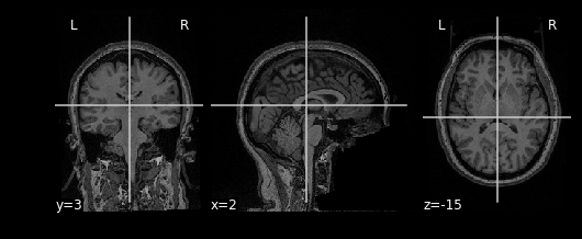
This gives just a still image of the brain. We can also view the
brain more interactively using the view_img function. It
will require some additional settings however:
PYTHON
nplot.view_img(t1_img,
               bg_img=False, # Disable using a standard image as the background
               cmap='Greys_r', # Set color scale so white matter appears lighter than grey
               symmetric_cmap=False, # We don't have negative values
               threshold="auto", # Clears out the background
              )
Try clicking and dragging the image in each of the views that are generated!
Try viewing the mask as well!
Arithmetic Operations
Let’s start performing some image operations. The simplest operations we can perform is element-wise, what this means is that we want to perform some sort of mathematical operation on each voxel of the MR image. Since voxels are represented in a 3D array, this is equivalent to performing an operation on each element (i,j,k) of a 3D array. Let’s try inverting the image, that is, flip the colour scale such that all blacks appear white and vice-versa. To do this, we’ll use the method
nimg.math_img(formula, **imgs) Where:
-
formulais a mathematical expression such as'a+1' -
**imgsis a set of key-value pairs linking variable names to images. For examplea=T1
In order to invert the image, we can simply flip the sign which will set the most positive elements (white) to the most negatve elements (black), and the least positives elements (black) to the least negative elements (white). This effectively flips the colour-scale:
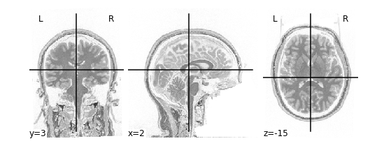
Alternatively we don’t need to first load in our
t1_imgusingimg.load_img. Instead we can feed in a path toimg.math_img:
invert_img = nimg.math_img('-a', a=t1)
nplot.plot_anat(invert_img)
This will yield the same result!
Applying a Mask
Let’s extend this idea of applying operations to each element of an image to multiple images. Instead of specifying just one image like the following:
nimg.math_img('a+1',a=img_a)
We can specify multiple images by tacking on additional variables:
nimg.math_img('a+b', a=img_a, b=img_b)
The key requirement here is that when dealing with multiple images,
that the size of the images must be the same. The reason being
is that we’re deaing with element-wise operations. That
means that some voxel (i,j,k) in img_a is being paired with
some voxel (i,j,k) in img_b when performing operations. So
every voxel in img_a must have some pair with a voxel in
img_b; sizes must be the same.
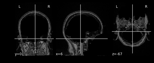
We can take advantage of this property when masking our data using
multiplication. Masking works by multipling a raw image (our
T1), with some mask image (our bm). Whichever
voxel (i,j,k) has a value of 0 in the mask multiplies with voxel (i,j,k)
in the raw image resulting in a product of 0. Conversely, any voxel
(i,j,k) in the mask with a value of 1 multiplies with voxel (i,j,k) in
the raw image resulting in the same value. Let’s try this out in
practice and see what the result is:

As you can see areas where the mask image had a value of 1 were retained, everything else was set to 0
Exercise #1
Try applying the mask such that the brain is removed, but the rest of the head is intact! Hint: Remember that a mask is composed of 0’s and 1’s, where parts of the data labelled 1 are regions to keep, and parts of the data that are 0, are to throw away. You can do this in 2 steps:
- Switch the 0’s and 1’s using an equation (simple addition/substraction) or condition (like x == 0).
- Apply the mask
Slicing
Recall that our data matrix is organized in the following manner:
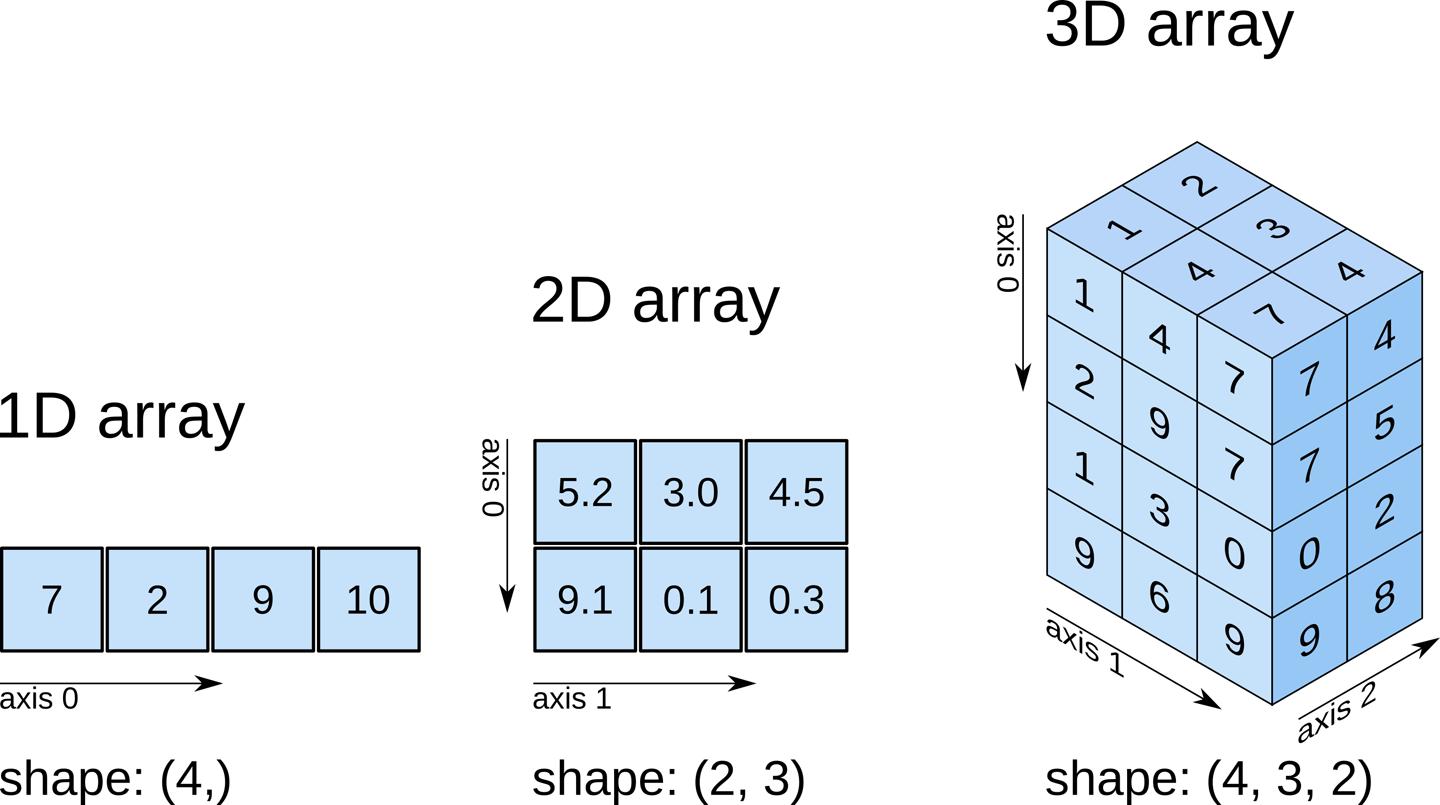
Slicing does exactly what it seems to imply. Given our 3D volume, we can pull out 2D subsets (called “slices”). Here’s an example of slicing moving from left to right via an animated GIF:
What you see here is a series of 2D images that start from the left, and move toward the right. Each frame of this GIF is a slice - a 2D subset of a 3D volume. Slicing can be useful for cases in which you’d want to loop through each MR slice and perform a computation; importantly in functional imaging data slicing is useful for pulling out timepoints as we’ll see later!
.gif)
Slicing is done easily on an image file using the attribute
.slicer of a Nilearn image object. For example
we can grab the \(10^{\text{th}}\)
slice along the x axis as follows:
The statement \(10:11\) is
intentional and is required by .slicer. Alternatively we
can slice along the x-axis using the data matrix itself:
This will yield the same result as above. Notice that when using the
t1_data array we can just specify which slice to grab
instead of using :. We can use slicing in order to modify
visualizations. For example, when viewing the T1 image, we may want to
specify at which slice we’d like to view the image. This can be done by
specifying which coordinates to cut the image at:
The cut_coords option specifies 3 numbers:
- The first number says cut the X coordinate at slice 50 and display (sagittal view in this case!)
- The second number says cut the Y coordinate at slice 30 and display (coronal view)
- The third number says cut the Z coordinate at slice 20 and display (axial view)
Remember nplot.plot_anat yields 3 images, therefore
cut_coords allows you to display where to take
cross-sections of the brain from different perspectives (axial,
sagittal, coronal)
This covers the basics of image manipulation using T1 images. To review in this section we covered:
- Basic image arithmetic
- Visualization
- Slicing
In the next section we will cover how to integrate additional
modalities (functional data) to what we’ve done so far using
Nilearn. Then we can start using what we’ve learned in
order to perform analysis and visualization!
- MR images are essentially 3D arrays where each voxel is represented by an (i,j,k) index
- Nilearn is Nibabel under the hood, knowing how Nibabel works is key to understanding Nilearn