Probabilistic tractography

Overview

Questions

• Why do we need tractography algorithms beyond the deterministic ones?
• How is probabilistic tractography different from deterministic tractography?

Objectives

• Understand the principles behind a probabilistic tractography algorithm
• Understand the aspects involved when analyzing the tractogram computed using a probabilistic algorithm

Probabilistic tractography

---

Probabilistic fiber tracking is a way of reconstructing the white matter structural connectivity using diffusion MRI data. Much like deterministic fiber tracking, the probabilistic approach follows the trajectory of a possible pathway in a step-wise fashion and propagate streamlines based on the local orientations reconstructed at each voxel.

In probabilistic tracking, however, the tracking direction at each point along the path is chosen at random from a distribution of possible directions, and thus is no longer deterministic. The distribution at each point is different and depends on the observed diffusion data at that point. The distribution of tracking directions at each point can be represented as a probability mass function (PMF) if the possible tracking directions are restricted to a set of points distributed on a sphere.

Like their deterministic counterparts, probabilistic tracking methods start propagating streamlines from a seed map, which contains a number of coordinates per voxel to initiate the procedure. The higher the number of seeds per voxel (i.e. the seed density), the larger the number of potentially recovered long-range connections. However, this comes at the cost of a longer running time.

This episode builds on top of the results of the CSD local orientation reconstruction method presented in a previous episode.

We will first get the necessary diffusion data, and compute the local orientation information using the CSD method:

PYTHON

import os

import nibabel as nib
import numpy as np

from bids.layout import BIDSLayout

from dipy.core.gradients import gradient_table
from dipy.io.gradients import read_bvals_bvecs

dwi_layout = BIDSLayout('../../data/ds000221/derivatives/uncorrected_topup_eddy/', validate=False)
gradient_layout = BIDSLayout('../../data/ds000221/', validate=False)

subj = '010006'

dwi_fname = dwi_layout.get(subject=subj, suffix='dwi', extension='.nii.gz', return_type='file')[0]
bvec_fname = dwi_layout.get(subject=subj, extension='.eddy_rotated_bvecs', return_type='file')[0]
bval_fname = gradient_layout.get(subject=subj, suffix='dwi', extension='.bval', return_type='file')[0]

dwi_img = nib.load(dwi)
affine = dwi_img.affine

gt_bvals, gt_bvecs = read_bvals_bvecs(bval, bvec)
gtab = gradient_table(gt_bvals, gt_bvecs)

We will now create the seeding mask and the seeds using an estimate of the white matter tissue based on the FA values obtained from the diffusion tensor:

PYTHON

from dipy.reconst import dti
from dipy.segment.mask import median_otsu
from dipy.tracking import utils

dwi_data = dwi_img.get_fdata()
dwi_data, dwi_mask = median_otsu(dwi_data, vol_idx=[0], numpass=1)  # Specify the volume index to the b0 volumes

dti_model = dti.TensorModel(gtab)
dti_fit = dti_model.fit(dwi_data, mask=dwi_mask)  # This step may take a while

# Create the seeding mask
fa_img = dti_fit.fa
seed_mask = fa_img.copy()
seed_mask[seed_mask >= 0.2] = 1
seed_mask[seed_mask < 0.2] = 0

# Create the seeds
seeds = utils.seeds_from_mask(seed_mask, affine=affine, density=1)

We will now estimate the FRF and set the CSD model to feed the local orientation information to the streamline propagation object:

PYTHON

from dipy.reconst.csdeconv import (ConstrainedSphericalDeconvModel,
                                   auto_response_ssst)

response, ratio = auto_response_ssst(gtab, dwi_data, roi_radii=10, fa_thr=0.7)
sh_order = 2
csd_model = ConstrainedSphericalDeconvModel(gtab, response, sh_order=sh_order)
csd_fit = csd_model.fit(dwi_data, mask=seed_mask)

Tracking methods are provided with a criterion to stop propagating streamlines beyond non-white matter tissues. One way to do this is to use the Generalized Fractional Anisotropy (GFA). Much like the Fractional Anisotropy issued by the DTI model measures anisotropy, the GFA uses samples of the ODF to quantify the anisotropy of tissues, and hence, it provides an estimation of the underlying tissue type.

PYTHON

from scipy import ndimage  # To rotate image for visualization purposes
import matplotlib.pyplot as plt
from dipy.reconst.shm import CsaOdfModel
from dipy.tracking.stopping_criterion import ThresholdStoppingCriterion

csa_model = CsaOdfModel(gtab, sh_order=sh_order)
gfa = csa_model.fit(dwi_data, mask=seed_mask).gfa
stopping_criterion = ThresholdStoppingCriterion(gfa, .2)

# Create the directory to save the results
out_dir = '../../data/ds000221/derivatives/dwi/tractography/sub-%s/ses-01/dwi/' % subj

if not os.path.exists(out_dir):
    os.makedirs(out_dir)

# Save the GFA
gfa_img = nib.Nifti1Image(gfa.astype(np.float32), affine)
nib.save(gfa_img, os.path.join(out_dir, 'gfa.nii.gz'))

# Plot the GFA
%matplotlib inline

fig, ax = plt.subplots(1, 3, figsize=(10, 10))
ax[0].imshow(ndimage.rotate(gfa[:, gfa.shape[1]//2, :], 90, reshape=False))
ax[1].imshow(ndimage.rotate(gfa[gfa.shape[0]//2, :, :], 90, reshape=False))
ax[2].imshow(ndimage.rotate(gfa[:, :, gfa.shape[-1]//2], 90, reshape=False))
fig.savefig(os.path.join(out_dir, "gfa.png"), dpi=300, bbox_inches="tight")
plt.show()

The GFA threshold stopping criterion value must be adjusted to the data in order to avoid creating a mask that will exclude white matter areas (which would result in streamlines being unable to propagate to other white matter areas). Visually inspecting the GFA map might provide with a sufficient guarantee about the goodness of the value.

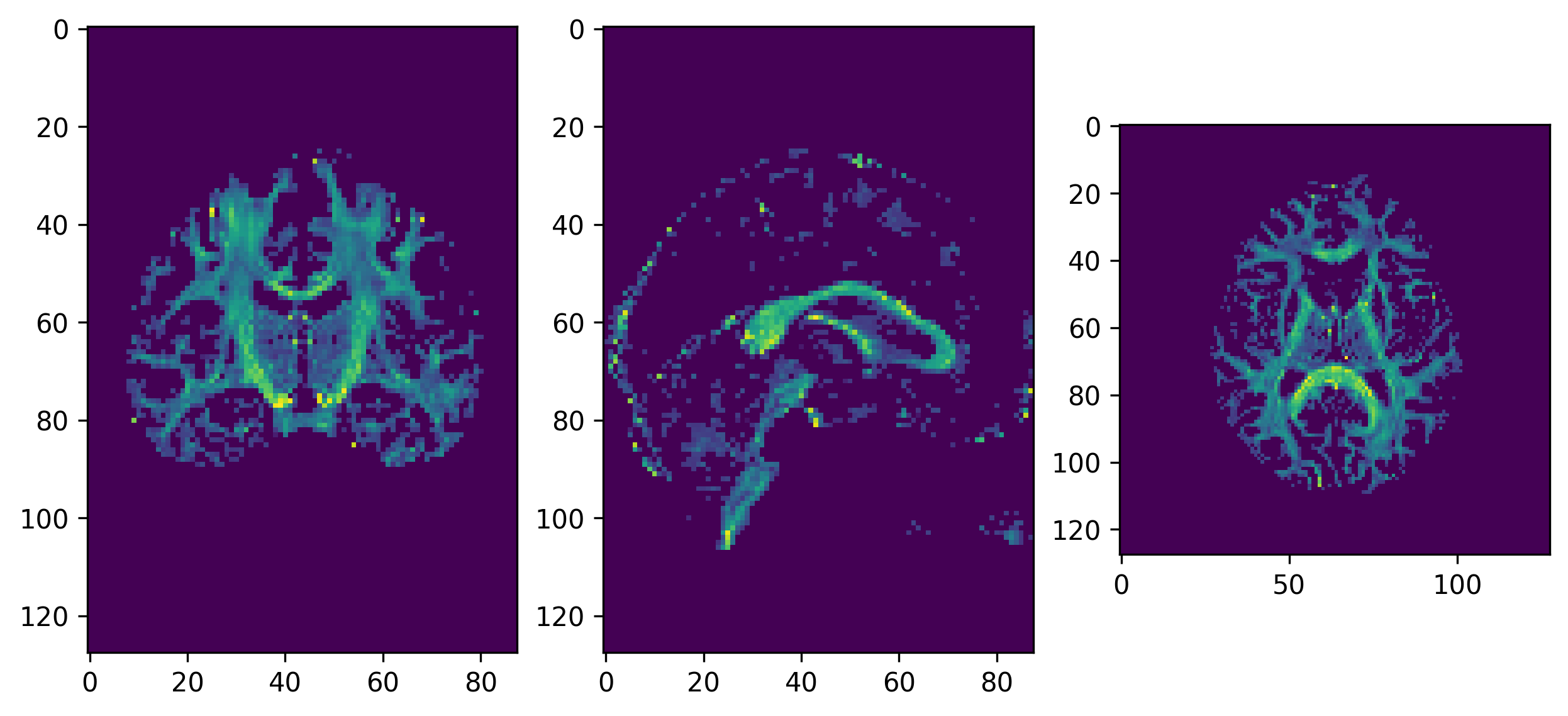
GFA

The Fiber Orientation Distribution (FOD) of the CSD model estimates the distribution of small fiber bundles within each voxel. We can use this distribution for probabilistic fiber tracking. One way to do this is to represent the FOD using a discrete sphere. This discrete FOD can be used by the ProbabilisticDirectionGetter as a PMF for sampling tracking directions. We need to clip the FOD to use it as a PMF because the latter cannot have negative values. Ideally, the FOD should be strictly positive, but because of noise and/or model failures sometimes it can have negative values.

The set of possible directions to choose to propagate a streamline is restricted by a cone angle \(\theta\), named max_angle in DIPY’s ProbabilisticDirectionGetter::from_pmf method.

Another relevant parameter of the propagation is the step size, which dictates how much the propagation will advance to the next point. Note that it is a real number, since the tracking procedure operates in physical coordinates.

Note that the LocalTracking class accepts a StoppingCriterion class instance as its second argument, and thus a different criterion can be used if the GFA criterion does not fit into our framework, or if different data is available in our workflow.

PYTHON

from dipy.direction import ProbabilisticDirectionGetter
from dipy.data import small_sphere
from dipy.io.stateful_tractogram import Space, StatefulTractogram
from dipy.io.streamline import save_tractogram
from dipy.tracking.local_tracking import LocalTracking
from dipy.tracking.streamline import Streamlines

fod = csd_fit.odf(small_sphere)
pmf = fod.clip(min=0)
prob_dg = ProbabilisticDirectionGetter.from_pmf(pmf, max_angle=30.,
                                                sphere=small_sphere)
streamline_generator = LocalTracking(prob_dg, stopping_criterion, seeds,
                                     affine, step_size=.5)
streamlines = Streamlines(streamline_generator)
sft = StatefulTractogram(streamlines, dwi_img, Space.RASMM)

# Save the tractogram
save_tractogram(sft, "tractogram_probabilistic_dg_pmf.trk")

We will easily generate the anatomical views on the generated tractogram using the generate_anatomical_volume_figure helper function:

PYTHON

from fury import actor, colormap

from utils.visualization_utils import generate_anatomical_volume_figure

# Plot the tractogram

# Build the representation of the data
streamlines_actor = actor.line(streamlines, colormap.line_colors(streamlines))

# Generate the figure
fig = generate_anatomical_volume_figure(streamlines_actor)

fig.savefig(os.path.join(out_dir, "tractogram_probabilistic_dg_pmf.png"),
            dpi=300, bbox_inches="tight")
plt.show()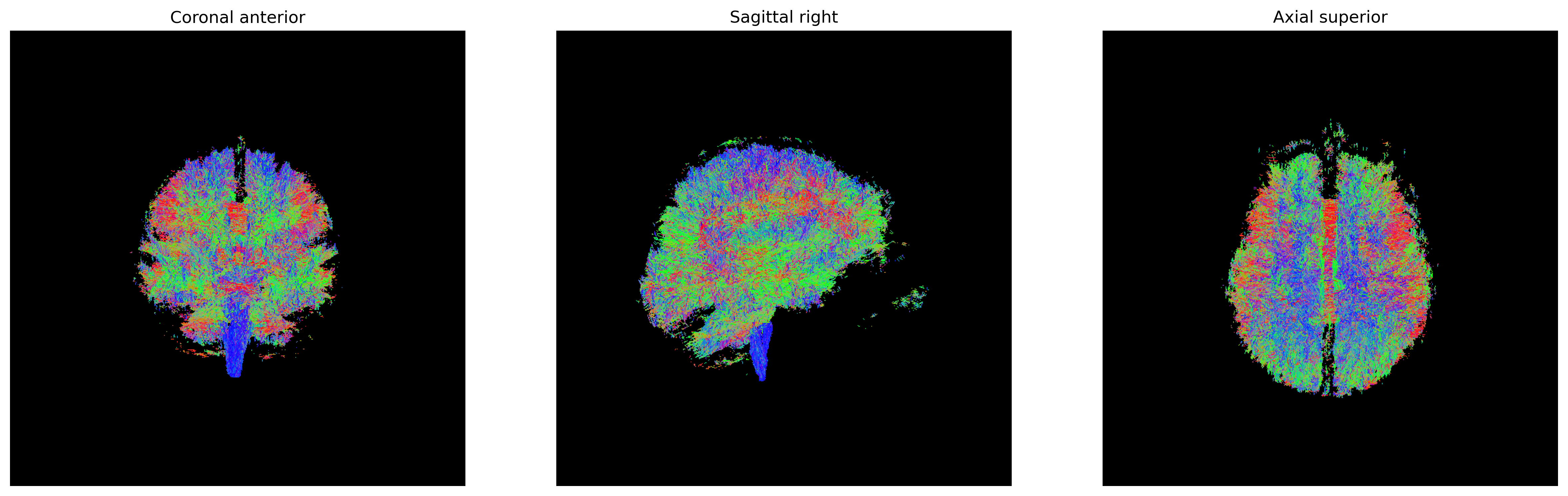

Streamlines representing white matter using probabilistic direction getter from PMF

One disadvantage of using a discrete PMF to represent possible tracking directions is that it tends to take up a lot of RAM memory. The size of the PMF, the FOD in this case, must be equal to the number of possible tracking directions on the hemisphere, and every voxel has a unique PMF. In this case the data is (81, 106, 76) and small_sphere has 181 directions so the FOD is (81, 106, 76, 181). One way to avoid sampling the PMF and holding it in memory is to build the direction getter directly from the spherical harmonic (SH) representation of the FOD. By using this approach, we can also use a larger sphere, like default_sphere which has 362 directions on the hemisphere, without having to worry about memory limitations.

PYTHON

from dipy.data import default_sphere

prob_dg = ProbabilisticDirectionGetter.from_shcoeff(csd_fit.shm_coeff,
                                                    max_angle=30.,
                                                    sphere=default_sphere)
streamline_generator = LocalTracking(prob_dg, stopping_criterion, seeds,
                                     affine, step_size=.5)
streamlines = Streamlines(streamline_generator)
sft = StatefulTractogram(streamlines, dwi_img, Space.RASMM)

# Save the tractogram
save_tractogram(sft, "tractogram_probabilistic_dg_sh.trk")

We will visualize the tractogram using the three usual anatomical views:

PYTHON

# Plot the tractogram

# Build the representation of the data
streamlines_actor = actor.line(streamlines, colormap.line_colors(streamlines))

# Generate the figure
fig = generate_anatomical_volume_figure(streamlines_actor)

fig.savefig(os.path.join(out_dir, "tractogram_probabilistic_dg_sh.png"),
            dpi=300, bbox_inches="tight")
plt.show()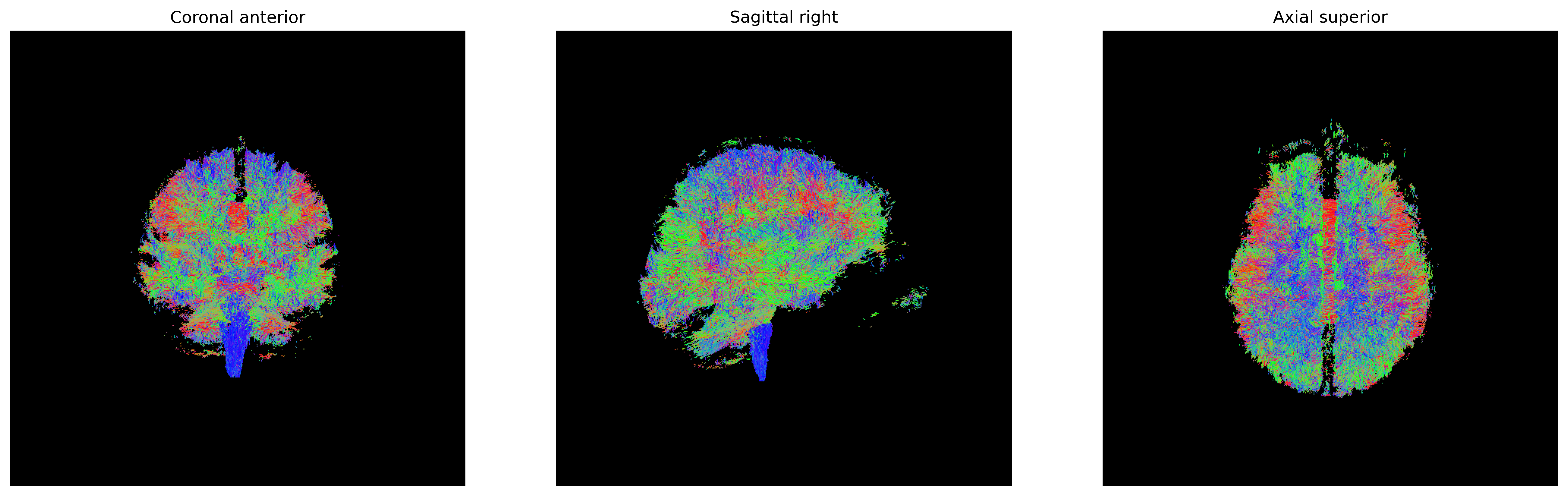

Streamlines representing white matter using probabilistic direction getter from SH

Not all model fits have the shm_coeff attribute because not all models use this basis to represent the data internally. However we can fit the ODF of any model to the spherical harmonic basis using the peaks_from_model function.

PYTHON

from dipy.direction import peaks_from_model

peaks = peaks_from_model(csd_model, dwi_data, default_sphere, .5, 25,
                         mask=seed_mask, return_sh=True, parallel=True)

It is always good practice to (save and) visualize the peaks as a check towards ensuring that the orientation information conforms to what is expected as input to the tracking process.

PYTHON

# Save the peaks
nib.save(nib.Nifti1Image(reshape_peaks_for_visualization(peaks),
                         affine), os.path.join(out_dir, 'peaks.nii.gz'))

As usual, we will use FURY to visualize the peaks:

PYTHON

from utils.visualization_utils import generate_anatomical_slice_figure

# Visualize the peaks

# Build the representation of the data
peaks_actor = actor.peak_slicer(peaks.peak_dirs, peaks.peak_values)

# Compute the slices to be shown
slices = tuple(elem // 2 for elem in dwi_data.shape[:-1])

# Generate the figure
fig = generate_anatomical_slice_figure(slices, peaks_actor)

fig.savefig(os.path.join(out_dir, "peaks.png"), dpi=300, bbox_inches="tight")
plt.show()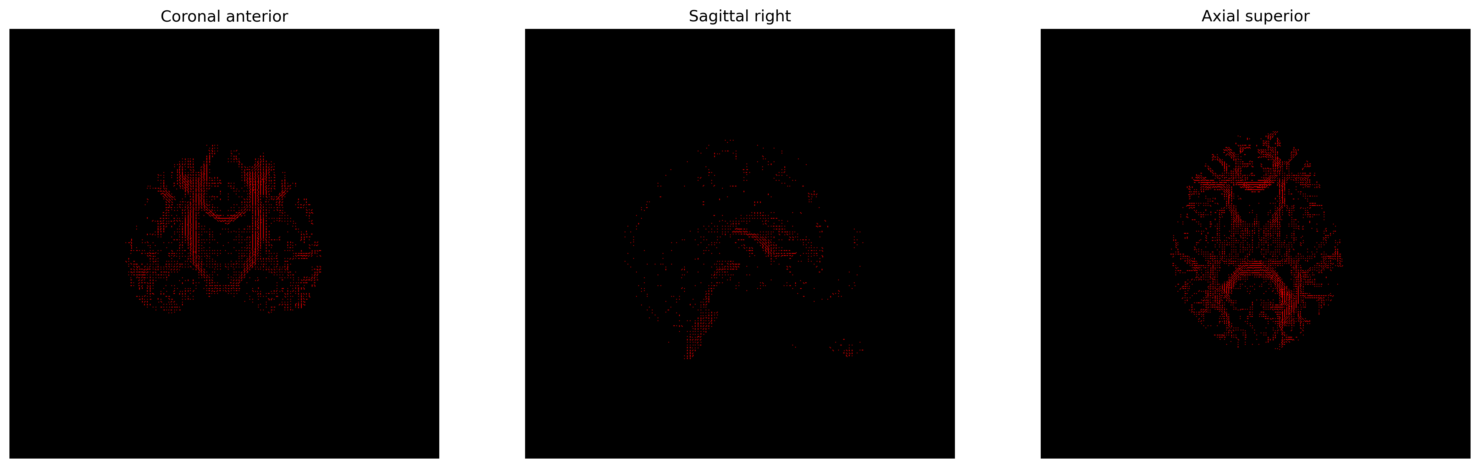

Peaks obtained from the CSD model for tracking purposes

We will now perform the tracking process using the local orientation information provided by the peaks:

PYTHON

fod_coeff = peaks.shm_coeff

prob_dg = ProbabilisticDirectionGetter.from_shcoeff(fod_coeff, max_angle=30.,
                                                    sphere=default_sphere)
streamline_generator = LocalTracking(prob_dg, stopping_criterion, seeds,
                                     affine, step_size=.5)
streamlines = Streamlines(streamline_generator)
sft = StatefulTractogram(streamlines, dwi_img, Space.RASMM)

# Save the tractogram
save_tractogram(sft, "tractogram_probabilistic_dg_sh_pmf.trk")

We will again visualize the tractogram using the three usual anatomical views:

PYTHON

# Plot the tractogram

# Build the representation of the data
streamlines_actor = actor.line(streamlines, colormap.line_colors(streamlines))

# Generate the figure
fig = generate_anatomical_volume_figure(streamlines_actor)

fig.savefig(os.path.join(out_dir, "tractogram_probabilistic_dg_sh_pmf.png"),
            dpi=300, bbox_inches="tight")
plt.show()

Streamlines representing white matter using probabilistic direction getter from SH (peaks_from_model)

Tip: Making sure your tractogram is well aligned with the data

If for whatever reason the anatomical and diffusion images were not correctly aligned, you may find that your tractogram is not well aligned with the anatomical data. This may also happen derived from the different formats in which a tractogram is saved/loaded, some conventions specifying the origin at the voxel corner and other specifying it at the center of the voxel. Visualizing the computed features is always recommended. There are some tools that allow to ensure that the matrices specifying the orientation and positioning of the data should be correct.

MRtrix’s mrinfo command can be used to visualize the affine matrix of a NIfTI file as:

BASH

mrinfo dwi.nii.gz

which would output something like:

OUTPUT

************************************************
Image:               "/data/dwi.nii.gz"
************************************************
  Dimensions:        90 x 108 x 90 x 33
  Voxel size:        2 x 2 x 2 x 1
  Data strides:      [ -1 -2 3 4 ]
  Format:            NIfTI-1.1 (GZip compressed)
  Data type:         signed 16 bit integer (little endian)
  Intensity scaling: offset = 0, multiplier = 1
  Transform:                    1          -0           0      -178
                               -0           1           0      -214
                               -0          -0           1        -0

Similarly, for your tractograms, you may use the command track_info from TrackVis’ Diffusion Toolkit set of command-line tools:

BASH

track_info tractogram.trk

which would output something like:

OUTPUT

ID string:            TRACK
Version:              2
Dimension:            180 216 180
Voxel size:           1 1 1
Voxel order:          LPS
Voxel order original: LPS
Voxel to RAS matrix:
     -1.0000     0.0000     0.0000     0.5000
      0.0000    -1.0000     0.0000     0.5000
      0.0000     0.0000     1.0000    -0.5000
      0.0000     0.0000     0.0000     1.0000

Image Orientation:  1.0000/0.0000/0.0000/0.0000/1.0000/0.0000
Orientation patches:  none
Number of scalars:  0
Number of properties: 0
Number of tracks: 200433

Note that, a TRK file contains orientational and positional information. If you choose to store your tractograms using the TCK format, this information will not be contained in the file. To see the file header information you may use the MRtrix tckinfo command:

BASH

tckinfo tractogram.tck

which would output something like:

OUTPUT

***********************************
 Tracks file: "/data/tractogram.tck"
   count:                0000200433
   dimensions:           (180, 216, 180)
   voxel_order:          LPS
   voxel_sizes:          (1.0, 1.0, 1.0)

Key Points

• Probabilistic tractography incorporates uncertainty to the tracking process
• Provides tractograms that explore more white matter axonal fibers