Deterministic tractography
Last updated on 2024-02-18 | Edit this page
Overview
Questions
- What computations does a deterministic tractography require?
- How can we visualize the streamlines generated by a tractography method?
Objectives
- Be able to perform deterministic tracking on diffusion MRI data
- Familiarize with the data entities of a tractogram
Deterministic tractography
Deterministic tractography algorithms perform tracking of streamlines by following a predictable path, such as following the primary diffusion direction.
In order to demonstrate how to perform deterministic tracking on a diffusion MRI dataset, we will build from the preprocessing presented in a previous episode and compute the diffusion tensor.
PYTHON
import os

import nibabel as nib
import numpy as np

from bids.layout import BIDSLayout

from dipy.io.gradients import read_bvals_bvecs
from dipy.core.gradients import gradient_table

dwi_layout = BIDSLayout("../../data/ds000221/derivatives/uncorrected_topup_eddy", validate=False)
gradient_layout = BIDSLayout("../../data/ds000221/", validate=False)

subj = '010006'

dwi_fname = dwi_layout.get(subject=subj, suffix='dwi', extension='.nii.gz', return_type='file')[0]
bvec_fname = dwi_layout.get(subject=subj, extension='.eddy_rotated_bvecs', return_type='file')[0]
bval_fname = gradient_layout.get(subject=subj, suffix='dwi', extension='.bval', return_type='file')[0]

dwi_img = nib.load(dwi_fname)
affine = dwi_img.affine

bvals, bvecs = read_bvals_bvecs(bval_fname, bvec_fname)
gtab = gradient_table(bvals, bvecs)
We will now create a mask and constrain the fitting within the mask.
Tractography run times
Note that many steps in the streamline propagation procedure are computationally intensive, and thus may take a while to complete.
PYTHON
import dipy.reconst.dti as dti
from dipy.segment.mask import median_otsu

dwi_data = dwi_img.get_fdata()
dwi_data, dwi_mask = median_otsu(dwi_data, vol_idx=[0], numpass=1)  # Specify the volume index to the b0 volumes

dti_model = dti.TensorModel(gtab)
dti_fit = dti_model.fit(dwi_data, mask=dwi_mask)  # This step may take a while
We will perform tracking using a deterministic algorithm on tensor
fields via EuDX (Garyfallidis
et al., 2012). EuDX makes use of the primary
direction of the diffusion tensor to propagate streamlines from voxel to
voxel and a stopping criteria from the fractional anisotropy (FA).
We will first get the FA map and eigenvectors from our tensor
fitting. In the background of the FA map, the fitting may not be
accurate as all of the measured signal is primarily noise and it is
possible that values of NaNs (not a number) may be found in the FA map.
We can remove these using numpy to find and set these
voxels to 0.
PYTHON
# Create the directory to save the results

out_dir = f"../../data/ds000221/derivatives/dwi/tractography/sub-{subj}/ses-01/dwi/"

if not os.path.exists(out_dir):
    os.makedirs(out_dir)

fa_img = dti_fit.fa
evecs_img = dti_fit.evecs

fa_img[np.isnan(fa_img)] = 0

# Save the FA
fa_nii = nib.Nifti1Image(fa_img.astype(np.float32), affine)
nib.save(fa_nii, os.path.join(out_dir, 'fa.nii.gz'))

# Plot the FA
import matplotlib.pyplot as plt
from scipy import ndimage  # To rotate image for visualization purposes

%matplotlib inline

fig, ax = plt.subplots(1, 3, figsize=(10, 10))
ax[0].imshow(ndimage.rotate(fa_img[:, fa_img.shape[1]//2, :], 90, reshape=False))
ax[1].imshow(ndimage.rotate(fa_img[fa_img.shape[0]//2, :, :], 90, reshape=False))
ax[2].imshow(ndimage.rotate(fa_img[:, :, fa_img.shape[-1]//2], 90, reshape=False))
fig.savefig(os.path.join(out_dir, "fa.png"), dpi=300, bbox_inches="tight")
plt.show()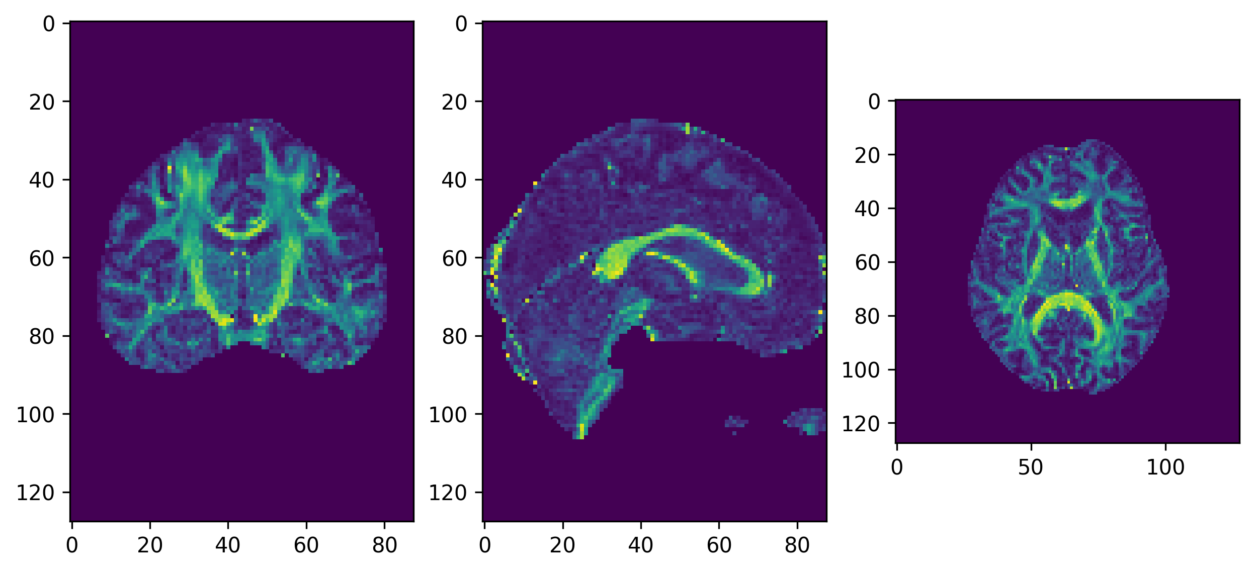
One of the inputs of EuDX is the discretized voxel
directions on a unit sphere. Therefore, it is necessary to discretize
the eigenvectors before providing them to EuDX. We will use
an evenly distributed sphere of 362 points using the
get_sphere function.
We will determine the indices representing the discretized directions of the peaks by providing as input, our tensor model, the diffusion data, the sphere, and a mask to apply the processing to. Additionally, we will set the minimum angle between directions, the maximum number of peaks to return (1 for the tensor model), and the relative peak threshold (returning peaks greater than this value).
PYTHON
from dipy.direction import peaks_from_model

peak_indices = peaks_from_model(
    model=dti_model, data=dwi_data, sphere=sphere, relative_peak_threshold=.2,
    min_separation_angle=25, mask=dwi_mask, npeaks=2)
Additionally, we will apply a stopping criterion for our tracking based on the FA map. That is, we will stop our tracking when we reach a voxel where FA is below 0.2.
PYTHON
from dipy.tracking.stopping_criterion import ThresholdStoppingCriterion

stopping_criterion = ThresholdStoppingCriterion(fa_img, .2)
We will also need to specify where to “seed” (begin) the fiber tracking. Generally, the seeds chosen will depend on the pathways one is interested in modelling. In this example, we will create a seed mask from the FA map thresholding above our stopping criterion.
PYTHON
from dipy.tracking import utils

seed_mask = fa_img.copy()
seed_mask[seed_mask >= 0.2] = 1
seed_mask[seed_mask < 0.2] = 0

seeds = utils.seeds_from_mask(seed_mask, affine=affine, density=1)
Now, we can apply the tracking algorithm!
As mentioned previously, EuDX is the fiber tracking
algorithm that we will be using. The most important parameters to
include are the indices representing the discretized directions of the
peaks (peak_indices), the stopping criterion, the seeds,
the affine transformation, and the step sizes to take when tracking!
PYTHON
from dipy.tracking.local_tracking import LocalTracking
from dipy.tracking.streamline import Streamlines

# Initialize local tracking - computation happens in the next step.
streamlines_generator = LocalTracking(
    peak_indices, stopping_criterion, seeds, affine=affine, step_size=.5)

# Generate streamlines object
streamlines = Streamlines(streamlines_generator)
We just created a deterministic set of streamlines using the
EuDX algorithm mapping the human brain connectome
(tractography). We can save the streamlines as a Trackvis
file so it can be loaded into other software for visualization or
further analysis. To do so, we need to save the tractogram state using
StatefulTractogram and save_tractogram to save
the file. Note that we will have to specify the space to save the
tractogram in.
PYTHON
from dipy.io.stateful_tractogram import Space, StatefulTractogram
from dipy.io.streamline import save_tractogram

sft = StatefulTractogram(streamlines, dwi_img, Space.RASMM)

# Save the tractogram
save_tractogram(sft, os.path.join(out_dir, "tractogram_deterministic_EuDX.trk"))
We can then generate the streamlines 3D scene using the
FURY python package, and visualize the scene’s contents
with Matplotlib.
PYTHON
from fury import actor, colormap

from utils.visualization_utils import generate_anatomical_volume_figure

# Plot the tractogram

# Build the representation of the data
streamlines_actor = actor.line(streamlines, colormap.line_colors(streamlines))

# Generate the figure
fig = generate_anatomical_volume_figure(streamlines_actor)

fig.savefig(os.path.join(out_dir, "tractogram_deterministic_EuDX.png"),
            dpi=300, bbox_inches="tight")
plt.show()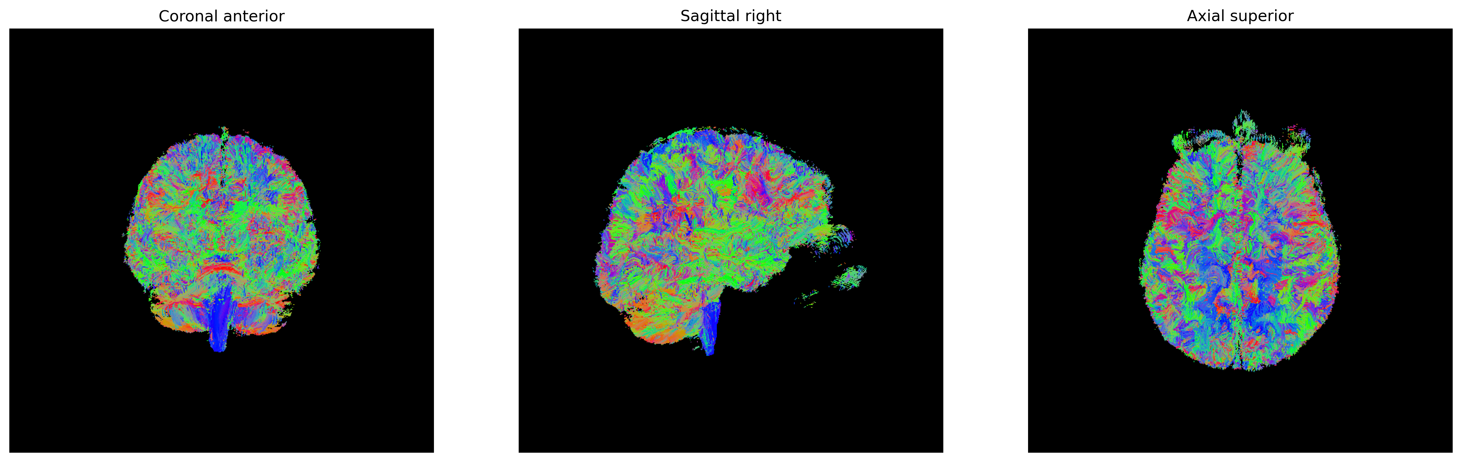
Exercise 1
In this episode, we applied a threshold stopping criteria to stop
tracking when we reach a voxel where FA is below 0.2. There are also
other stopping criteria available. We encourage you to read the
DIPY documentation about the others. For this exercise,
repeat the tractography, but apply a binary stopping criteria
(BinaryStoppingCriterion) using the seed mask. Visualize
the tractogram!
PYTHON
import os

import nibabel as nib
import numpy as np

from bids.layout import BIDSLayout

from dipy.io.gradients import read_bvals_bvecs
from dipy.core.gradients import gradient_table
from dipy.data import get_sphere
from dipy.direction import peaks_from_model
import dipy.reconst.dti as dti
from dipy.segment.mask import median_otsu
from dipy.tracking import utils
from dipy.tracking.local_tracking import LocalTracking
from dipy.tracking.streamline import Streamlines

from utils.visualization_utils import generate_anatomical_volume_figure
from fury import actor, colormap
import matplotlib.pyplot as plt

dwi_layout = BIDSLayout("../../data/ds000221/derivatives/uncorrected_topup_eddy", validate=False)
gradient_layout = BIDSLayout("../../data/ds000221/", > > validate=False)

# Get subject data
subj = '010006'
dwi_fname = dwi_layout.get(subject=subj, suffix='dwi', extension='.nii.gz', return_type='file')[0]
bvec_fname = dwi_layout.get(subject=subj, extension='.eddy_rotated_bvecs', return_type='file')[0]
bval_fname = gradient_layout.get(subject=subj, suffix='dwi', extension='.bval', return_type='file')[0]

dwi_img = nib.load(dwi_fname)
affine = dwi_img.affine

bvals, bvecs = read_bvals_bvecs(bval_fname, bvec_fname)
gtab = gradient_table(bvals, bvecs)

dwi_data = dwi_img.get_fdata()
dwi_data, dwi_mask = median_otsu(dwi_data, vol_idx=[0], numpass=1)  # Specify the volume index to the b0 volumes

# Fit tensor and compute FA map
dti_model = dti.TensorModel(gtab)
dti_fit = dti_model.fit(dwi_data, mask=dwi_mask)
fa_img = dti_fit.fa
evecs_img = dti_fit.evecs

sphere = get_sphere('symmetric362')
peak_indices = peaks_from_model(
       model=dti_model, data=dwi_data, sphere=sphere,
       relative_peak_threshold=.2, min_separation_angle=25, mask=dwi_mask,
       npeaks=2)

# Create a binary seed mask
seed_mask = fa_img.copy()
seed_mask[seed_mask >= 0.2] = 1
seed_mask[seed_mask < 0.2] = 0

seeds = utils.seeds_from_mask(seed_mask, affine=affine, density=1)

# Set stopping criteria
stopping_criterion = BinaryStoppingCriterion(seed_mask==1)

# Perform tracking
streamlines_generator = LocalTracking(
    peak_indices, stopping_criterion, seeds, affine=affine, step_size=.5)
streamlines = Streamlines(streamlines_generator)

# Plot the tractogram
# Build the representation of the data
streamlines_actor = actor.line(streamlines, colormap.line_colors(streamlines))

# Generate the figure
fig = generate_anatomical_volume_figure(streamlines_actor)
plt.show()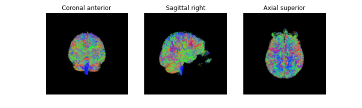
Exercise 2
As an additional challenge, set the color of the streamlines to
display the values of the FA map and change the opacity to
0.05. You may need to transform the streamlines from world
coordinates to the subject’s native space using
transform_streamlines from
dipy.tracking.streamline.
PYTHON
import numpy as np
from fury import actor

from dipy.tracking.streamline import transform_streamlines
from utils.visualizations_utils import generate_anatomical_volume_figure
import matplotlib.pyplot as plt

streamlines_native = transform_streamlines(streamlines, np.linalg.inv(affine))
streamlines_actor = actor.line(streamlines_native, fa_img, opacity=0.05)

fig = generate_anatomical_volume_figure(streamlines_actor)
plt.show()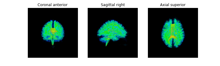
- Deterministic tractography methods perform tracking in a predictable way