Identify the problem and make a plan
Last updated on 2024-12-03 | Edit this page
Overview
Questions
- What do I do when I encounter an error?
- What do I do when my code outputs something I don’t expect?
- Why do errors and warnings appear in R?
- Which areas of code are responsible for errors?
- How can I fix my code? What other options exist if I can’t fix it?
Objectives
After completing this episode, participants should be able to…
- decode/describe what an error message is trying to communicate
- Identify specific lines and/or functions generating the error message
- Lookup function syntax, use, and examples using R Documentation (?help calls)
- Describe a general category of error message (e.g. syntax error, semantic errors, package-specific errors, etc.) # be more explicit about semantic errors?
- Describe the output of code you are seeking. ## identify relevant warnings or code output
- Identify and quickly fix commonly-encountered R errors ###### what was I thinking here
- Identify which problems are better suited for asking for further help, including online help and reprex
R
library(readr)
library(dplyr)
OUTPUT
Attaching package: 'dplyr'OUTPUT
The following objects are masked from 'package:stats':

    filter, lag
OUTPUT
The following objects are masked from 'package:base':

    intersect, setdiff, setequal, union
R
library(ggplot2)
library(stringr)

# Read in the data
rodents <- read_csv("data/surveys_complete_77_89.csv")
OUTPUT
Rows: 16878 Columns: 13OUTPUT
── Column specification ────────────────────────────────────────────────────────
Delimiter: ","
chr (6): species_id, sex, genus, species, taxa, plot_type
dbl (7): record_id, month, day, year, plot_id, hindfoot_length, weight

ℹ Use `spec()` to retrieve the full column specification for this data.
ℹ Specify the column types or set `show_col_types = FALSE` to quiet this message.
As simple as it may seem, the first step we’ll cover is what to do when encountering an error or other undesired output from your code. It is our experience that many seemingly-impossible errors can be fixed on the route to create a reproducible example for an expert helper. With this episode, we hope to teach you the basics about identifying how your error might be occurring, and how to isolate the problem for others to look at.
3.1 What do I do when I encounter an error?
Something that may go wrong is an error in your code. By this, we mean any code which generates an error message. This happens when R is unable to run your code, for a variety of reasons: some common ones include R being unable to read or interpret your commands, expecting different input types than those inputted, and user-written errors from checks you or other package creators have added to ensure your code is running correctly.
The accompanying error message attempts to tell you exactly how your code failed. For example, consider the following error message that occurs when I run this command in the R console:
R
ggplot(x = taxa) + geom_bar()
ERROR
Error: object 'taxa' not foundThough we know somewhere there is an object called taxa
(it is actually a column of the dataset rodents), R is
trying to communicate that it cannot find any such object in the local
environment. Let’s try again, appropriately pointing ggplot to the
rodents dataset and taxa column using the
$ operator.
R
ggplot(aes(x = rodents$taxa)) + geom_bar()
ERROR
Error in `fortify()` at ggplot2/R/plot.R:121:3:
! `data` must be a <data.frame>, or an object coercible by `fortify()`,
  or a valid <data.frame>-like object coercible by `as.data.frame()`, not a
  <uneval> object.
ℹ Did you accidentally pass `aes()` to the `data` argument?
Whoops! Here we see another error message – this time, R responds with a perhaps more-uninterpretable message.
Let’s go over each part briefly. First, we see an error from a
function called fortify, which we didn’t even call! Then a
much more helpful informational message: Did we accidentally pass
aes() to the data argument? This does seem to
relate to our function call, as we do pass aes, potentially
where our data should go. A helpful starting place when attempting to
decipher an error message is checking the documentation for the function
which caused the error:
?ggplot
Here, a Help window pops up in RStudio which provides some more
information. Skipping the general description at the top, we see ggplot
takes positional arguments of data, then
mapping, which uses the aes call. We can see
in “Arguments” that the aes(x = rodents$taxa) object used
in the plot is attempted by fortify to be converted to a
data.frame: now the picture is clear! We accidentally passed our
mapping argument (telling ggplot how to map variables to
the plot) into the position it expected data in the form of
a data frame. And if we scroll down to “Examples”, to “Pattern 1”, we
can see exactly how ggplot expects these arguments in practice. Let’s
amend our result:
R
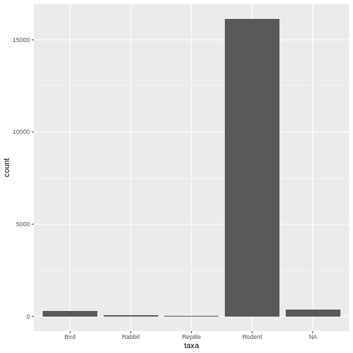
ggplot(rodents, aes(x = taxa)) + geom_bar()

Here we see our desired plot.
Summary
In general, when encountering an error message for which a remedy is not immediately apparent, some steps to take include:
Reading each part of the error message, to see if we can interpret and act on any.
Pulling up the R Documentation for that function (which may be specific to a package, such as with ggplot).
Reading through the documentation’s Description, Usage, Arguments, Details and Examples entries for greater insight into our error.
Copying and pasting the error message into a search engine for more interpretable explanations.
And, when all else fails, preparing our code into a reproducible example for expert help.
3.2 What do I do when my code outputs something I don’t expect
Another type of ‘error’ which you may encounter is when your R code runs without errors, but does not produce the desired output. You may sometimes see these called “semantic errors” (as opposed to syntax errors, though these term themselves are vague within computer science and describe a variety of different scenarios). As with actual R errors, semantic errors may occur for a variety of non-intuitive reasons, and are often harder to solve as there is no description of the error – you must work out where your code is defective yourself!
With our rodent analysis, the next step in the plan is to subset to
just the Rodent taxa (as opposed to other taxa: Bird,
Rabbit, Reptile or NA). Let’s quickly check to see how much data we’d be
throwing out by doing so:
R
table(rodents$taxa)
OUTPUT
   Bird  Rabbit Reptile  Rodent
    300      69       4   16148
We’re interested in the Rodents, and thankfully it seems like a majority of our observations will be maintained when subsetting to rodents. Except wait. In our plot, we can clearly see the presence of NA values. Why are we not seeing them here? This is an example of a semantic error – our command is executed correctly, but the output is not everything we intended. Having no error message to interpret, let’s jump straight to the documentation:
R
?table
OUTPUT
Help on topic 'table' was found in the following packages:

  Package               Library
  vctrs                 /home/runner/.local/share/renv/cache/v5/linux-ubuntu-jammy/R-4.4/x86_64-pc-linux-gnu/vctrs/0.6.5/c03fa420630029418f7e6da3667aac4a
  base                  /home/runner/.cache/R/renv/sandbox/linux-ubuntu-jammy/R-4.4/x86_64-pc-linux-gnu/9a444a72


Using the first match ...
Here, the documentation provides some clues: there seems to be an
argument called useNA that accepts “no”, “ifany”, and
“always”, but it’s not immediately apparent which one we should use. As
a second approach, let’s go to Examples to see if we can
find any quick fixes. Here we see a couple lines further down:
R
table(a)                 # does not report NA's
table(a, exclude = NULL) # reports NA's
That seems like it should be inclusive. Let’s try again:
R
table(rodents$taxa, exclude = NULL)
OUTPUT
   Bird  Rabbit Reptile  Rodent    <NA>
    300      69       4   16148     357
Now, we do see that by subsetting to the “Rodent” taxa, we are losing about 357 NAs, which themselves could be rodents! However, in this case, it seems a small enough portion to safely omit. Let’s subset our data to the rodent taxa
R
rodents <- rodents %>% filter(taxa == "Rodent")
Summary
In general, when encountering a semantic error for which a remedy is not immediately apparent, some steps to take include:
Reading any warning or informational messages that may pop up when executing your code.
Changing the input to your function call to see if the behavior is …
Pulling up the R Documentation for that function (which may be specific to a package, such as with ggplot).
Reading through the documentation’s Description, Usage, Arguments, Details and Examples entries for greater insight into our error.
And, when all else fails, preparing our code into a reproducible example for expert help. Note, there are fewer options available as when an error message prevents your code from running. You may find yourself isolating and reproducing your problem more often with semantic errors as easily solvable syntax errors.
Callout
Generally, the more your code deviates from just using base R
functions, or the more you use specific packages, both the quality of
documentation and online help available from search engines and Googling
gets worse and worse. While base R errors will often be solvable in a
couple of minutes from a quick ?help check or a long online
discussion and solutions on a website like Stack Overflow, errors
arising from little-used packages applied in bespoke analyses might
merit isolating your specific problem to a reproducible example for
online help, or even getting in touch with the developers! Such
community input and questions are often the way packages and
documentation improves over time.
3.3 How can I find where my code is failing?
Isolating your problem may not be as simple as assessing the output from a single function call on the line of code which produces your error. Often, it may be difficult to determine which line(s) in your code are producing the error.
Consider the example below, where we now are attempting to see how which species of kangaroo rodents appear in different plot types over the years.
R
krats <- rodents %>% filter(genus == "Dipadomys") #kangaroo rat genus

ggplot(krats, aes(year, fill=plot_type)) +
geom_histogram() +
facet_wrap(~species)
ERROR
Error in `combine_vars()` at ggplot2/R/facet-wrap.R:186:5:
! Faceting variables must have at least one value.
Uh-oh. Another error here, this time in “combine_vars?” What is that? “Faceting variables must have at least one value”: What does that mean?
Well it may be clear enough that we seem to be missing “species” values where we intend. Maybe we can try to make a different graph looking at what species values are present? Or perhaps there’s an error earlier – our safest approach may actually be seeing what krats looks like:
R
krats
OUTPUT
# A tibble: 0 × 13
# ℹ 13 variables: record_id <dbl>, month <dbl>, day <dbl>, year <dbl>,
#   plot_id <dbl>, species_id <chr>, sex <chr>, hindfoot_length <dbl>,
#   weight <dbl>, genus <chr>, species <chr>, taxa <chr>, plot_type <chr>
It’s empty! What went wrong with our “Dipadomys” filter?
R
rodents %>% count(genus)
OUTPUT
# A tibble: 12 × 2
   genus                n
   <chr>            <int>
 1 Ammospermophilus   136
 2 Baiomys              3
 3 Chaetodipus        382
 4 Dipodomys         9573
 5 Neotoma            904
 6 Onychomys         1656
 7 Perognathus        553
 8 Peromyscus        1271
 9 Reithrodontomys   1412
10 Rodent               4
11 Sigmodon           103
12 Spermophilus       151
We see two things here. For one, we’ve misspelled Dipodomys, which we can now amend. This quick function call also tells us we should expect a data frame with 9573 values resulting after subsetting to the genus Dipodomys.
R
krats <- rodents %>% filter(genus == "Dipodomys") #kangaroo rat genus
dim(krats)
OUTPUT
[1] 9573 13R
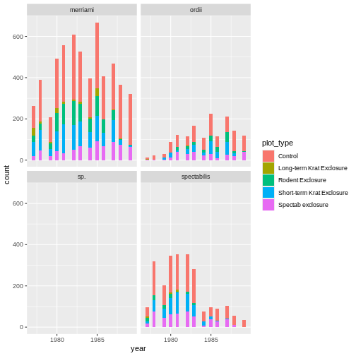
ggplot(krats, aes(year, fill=plot_type)) +
geom_histogram() +
facet_wrap(~species)
OUTPUT
`stat_bin()` using `bins = 30`. Pick better value with `binwidth`.
Our improved code here looks good. A quick “dim” call confirms we now have all the Dipodomys observations, and our plot is looking better. In general, having a ‘print’ statement or some other output before plots or other major steps can be a good way to check your code is producing intermediate results consistent with your expectations.
However, there’s something funky happening here. The bins are definitely weirdly spaced – we can see some bins are not filled with any observations, while those exactly containing one of the integer years happens to contain all the observations for that year.
Challenge
As a group, name some potential problems or undesired outcomes from this graph…
- The graph looks sparse, and unevenly so – many bins have no observations
- Suggests that some years had more observations and others fewer based on somewhat arbitrary measurements (i.e. what calendar year happened to fall on)
- Hard to compare trends across time, or even subsequent years…
As we discussed in the challenge, there are some issues to visualizing our data this way. A solution here might be to tinker with the bin width in the histogram code, but let’s step back a minute. Do we necessarily need to dive into the depths of tinkering with the plot? We can evalulate this problem not in terms of the plot having a problem, but with our data type having a problem. There’s an opportunity to encode the observation times outside of coarse, somewhat arbitrary year groupings with the real, interpretable date they were collected. Let’s do that using the tidyverse’s ‘lubridate’ package. The important details here are that we are creating a ‘datetime’-type variable using the recorded years, months, and days, which are currently all encoded as numeric types.
R
krats <- rodents %>% filter(genus == "Dipodomys") #kangaroo rat genus
dim(krats)
OUTPUT
[1] 9573 13R
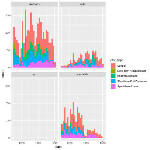
krats <- krats %>% mutate(date = lubridate::ymd(paste(year,month,day,sep='-')))

ggplot(krats, aes(date, fill=plot_type)) +
geom_histogram() +
facet_wrap(~species)
OUTPUT
`stat_bin()` using `bins = 30`. Pick better value with `binwidth`.
This looks much better, and is easier to see the trends over time as well. Note our x axis still shows bins with year labelings, but the continuous spread of our data over these bins shows that dates are treated more continuously and fall more continuously within histogram bins.
Callout
One aspect we can see with this exercise above is that by setting up a reproducible example, we can isolate the problem with data rather than simply asking a proximal problem (i.e. ‘how can i change my plot to look like so’). This allows helpers and you to directly improve your code, but also allows the community to help in identifying the problem. You don’t always need to understand what exact lines of code or function calls are going wrong in order to get help!
Summary
In general, we need to isolate the specific areas of code causing the bug or problem. There is no general rule of thumb as to how large this needs to be, but in general, think about what we would want to include in a reprex. Any early lines which we know run correctly and as intended may not need to be included, and we should seek to isolate the problem area as much as we can to make it understandable to others.
Let’s add to our list of steps for identifying the problem:
Identify the problem area – add print statements immediately upstream or downstream of problem areas, step into functions, and see whether any intermediate output can be further isolated.
Read each part of the error or warning message (if applicable), to see if we can immediately interpret and act on any.
Pulling up the R Documentation for any function calls causing the error (which may be specific to a package, such as with ggplot).
Reading through the documentation’s Description, Usage, Arguments, Details and Examples entries for greater insight into our error.
Copying and pasting the error message into a search engine for more interpretable explanations.
And, when all else fails, preparing our code into a reproducible example for expert help.
Whereas before we had a list of steps for addressing spot problems arising in one or two lines, we can now organize identifying the problem into a more organizational workflow. Any step in the above that helps us identify the specific areas or aspects of our code that are failing in particular, we can zoom in on and restart the checklist. We can stop as soon as we don’t understand anymore how our code fails, at which point we can excise that area for further help.
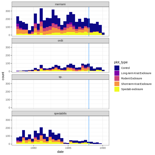
Finally, let’s make our plot publication-ready by changing some aesthetics. Let’s also add a vertical line to show when the study design changed on the exclosures.
R
krats <- rodents %>% filter(genus == "Dipodomys") #kangaroo rat genus
dim(krats)
OUTPUT
[1] 9573 13R
krats <- krats %>% mutate(date = lubridate::ymd(paste(year,month,day,sep='-')))


krats %>%
  ggplot(aes(x = date, fill = plot_type)) +
  geom_histogram()+
  facet_wrap(~species, ncol = 1)+
  theme_bw()+
  scale_fill_viridis_d(option = "plasma")+
  geom_vline(aes(xintercept = lubridate::ymd("1988-01-01")), col = "dodgerblue")
OUTPUT
`stat_bin()` using `bins = 30`. Pick better value with `binwidth`.
It looks like the study change helped to reduce merriami sightings in the Rodent and Short-term Krat exclosures.
