Completely Randomized Design with More than One Treatment Factor
Last updated on 2026-07-16 | Edit this page
Overview
Questions
- How is a CRD with more than one treatment factor designed and analyzed?
Objectives
- .
- .
When experiments are structured with two or more factors, these factors can be qualitative or quantitative. With two or more factors we face the same design issues. Which factors to choose? Which levels for each factor? A full factorial experiment includes all levels of all factors, which can become unwieldy when there are multiple levels for each factor. One option to manage an unwieldy design is to use only a fraction of the factor levels in a fractional factorial design. In this lesson we consider a full factorial design containing all levels of all factors.
A study aims to determine how dosage of a new antidiabetic drug and duration of daily exercise affect blood glucose levels in diabetic mice. The study has two quantitative factors with three levels each.
Drug dosage represents the amount of the antidiabetic drug administered daily. The levels for this factor are in mg per kg body weight. Control mice receive no drug. The second factor, exercise duration, represents the number of minutes the mice run on a running wheel each day. Control mice do not have a running wheel to run on. A full factorial design is used, with each combination of drug dosage and exercise duration applied to a group of mice. For example, one group receives 10 mg/kg of the drug and exercises 30 minutes per day, another group receives 10 mg/kg and exercises 60 minutes per day, and so on.
There are 3 levels for each factor, leading to 9 treatment combinations (3 drug doses × 3 exercise durations). Each combination is replicated with a group of 5 mice, making the design balanced and allowing analysis of interactions. Fasting blood glucose level (mg/dL) was measured at the start and after 4 weeks of treatment. Load the data.
R
drugExercise <- read_csv("data/drugExercise.csv")
drugExercise$DrugDose <- as_factor(drugExercise$DrugDose)
drugExercise$Exercise <- as_factor(drugExercise$Exercise)
head(drugExercise)
OUTPUT
# A tibble: 6 × 5
  DrugDose Exercise Baseline  Delta  Post
  <fct>    <fct>       <dbl>  <dbl> <dbl>
1 0        0            228.  0.449  228.
2 0        0            274. -0.977  273.
3 0        0            236.  0.190  236.
4 0        0            236.  0.731  237.
5 0        0            220  -0.493  220.
6 10       0            246. -5.04   241.
Summarize by mean change in glucose levels (Delta) and
standard deviation.
R
meansSD <- drugExercise %>%
  group_by(Exercise, DrugDose) %>%
  summarise(meanChange = round(mean(Delta), 3),
            stDev = sd(Delta))
meansSD
OUTPUT
# A tibble: 9 × 4
# Groups:   Exercise [3]
  Exercise DrugDose meanChange stDev
  <fct>    <fct>         <dbl> <dbl>
1 0        0            -0.02  0.702
2 0        10           -4.75  1.13
3 0        20           -9.99  0.824
4 30       0            -0.542 0.339
5 30       10           -2.65  1.57
6 30       20           -5.40  0.305
7 60       0            -2.79  0.652
8 60       10           -1.47  0.866
9 60       20           -0.334 0.905
The table shows that the drug alone lowered glucose in the mice in the 0 min/day exercise group. Increasing drug dose also lowered glucose in the 30 min/day exercise group. The 60 min/day exercise group showed the opposite effect. As drug dose increased, average change in glucose diminished.
Boxplots show that exercise alone appears to lower glucose in the mice that were not given the drug. The greatest glucose changes are with a drug dose of 20 mg/kg for 2 of the 3 exercise groups - 0 and 30 minutes of exercise per day. At 60 minutes of exercise a day combined with 20 mg/kg drug dose, change in glucose levels are near zero and don’t seem to have much effect.
R
ggplot(drugExercise, aes(x = DrugDose, y = Delta, fill = Exercise)) +
  geom_boxplot() +
  labs(title = "Change in Glucose by Drug and Exercise",
       y = "Δ Glucose (mg/dL)", x = "Drug Dosage (mg/kg)")
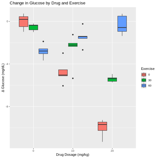
This pattern is repeated for the 10 mg/kg drug dose, where less exercise leads to greater change in glucose levels and more exercise leads to smaller changes. However, each boxplot shows outliers as dots extending above and below the boxes. This makes it difficult to determine if there really is a difference in glucose levels since there is so much overlap between the boxplots and their outliers. In fact, the spread of the data (standard deviation) at 10 mg/kg drug dose are among the largest values in the entire data set. With only 5 mice per group, it is difficult to obtain enough precision to capture the true value of mean glucose change.
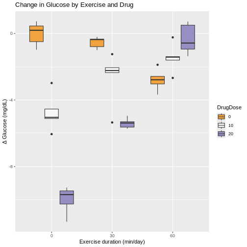
Boxplots with exercise on the x-axis show similar patterns for combinations of exercise and drug dose. Greater variability for some exercise groups is apparent. The 0 min/day exercise group has the greatest within-group variability across all drug doses. The 60 min/day exercise group has the least within-group variability across all drug doses.
R
ggplot(drugExercise, aes(x = Exercise, y = Delta, fill = DrugDose)) +
  geom_boxplot() +
  labs(title = "Change in Glucose by Exercise and Drug",
       y = "Δ Glucose (mg/dL)", x = "Exercise duration (min/day)") +
  scale_fill_brewer(palette = "PuOr") # use a different color palette
Interaction between factors
We could analyze these data as if it were simply a completely randomized design with 9 treatments (3 drug doses and 3 exercise durations). The ANOVA would have 8 degrees of freedom for treatments and the F-test would tell us whether the variation among average changes in glucose levels for the 9 treatments was real or random. However, the factorial treatment structure lets us separate out the variability in glucose level changes among drug doses averaged over exercise durations. The ANOVA table would provide a sum of squares based on 2 degrees of freedom for the difference between the 3 treatment means (\(\bar{y}_i\)) and the pooled (overall) mean (\(\bar{y}\)).
Sum of squares for 9 treatments \(= n\sum(\bar{y}_i - \bar{y})^2\).
The sum of squares would capture the variability among the 3 drug dose levels. The variation among the 3 exercise levels would be captured similarly, with 2 degrees of freedom. That leaves 8 - 4 = 4 degrees of freedom left over. What variability do these remaining 4 degrees of freedom contain? The answer is interaction - the interaction between drug doses and exercise durations.
| source of variation | Df | Sum Sq | Mean Sq=Sum Sq/Df | F value | prob(>F) |
|---|---|---|---|---|---|
| treatment 1 | \(k_1 - 1\) | Sum Sq | Mean Sq=Sum Sq/Df | F value | prob(>F) |
| treatment 2 | \(k_2 - 1\) | Sum Sq | Mean Sq=Sum Sq/Df | F value | prob(>F) |
| interaction | \((k_1 - 1) * (k_2 - 1)\) | Sum Sq | Mean Sq=Sum Sq/Df | F value | prob(>F) |
| error | \(k_1 * k_2 * (n - 1)\) | Sum Sq | Mean Sq=Sum Sq/Df | F value | prob(>F) |
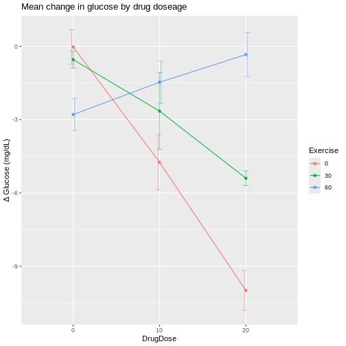
We can visualize interactions for all combinations of drug dose and exercise duration with an interaction plot that shows mean change in glucose levels on the y-axis.
R
ggplot(meansSD, aes(x=DrugDose, y=meanChange, group=Exercise, color=Exercise)) +
    geom_line() +
    geom_point() +
    geom_errorbar(aes(ymin=meanChange-stDev, ymax=meanChange+stDev), width=.2,
                  position=position_dodge(0.05), alpha=.5) +
  labs(y = "Δ Glucose (mg/dL)",
       title = "Mean change in glucose by drug doseage")
R
ggplot(meansSD, aes(x=Exercise, y=meanChange, group=DrugDose, color=DrugDose)) +
    geom_line() +
    geom_point() +
    geom_errorbar(aes(ymin=meanChange-stDev, ymax=meanChange+stDev), width=.2,
                  position=position_dodge(0.05), alpha=.5) +
  labs(y = "Δ Glucose (mg/dL)",
       title = "Mean change in glucose by exercise")
The interaction plots shows wide variation in mean glucose changes at a drug dose of 20 mg/kg, and also at 0 min/day exercise. The vertical bars extending above and below each mean value are the standard deviations for that group. Notice that the bars for the 10 mg/kg drug dose group are the longest, indicating higher variability that we also saw in the boxplots.
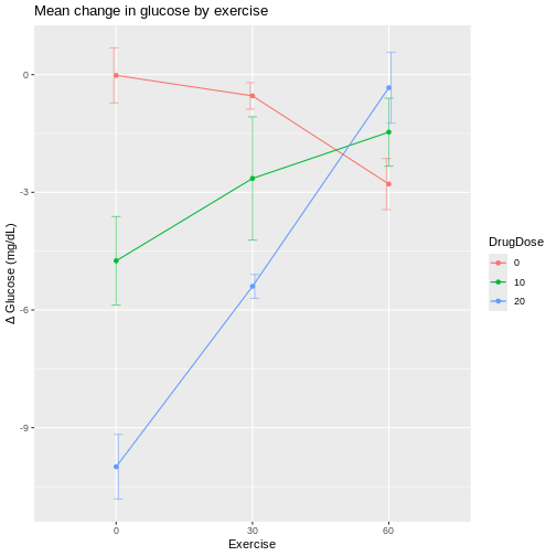
If we plot exercise on the x-axis, the same patterns show up differently.
R
ggplot(meansSD, aes(x=Exercise, y=meanChange, group=DrugDose, color=DrugDose)) +
    geom_line() +
    geom_point() +
    geom_errorbar(aes(ymin=meanChange-stDev, ymax=meanChange+stDev), width=.2,
                  position=position_dodge(0.05), alpha=.5) +
  labs(y = "Δ Glucose (mg/dL)",
       title = "Mean change in glucose by exercise")

At 60 min/day exercise, there is considerable overlap between the standard deviation bars in the three drug dosage groups. There is not a clear distinction indicating that the drug has an effect, although the 0 drug dosage group does appear to benefit from more exercise.
If lines were parallel we could assume no interaction between drug and exercise. Since they are not parallel we should assume interaction between exercise and drug dose. The F-test from an ANOVA will tell us whether this apparent interaction is real or random, specifically whether it is more pronounced than would be expected due to random variation.
R
# DrugDose*Exercise is the interaction
# main effects (DrugDose and Exercise separately) are included
anova(lm(Delta ~ DrugDose*Exercise,
         data = drugExercise))
OUTPUT
Analysis of Variance Table

Response: Delta
                  Df  Sum Sq Mean Sq F value    Pr(>F)
DrugDose           2 128.142  64.071  81.048 4.674e-14 ***
Exercise           2  87.515  43.757  55.352 1.041e-11 ***
DrugDose:Exercise  4 195.265  48.816  61.752 1.271e-15 ***
Residuals         36  28.459   0.791
---
Signif. codes:  0 '***' 0.001 '**' 0.01 '*' 0.05 '.' 0.1 ' ' 1
We can read the ANOVA table from the bottom up, starting with the
interaction (DrugDose:Exercise). The F value
for the interaction is 61.75 on 4 and 36 degrees of freedom for the
interaction and error (Residuals) respectively. The p-value
(Pr(>F)) is very low and as such the interaction between
exercise and drug dose is significant, backing up what we see in the
interaction plots.
If we move up a row in the table to Exercise, the F test
compares the mean changes across drug dose groups. The
F value for exercise is 55.35 on 2 and 36 degrees of
freedom for exercise and residuals respectively. The p-value is very low
and so exercise is significant. Finally, we move up to the row
containing DrugDose to find an F value of 81.05 and a very
low p-value again. Drug dose averaged over exercise is significant.
The partitioning of treatments sums of squares into main effect (average) and interaction sums of squares is a result of the crossed factorial structure (orthogonality) of the two factors. The complete combinations of these two factors provides clean partitioning between main effects and interactions. This is not to say that designs that don’t have full combinations of factors can’t be analyzed to estimate main effects and interactions. They can be analyzed with generalized linear models.
The development of efficient and informative multifactorial designs that cleanly separate main effects from interactions is one of the most important contributions of statistical experimental design.
- Completely randomized designs can be structured with two or more factors.
- Random assignment of treatments to experimental units in a single homogeneous group is the same.
- Factorial structure of the experiment requires different analyses, primarily ANOVA.