Overview
Teaching: 30 min
Exercises: 0 minQuestions
How to connect to database with python?
What is in the database?
What are common datatypes in SQL?
Objectives
Load the database
Learn how to run query in python
Learn what is in the database
Define SQLite data types.
Setup
Note: this should have been done by participants before the start of the workshop.
See Setup for instructions on how to download the data, and also how to install and open SQLite Manager.
Import
Before we get started with writing our own queries, we’ll load the data into the database. We’ll need the following file:
soda.db
Dataset Description
The data we will be using is soda sells data. It contains invoice information about soda purchase from soda makers (vendors) by retail stores. The data was originated from a real dataset. We have modified the dataset for this workshop. For example, soda names are completely fictitious, and price was also normalized.
- In an jupyter notebook cell, put in the following code to import sqlite3 and pandas modules:
import sqlite3 as sql import pandas as pdsqlite3will be included within a standard Python installation.pandasis not part of the Python Standard Library, but will normally be bundled with Anaconda. - in the next cell, create a connection to the database called conn
conn = sql.connect('soda.db') - In the next cell, write your query as string called “q” (you can call it whatever you want). The following example is to select everything in a table called item_info:
q = ''' SELECT * FROM item_info; ''' - The pandas package in Python has a built in function to read sql.
The following code will execute the query and assign the result to a DataFrame variable called “df”, and show the result (use .head(10) to show first 10 result, you can remove that part to show the full result):
df = pd.read_sql(q, conn) df.head(10) # df or print(df) can show the whole result - To run a different query, you can just change the query string between
''' '''and run the code above again.
For example,q = ''' SELECT * FROM invoice_info; ''' df = pd.read_sql(q, conn) df.head(10)You just ran your first SQL query! Now, lets see what’s in the database
Database Organization
- List all the tables in the soda database
q = ''' SELECT * FROM sqlite_master; ''' df = pd.read_sql(q, conn) df - List the fields/columns in each table
print(df['sql'][0])
print(df['sql'][1])
print(df['sql'][3])
print(df['sql'][4])
print(df['sql'][5])
print(df['sql'][6])
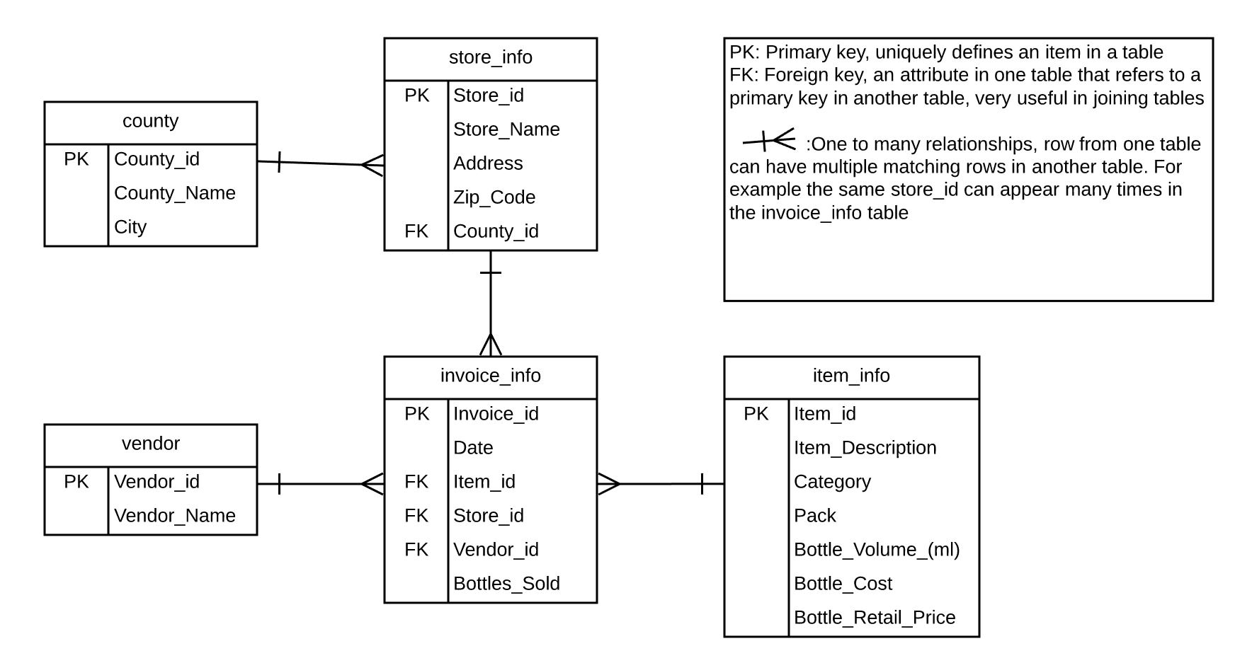
To have a better understanding of Primary keys and Foreign keys discussed in previous session, lets look at the tables and their relationships:
Data types
Here are all the attributes in the database:
| Attributes | Data Type | Description | Table(s) |
|---|---|---|---|
| County_id | INTEGER | Unique id for each county | county, store_info |
| County_Name | TEXT | Name of county | county |
| City_Name | TEXT | Name of the city that the county is in | county |
| Category | VARCHAR(20) | Category of soda | item_info |
| Vendor_id | INTEGER | Unique id for each vendor | vendor, invoice_info |
| Vendor_Name | TEXT | Name of the vendor | vendor |
| Store_id | INTEGER | Unique id for each store | store_info, invoice_info |
| Store_Name | TEXT | Name of the store | store_indo |
| Address | TEXT | Address of the store | store_info |
| Zip_Code | INTEGER | Zip code of the store | store_info |
| Item_id | INTEGER | Unique id for each item (soda) | item_info, invoice_id |
| Item_Description | TEXT | Name of the item (soda) | item_info |
| Pack | INTEGER | Number of bottles that the soda usually sells for | item_info |
| Bottle_Volume_ml | DOUBLE | Volume of the soda in ml | item_info |
| Bottle_Cost | DOUBLE | Cost of one bottle | item_info |
| Bottle_Retail_Price | DOUBLE | Retile price for one bottle | item_info |
| Invoice_id | VARCHAR(20) | Unique id for each invoice | invoice_info |
| Date | TEXT | Date of the invoice | invoice_info |
| Bottle_Sold | INTEGER | Number of bottle sold in the invoice | invoice_info |
Here are few common SQL datatypes (just FYI):
- Note that SQLite does not have a separate storage class for storing dates and/or times, but SQLite is capable of storing dates and times as TEXT, REAL or INTEGER values. In the database we used today, the date attribute is stored as text in “YYYY-MM-DD” format. We will talk about this later.
| Data type | Description |
|---|---|
| CHARACTER(n) | Character string. Fixed-length n |
| VARCHAR(n) or CHARACTER VARYING(n) | Character string. Variable length. Maximum length n |
| BINARY(n) | Binary string. Fixed-length n |
| BOOLEAN | Stores TRUE or FALSE values |
| VARBINARY(n) or BINARY VARYING(n) | Binary string. Variable length. Maximum length n |
| INTEGER(p) | Integer numerical (no decimal). |
| SMALLINT | Integer numerical (no decimal). |
| INTEGER | Integer numerical (no decimal). |
| BIGINT | Integer numerical (no decimal). |
| DECIMAL(p,s) | Exact numerical, precision p, scale s. |
| NUMERIC(p,s) | Exact numerical, precision p, scale s. (Same as DECIMAL) |
| FLOAT(p) | Approximate numerical, mantissa precision p. A floating number in base 10 exponential notation. |
| REAL | Approximate numerical |
| FLOAT | Approximate numerical |
| DOUBLE | Approximate numerical |
| DATE* | Stores year, month, and day values |
| TIME* | Stores hour, minute, and second values |
| TIMESTAMP* | Stores year, month, day, hour, minute, and second values |
| INTERVAL | Composed of a number of integer fields, representing a period of time, depending on the type of interval |
| ARRAY | A set-length and ordered collection of elements |
| MULTISET | A variable-length and unordered collection of elements |
| XML | Stores XML data |
SQL Data Type Quick Reference
Different databases offer different choices for the data type definition.
The following table shows some of the common names of data types between the various database platforms:
| Data type | Access | SQLServer | Oracle | MySQL | PostgreSQL |
|---|---|---|---|---|---|
| boolean | Yes/No | Bit | Byte | N/A | Boolean |
| integer | Number (integer) | Int | Number | Int / Integer | Int / Integer |
| float | Number (single) | Float / Real | Number | Float | Numeric |
| currency | Currency | Money | N/A | N/A | Money |
| string (fixed) | N/A | Char | Char | Char | Char |
| string (variable) | Text (<256) / Memo (65k+) | Varchar | Varchar2 | Varchar | Varchar |
| binary object OLE Object Memo Binary (fixed up to 8K) | Varbinary (<8K) | Image (<2GB) Long | Raw Blob | Text Binary | Varbinary |
Key Points
We can import sqlite3 to work with relational database in python
Primary key uniquely identifies each rows in a table. A foreign key in one table refers to a primary key in another table.
Common data types in SQL are are integer, varchar, char, text, double, etc.