Working with MRI
Last updated on 2024-12-29 | Edit this page
Estimated time: 90 minutes
Overview
Questions
- What kinds of MRI are there?
- How are MRI data represented digitally?
- How should I organize and structure files for neuroimaging MRI data?
Objectives
- Mention common kinds of MRI imaging used in research
- Show the most common file formats for MRI
- Introduce MRI coordinate systems
- Load an MRI scan into Python and explain how the data is stored
- View and manipulate image data
- Explain what BIDS is
- Explain advantages of working with Nifti and BIDS
- Show a method to convert from DICOM to BIDS/NIfTI
Introduction
When some programmers open their IDE, they type pwd
because this command allows you to see what directory you are in, and
then often they type git branch to see which branch they
are on. When many clinicians open an MRI they look at the anatomy, but
also figure out which sequence and type of MRI they are looking at. We
all need to begin with a vague idea of where in the world we are and
which direction we are facing, so to speak. As a digital researcher
orienting yourself in terms of MRIs and related computation is
important. In terms of computation MRIs, particularly neuro MRIs, have
some quirks that make it worthwhile to think of them as a separate part
of the universe than other medical imaging. Three critical differences
between MRIs and other medical imaging are image orientation in terms of
display conventions, typical file types and typical packages used for
processing. In this lesson we will cover these three issues.
As a researcher in general we recommend familiarizing yourself with
the various possible sequences of MRI. Some sequences are much more
suited to answer certain questions than others. Generally we could
divide MR techniques into structural e.g. T1, T2 and so on, functional,
diffusion, perfusion, angiographic techniques and spectroscopy. The
sequences you work with determining the shape of files to expect. As an
example of what you would expect for structural imaging a 3-D array is
the norm, but for diffusion imaging you have a 4D tensor plus .bval and
.bvec files.
If you work directly with a radiology department you will usually get
DICOM files that contain whatever sequences were done. However if you
obtain images from elsewhere they may come in other formats.
File formats
From the MRI scanner, MRI images are initially collected and put in the DICOM format but can be converted to other formats to make working with the data easier. Some file formats can be converted to others, for example NiFTIs or Analyze files can be converted to MINC, but not conversions can not be made from all file formats in all directions.
Common MRI File Formats
To understand common file formats please review the table on neuroimaging file formats here. To get even more information than that table we have included links to documentation websites:
NIfTI is one of the most ubiquitous file formats for storing
neuroimaging data. We can convert DICOM data to NIfTI using dcm2niix software. Many
people prefer working with dcm2bids to configure long bash
commands needed for dcm2niix.
For example if you just want to write bash using dcm2niix or dcm2bids to place a convert a hypothetical DICOM file (in a directory /hypothetical) into a hypothetical directory called /converted on your machine you can do it in the following way:
dcm2biids_helper -d /hypothetical -o /converted
One of the advantages of working with dcm2niix, whether
you work with it directly or with a tool like dcm2bids is
that it can be used to create Brain Imaging Data Structure (BIDS) files,
since it outputs a NIfTI and a JSON with metadata ready to fit into the
BIDS standard. BIDS is a
widely adopted standard of how data from neuroimaging research can be
organized. The organization of data and files is crucial for seamless
collaboration across research groups and even between individual
researchers. Some pipelines assume your data is organized in BIDS
structure, and these are sometimes called BIDS Apps.
Some of the more popular examples are:
fmriprepfreesurfermicapipeSPMMRtrix3_connectome
We recommend the BIDS starter-kit website for learning the basics of this standard. Working with BIDS or and much of the array of tools available for brain MRIs is often facilitated by some familiarity with writing command line. This could present bit of a problem in terms of scientific reproducibility. One option is to leave bash scripts and good documentation in a repository. Another is to use a pythonic interface to such command line tools. One possibility for this will be discussed in the next section.
Libraries
If you look at python code for research on medical imaging of most of the body, a few libraries, such as SITK, will pop up again and again. The story with MRIs of the brain is entirely different. Most researchers will use libraries like nibabel and related libraries. These libraries are made to read, write, and manipulate neuroimaging file formats efficiently. There is lots of code developed in them for the specific tasks related to brain MRIs. They also tend to integrate better with existing pipelines for brain MRI. nipype is a popular tool which attempts to allow users to harness popular existing pipelines. If you are trying to compare outputs with an existing study, it is worth considering using the same pipeline and software version of the pipeline. Then you know differences between your outcomes are not artifacts of the softwares.
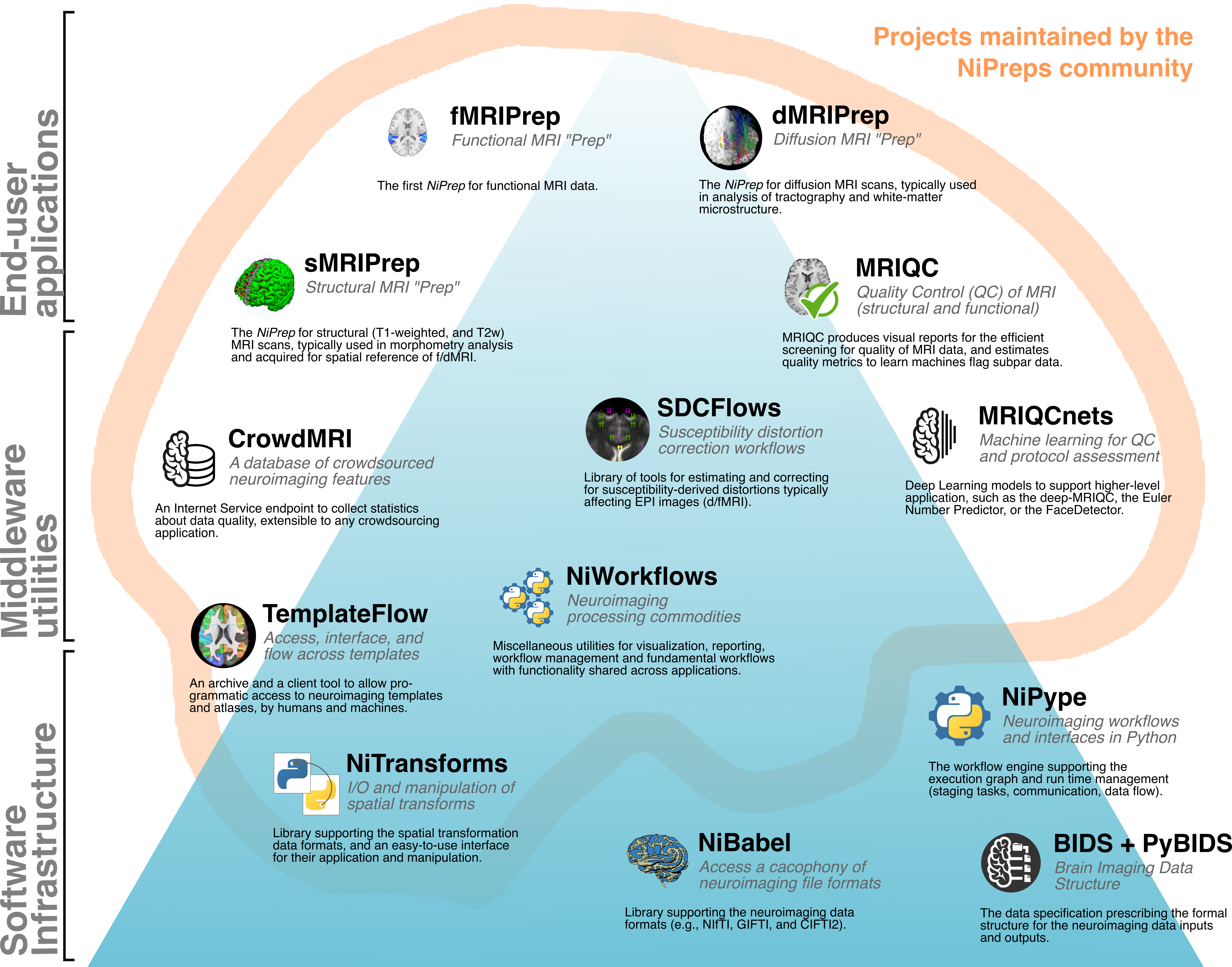
Sourced from https://www.nipreps.org/
Nipreps and Beyond:
- There are many, many packages for medical image analysis
- There are known pre-built pipelines with possibilities in python
- Your pipeline will probably begin with cleaning and preparing data
- You can mix and match parts of pipelines with NiPype
While you may harness sophisticated tools like Freesurfer or FSL to do complex tasks like segmentation and registration in ways that match existing research, you should not avoid checking your data by hand. At some point you should open images and examine them both in terms of the imaging (which could be done with a pre-built viewer) and the computational aspects like metadata and shape. For these mundane tasks we recommend nibabel.
Next, we’ll cover some details on working with NIfTI files with Nibabel.
Reading NIfTI Images
NiBabel is a Python package for reading and writing neuroimaging data. To learn more about how NiBabel handles NIfTIs, refer to the NiBabel documentation on working with NIfTIs, which this episode heavily references. This part of the lesson is also similar to an existing lessons from The Carpentries Incubator; namely: Introduction to Working with MRI Data in Python. This is because in terms of reading and loading data and accessing the image, there are limited possibilities.
First, use the load() function to create a
NiBabel image object from a NIfTI file.
When loading a NIfTI file with NiBabel, you get a
specialized data object that includes all the information stored in the
file. Each piece of information is referred to as an
attribute in Python’s terminology. To view all these
attributes, simply type t2_img. followed by Tab.
We will focus on discussing mainly two attributes (header
and affine) and one method (get_fdata).
1. Headers
The header contains metadata about the image, including image dimensions, data type, and more.
OUTPUT
<class 'nibabel.nifti1.Nifti1Header'> object, endian='<'
sizeof_hdr      : 348
data_type       : b''
db_name         : b''
extents         : 0
session_error   : 0
regular         : b''
dim_info        : 0
dim             : [  3 432 432  30   1   1   1   1]
intent_p1       : 0.0
intent_p2       : 0.0
intent_p3       : 0.0
intent_code     : none
datatype        : int16
bitpix          : 16
slice_start     : 0
pixdim          : [1.        0.9259259 0.9259259 5.7360578 0.        0.        0.
 0.       ]
vox_offset      : 0.0
scl_slope       : nan
scl_inter       : nan
slice_end       : 29
slice_code      : unknown
xyzt_units      : 2
cal_max         : 0.0
cal_min         : 0.0
slice_duration  : 0.0
toffset         : 0.0
glmax           : 0
glmin           : 0
descrip         : b'Philips Healthcare Ingenia 5.4.1 '
aux_file        : b''
qform_code      : scanner
sform_code      : unknown
quatern_b       : 0.008265011
quatern_c       : 0.7070585
quatern_d       : -0.7070585
qoffset_x       : 180.81993
qoffset_y       : 21.169691
qoffset_z       : 384.01007
srow_x          : [1. 0. 0. 0.]
srow_y          : [0. 1. 0. 0.]
srow_z          : [0. 0. 1. 0.]
intent_name     : b''
magic           : b'n+1'
t2_hdr is a Python dictionary, i.e. a
container that hold pairs of objects - keys and values. Let’s take a
look at all of the keys.
Similar to t2_img, in which attributes can be accessed
by typing t2_img. followed by Tab, you can do
the same with t2_hdr.
In particular, we’ll be using a method belonging to
t2_hdr that will allow you to view the keys associated with
it.
OUTPUT
['sizeof_hdr',
 'data_type',
 'db_name',
 'extents',
 'session_error',
 'regular',
 'dim_info',
 'dim',
 'intent_p1',
 'intent_p2',
 'intent_p3',
 'intent_code',
 'datatype',
 'bitpix',
 'slice_start',
 'pixdim',
 'vox_offset',
 'scl_slope',
 'scl_inter',
 'slice_end',
 'slice_code',
 'xyzt_units',
 'cal_max',
 'cal_min',
 'slice_duration',
 'toffset',
 'glmax',
 'glmin',
 'descrip',
 'aux_file',
 'qform_code',
 'sform_code',
 'quatern_b',
 'quatern_c',
 'quatern_d',
 'qoffset_x',
 'qoffset_y',
 'qoffset_z',
 'srow_x',
 'srow_y',
 'srow_z',
 'intent_name',
 'magic']
Notice that methods require you to include () at the end of them when you call them whereas attributes do not. The key difference between a method and an attribute is:
- Attributes are variables belonging to an object and containing information about their properties or characteristics
- Methods are functions that belong to an object and operate on its
attributes. They differ from regular functions by implicitly receiving
the object (
self) as their first argument.
When you type in t2_img. followed by Tab, you
may see that attributes are highlighted in orange and methods
highlighted in blue.
The output above is a list of keys you can use to
access values of t2_hdr. We can access the
value stored by a given key by typing:
Challenge: Extract Values from the NIfTI Header
Extract the ‘pixdim’ field from the NiFTI header of the loaded image.
2. Data
As you’ve seen above, the header contains useful information that
gives us information about the properties (metadata) associated with the
MR data we’ve loaded in. Now we’ll move in to loading the actual
image data itself. We can achieve this by using the method
called t2_img.get_fdata():
OUTPUT
array([[[0., 0., 0., ..., 0., 0., 0.],
        [0., 0., 0., ..., 0., 0., 0.],
        [0., 0., 0., ..., 0., 0., 0.],
        ...,
        [0., 0., 0., ..., 0., 0., 0.],
        [0., 0., 0., ..., 0., 0., 0.],
        [0., 0., 0., ..., 0., 0., 0.]],

       [[0., 0., 0., ..., 0., 0., 0.],
        [0., 0., 0., ..., 0., 0., 0.],
        [0., 0., 0., ..., 0., 0., 0.],
        ...,
        [0., 0., 0., ..., 0., 0., 0.],
        [0., 0., 0., ..., 0., 0., 0.],
        [0., 0., 0., ..., 0., 0., 0.]],

       ...,

       [[0., 0., 0., ..., 0., 0., 0.],
        [0., 0., 0., ..., 0., 0., 0.],
        [0., 0., 0., ..., 0., 0., 0.],
        ...,
        [0., 0., 0., ..., 0., 0., 0.],
        [0., 0., 0., ..., 0., 0., 0.],
        [0., 0., 0., ..., 0., 0., 0.]]])
The initial observation you might make is the prevalence of zeros in the image. This abundance of zeros might prompt concerns about the presence of any discernible content in the picture. However, when working with radiological images, it’s important to keep in mind that these images frequently contain areas of air surrounding the objects of interest, which appear as black space.
What type of data is this exactly in a computational sense? We can
determine this by calling the type() function on
t2_data:
OUTPUT
numpy.ndarrayThe data is stored as a multidimensional array,
which can also be accessed through the file’s dataobj
property:
OUTPUT
<nibabel.arrayproxy.ArrayProxy at 0x20c63b5a4a0>As you might guess there are differences in how your computer handles something made with dataobj and an actual array. These differences effect memory and processing speed. These are not trivial issues if you deal with a very large dataset of MRIs. You can save time and memory by being conscious about what is cached and using the dataobj property when dealing with slices of the array as detailed here
Challenge: Meaning of Attributes of the Array
How can we see the number of dimensions in the t2_data
array? Once again, all of the attributes of the array can be seen by
typing t2_data. followed by Tab. What is the
shape of the image? Can you make a guess about then size of a voxel
based on the numbers you have here? Why or why not?
OUTPUT
3t2_data contains 3 dimensions. You can think of the data
as a 3D version of a picture (more accurately, a volume).
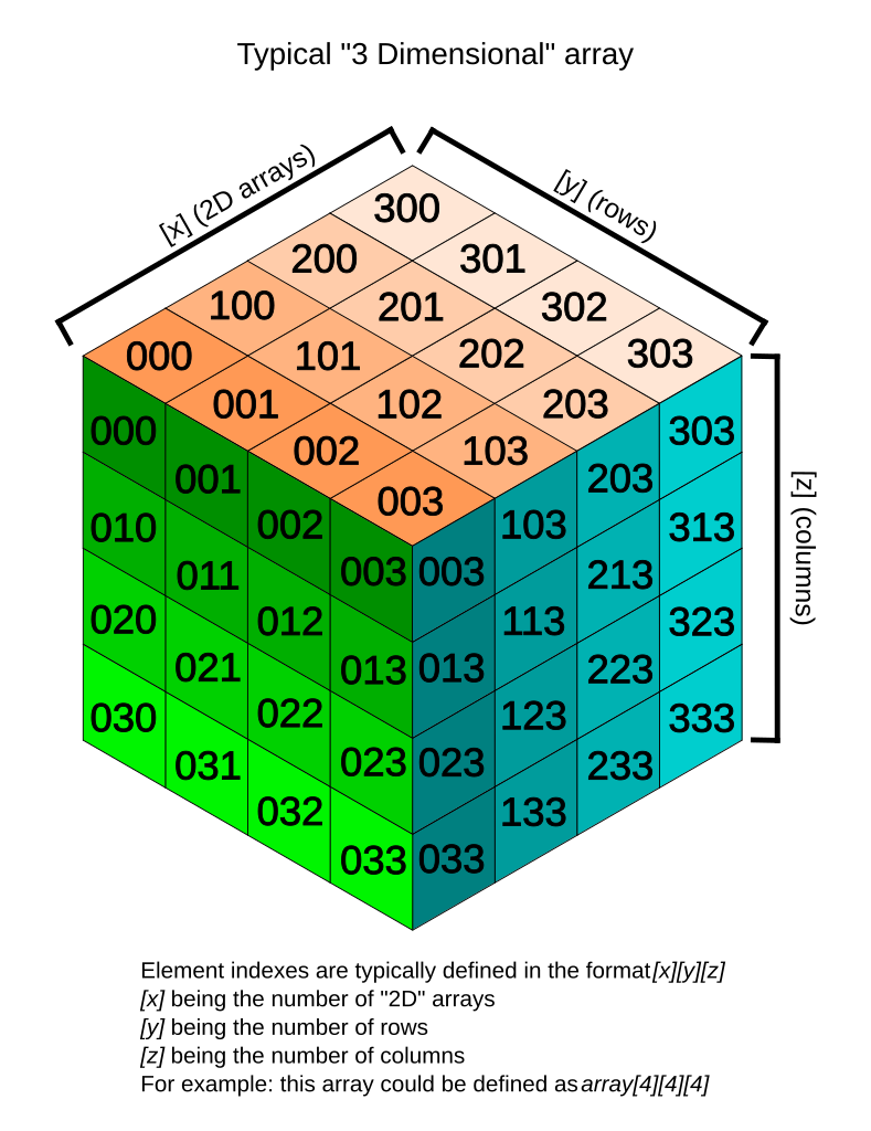
Image by Tropwine, sourced from Wikimedia Commons (2024).https://commons.m.wikimedia.org/wiki/File:3D_array_diagram.svg; Creative Commons Attribution 4.0 International License
Remember typical 2D pictures are made out of pixels, but a 3D MR image is made up of 3D cubes called voxels.
Sourced with minor modification from Ahmed, M., Garzanich, M., Melaragno, L.E. et al. Exploring CT pixel and voxel size effect on anatomic modeling in mandibular reconstruction. 3D Print Med 10, 21 (2024). https://doi.org/10.1186/s41205-024-00223-0; Creative Commons Attribution 4.0 International License
With this in mind we examine the shape:
OUTPUT
(432, 432, 30)The three numbers given here represent the number of values along a respective dimension (x,y,z). This image was scanned in 30 slices, each with a resolution of 432 x 432 voxels. If each voxel were 1 millimeter, then our image would represent something 3cm tall (so to speak), and this seems unlikely. However, object here is not human, and could be in theory be scanned on a special MRI machine of any size. We can not make a guess from the data we printed here alone about the size of a voxel. We will learn one method to do this later in the episode.
Let’s see the type of data inside of the array.
OUTPUT
dtype('float64')This tells us that each element in the array (or voxel) is a
floating-point number.
The data type of an image controls the range of possible intensities. As
the number of possible values increases, the amount of space the image
takes up in memory also increases.
OUTPUT
0.0
630641.0785522461
For our data, the range of intensity values goes from 0 (black) to more positive digits (whiter).
To examine the value of a specific voxel, you can access it using its
indices. For example, if you have a 3D array data, you can
retrieve the value of a voxel at coordinates (x, y, z) with the
following syntax:
This will give you the value stored at the voxel located at the
specified index (x, y, z). Make sure that the indices are
within the bounds of the array dimensions.
To inspect the value of a voxel at coordinates (9, 19, 2), you can use the following code:
OUTPUT
0.This command retrieves and prints the intensity value at the specified voxel. The output represents the signal intensity at that particular location.
Next, we will explore how to extract and visualize larger regions of interest, such as slices or arrays of voxels, for more comprehensive analysis.
Working with Image Data
When we think and speak about about “slicing” colloqiually, we often think about a 2D slice from our data.
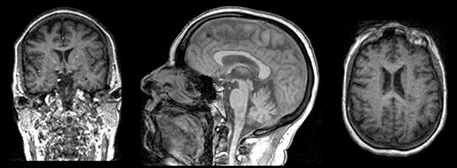
Figure with adaptation from Valdes-Hernandez, P.A., Laffitte Nodarse, C., Peraza, J.A. et al. Toward MR protocol-agnostic, unbiased brain age predicted from clinical-grade MRIs. Sci Rep 13, 19570 (2023). https://doi.org/10.1038/s41598-023-47021-y ; Creative Commons Attribution 4.0 International License
From left to right: coronal, saggital and axial slices of a brain.
Let’s select the 10th slice in the z-axis of our data:
This is similar to the indexing we did before to select a single
voxel. However, instead of providing a value for each axis, the
: indicates that we want to grab all values from
that particular axis.
In the nibabel documentation there are more details on how to use a
slicer attribute of a nibabel array data. Using this
attribute can help to make code more efficient.
Challenge: Slicing MRI Data
Write a python function using nibabel to take an image string, and
coordinates for any slices desired on x, y and z axes; and plot the
image slices. Then use the function to display slices of
t2_data at x = 9, y = 9, and z= 9.
PYTHON
# if in a new notebook re-import
import nibabel as nib
import numpy as np
import matplotlib.pyplot as plt


def slice_image_data(file_path, x, y, z):
    # load the image
    try:
        img = nib.load(file_path)
    except Exception as e:
        print(f"Error loading the image: {e}")
        return

    # get the image array
    data = img.get_fdata()

    # slice the image data
    # and extract a specific slice along each plane
    z_slice = data[:, :, z]  # slice
    y_slice = data[:, y, :]  # slice
    x_slice = data[x, :, :]  # slice
    # make each slice is 2D by explicitly removing unnecessary dimensions
    z_slice = z_slice.squeeze()  # this ensures it's a 2D array
    y_slice = y_slice.squeeze()
    x_slice = x_slice.squeeze()

    print(z_slice.shape)

    # visualize the slices
    plt.figure(figsize=(12, 8))

    # plot the z slice
    plt.subplot(2, 2, 1)
    plt.imshow(z_slice.T, cmap='gray', origin='lower')
    plt.title('Z Slice')
    plt.axis('off')

    # plot the y slice
    plt.subplot(2, 2, 2)
    plt.imshow(y_slice.T, cmap='gray', origin='lower')
    plt.title('Y Slice')
    plt.axis('off')

    # plot the x slice
    plt.subplot(2, 2, 3)
    plt.imshow(x_slice.T, cmap='gray', origin='lower')
    plt.title('X Slice')
    plt.axis('off')

slice_image_data('data/mri//OBJECT_phantom_T2W_TSE_Cor_14_1.nii',9,9,9)
In the above exercise you may note many solutions do not return anything. This is not unusal in Python when we only want a graph or visualization. We really only want an artifact of some functions, however we could return the artifact with more code if needed.
We’ve been slicing and dicing images but we have no idea what they look like in a more global sense. In the next section we’ll show you one way you can visualize it all together.
Visualizing the Data
We previously inspected the signal intensity of the voxel at coordinates (10,20,3).
We could look at the whole image at once by using a viewer. We can even use code to make a viewer.
PYTHON
import numpy as np
import matplotlib.pyplot as plt
import ipywidgets as widget
import nibabel as nib
import importlib


class NiftiSliceViewer:
    """
    A class to examine slices of MRIs, which are in Nifti Format. Similar code appears
    in several open source liberally licensed libraries written by drcandacemakedamoore

    """

    def __init__(self, volume_str, figsize=(10, 10)):
        self.nifti = nib.load(volume_str)
        self.volume = self.nifti.get_fdata()
        self.figsize = figsize
        self.v = [np.min(self.volume), np.max(self.volume)]
        self.widgets = importlib.import_module('ipywidgets')

        self.widgets.interact(self.transpose, view=self.widgets.Dropdown(
            options=['axial', 'saggital', 'coronal'],
            value='axial',
            description='View:',
            disabled=False))

    def transpose(self, view):
        # transpose the image to orient according to the slice plane selection
        orient = {"saggital": [1, 2, 0], "coronal": [2, 0, 1], "axial": [0, 1, 2]}
        self.vol = np.transpose(self.volume, orient[view])
        maxZ = self.vol.shape[2] - 1

        self.widgets.interact(
            self.plot_slice,
            z=self.widgets.IntSlider(
                min=0,
                max=maxZ,
                step=1,
                continuous_update=True,
                description='Image Slice:'
            ),
        )

    def plot_slice(self, z):
        # plot slice for plane which will match the widget intput
        self.fig = plt.figure(figsize=self.figsize)
        plt.imshow(
            self.vol[:, :, z],
            cmap="gray",
            vmin=0,
            vmax=self.v[1],
        )
# now we wil use our class on our image
NiftiSliceViewer('data/mri//OBJECT_phantom_T2W_TSE_Cor_14_1.nii')
Notice our viewer has axial, saggital and coronal slices. These are anatomical terms that allow us to make some assumptions about where things are in space if we assume the patient went into the machine in a certain way. When we look at an abstract image, these terms have little meaning, but let’s take a look at a head.
Challenge: Understanding anatomical terms for brains
Use the internet to read at least two sources on the meaning of the terms axial, coronal and saggital. Write definitions for axial, saggital and coronal in terms of how they slice up the head at the eyes in your own words.
Axial: Slices the head as if slicing across both eyes, such that there is a slice between higher and lower levels Saggital: Slicing between or on the side of the eyes, such that there is a slice between more left and more right Coronal: Slicing both eyes such that there is a slice between front and back levels
This brings us to the final crucial attribute of a NIfTI we will discuss: affine.
3. Affine
The final important piece of metadata associated with an image file is the affine matrix, which indicates the position of the image array data in the reference space. By reference space we usually mean a predefined system mapping to real world space if we are talking about real patient data.
Below is the affine matrix for our data:
OUTPUT
array([[-9.25672975e-01,  2.16410652e-02, -1.74031337e-05,
         1.80819931e+02],
       [ 2.80924864e-06, -3.28338569e-08, -5.73605776e+00,
         2.11696911e+01],
       [-2.16410652e-02, -9.25672975e-01, -2.03403855e-07,
         3.84010071e+02],
       [ 0.00000000e+00,  0.00000000e+00,  0.00000000e+00,
         1.00000000e+00]])
To explain this concept, recall that we referred to coordinates in our data as (x,y,z) coordinates such that:
- x is the first dimension of
t2_data - y is the second dimension of
t2_data - z is the third dimension of
t2_data
Although this tells us how to access our data in terms of voxels in a 3D volume, it doesn’t tell us much about the actual dimensions in our data (centimetres, right or left, up or down, back or front). The affine matrix allows us to translate between voxel coordinates in (x,y,z) and world space coordinates in (left/right, bottom/top, back/front). An important thing to note is that in reality in which order you have:
- Left/right
- Bottom/top
- Back/front
Depends on how you’ve constructed the affine matrix; thankfully there is in depth coverage of the issue the nibabel documentation For most of the the data we’re dealing with we use a RAS coordinate system so it always refers to:
- Right
- Anterior
- Superior
Increasing a coordinate value in the first dimension corresponds to moving to the right of the person being scanned, and so on. In the real world whatever orientation you put something in may make someone unhappy. Luckily you can quickly change arrays around in terms of direction by simply using an already efficient numpy functions. Two functions in numpy that can be generalized to make any orientation of an image are numpy.flip() and numpy.rot90(), however there are other functions which are quite convenient for 2D arrays, as displayed below.
PYTHON
import numpy as np
slices = [z_slice, np.fliplr(z_slice), np.flipud(z_slice)]
fig, axes = plt.subplots(1, len(slices))
for i, slice in enumerate(slices):
    axes[i].imshow(slice, cmap="gray", origin="lower")
OUTPUT
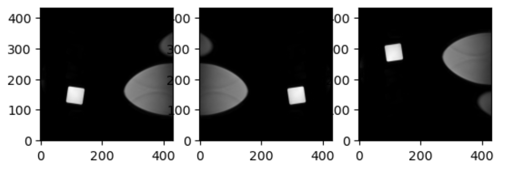
This brings us to a final difference we must account for when we discuss neuro-MRIs: anatomy and visualization conventions.
Display conventions
When we describe imaging of any part of the body except the brain, as professionals we all agree on certain conventions. We rely on anatomical position as the basis of how we orient ourselves, and we expect the patient’s right side to be on the left of our screen, and certain other convensions. In terms of brain MRIs, this is less true; there is a split. The issue is extremely well summarized in the nibabel documentation on radiological versus neurological conventions.
MRI processing in Python
To get a deeper view of MRI processing in Python you can explore lessons from Carpentries Incubators; namely: